 Weihao Chen
 Lumei Su1,2*
 Zhihao Huang
- 1School of Electrical Engineering and Automation, Xiamen University of Technology, Xiamen, China
- 2Xialong Institute of Engineering and Technology, Longyan, China
Rock image classification is a significant part of geological research. Compared with traditional image classification methods, rock image classification methods based on deep learning models have the great advantage in terms of automatic image features extraction. However, the rock classification accuracies of existing deep learning models are unsatisfied due to the weak feature extraction ability of the network model. In this study, a deep residual neural network (ResNet) model with the transfer learning method is proposed to establish the corresponding rock automatic classification model for seven kinds of rock images. ResNet34 introduces the residual structure to make it have an excellent effect in the field of image classification, which extracts high-quality rock image features and avoids information loss. The transfer learning method abstracts the deep features from the shallow features, and better express the rock texture features for classification in the case of fewer rock images. To improve the generalization of the model, a total of 3,82,536 rock images were generated for training via image slicing and data augmentation. The network parameters trained on the Texture Library dataset which contains 47 types of texture images and reflect the characteristics of rocks are used for transfer learning. This pre-trained weight is loaded when training the ResNet34 model with the rock dataset. Then the model parameters are fine-tuned to transfer the model to the rock classification problem. The experimental results show that the accuracy of the model without transfer learning reached 88.1%, while the model using transfer learning achieved an accuracy of 99.1%. Aiming at geological engineering field investigation, this paper studies the embedded deployment application of the rock classification network. The proposed rock classification network model is transplanted to an embedded platform. By designing a rock classification system, the off-line rock classification is realized, which provides a new solution for the rock classification problem in the geological survey. The deep residual neural network and transfer learning method used in this paper can automatically classify rock features without manually extracting. These methods reduce the influence of subjective factors and make the rock classification process more automatic and intelligent.
1 Introduction
Rock classification is the basis for studying geological reservoir characteristics and plays an essential role in vast fields, such as geotechnical engineering, mineralogy, petrology, rock mechanics, and mineral resource prospecting (Karimpouli and Tahmasebi, 2019; Guo et al., 2022; Houshmand et al., 2022). The efficiency of rock classification is closely associated with the efficiency of geological surveys and therefore needs urgent attention. Rocks classification can be accomplished via traditional methods, including remote sensing, electromagnetic field, geochemistry, hand specimen and thin section analysis (Ru and Jiong, 2019). These traditional methods are based on human observation, manual operation and empirical classification. Rock classification using traditional methods mainly extracts useful information features from rock images by professionals through specialized equipment, relying on people’s experience and equipment sensitivity. These methods are often limited by the professionalism of experimental equipment and the theoretical level of researchers, resulting in much time spent, low efficiency and many other problems.
Rock classification using traditional machine learning methods usually need to manually design feature extraction methods and input rock features into the classifier for training, to realize rock classification. Singh et al. (2010) used a multilayer perceptron to extract 27 features from basalt rock slice images and achieved the classification of 140 rock sample slice images. Gonçalves and Leta (2010) proposed a neuro-fuzzy hierarchical classification method based on binary space division for macroscopic rock structure classification, and the final classification accuracy reached 73%. Młynarczuk et al. (2013) used the nearest neighbor algorithm and k-nearest neighbor algorithm to realize the classification of 9 different types of rocks. Sharif et al. (2015) proposed an autonomous rock classification system based on Bayesian image analysis for planetary geological exploration. The rock sample surface was described by 13 Haralick texture parameters and the information was automatically catalogued into a 5-bin data structure, then the Bayesian probability was calculated and the recognition result was output. Patel and Chatterjee (2016) realized the classification of limestone by extracting color, shape and texture features from limestone images and inputting them into a probabilistic neural network. Wang and Sun (2021) proposed a rock classification method using geometric features of rock particles instead of local structural features, which effectively solved the problem of fuzzy boundaries.
With the development of artificial intelligence, machine learning and deep learning are widely used in various image classification problems. Since traditional machine learning need to manually extract rock features from a huge training dataset, the training work is difficult and rather laborious. Using deep learning methods to construct automatic rock classification models has become a new way for rock classification (Fan et al., 2020; Falivene et al., 2022). Cheng et al. (2017) proposed an automatic rock grain size classification method based on the convolutional neural network. The convolutional neural network was trained with 4,800 samples from the Ordos Basin, which contains three categories, and the classification of rock slice samples under the microscope was realized. But its image data are thin sections of rock casts taken under a polarizing microscope, and the production of the data set is relatively complex and not easy to obtain. Based on the Inception-v3 network model, Zhang et al. (2018) used transfer learning to establish a classification model of rock images, which could identify and classify three types of rocks with obvious characteristics: granite, breccia and phyllite, and the accuracy of test data reached more than 85%. Bai et al. (2018) built a deep learning model for rock recognition based on the convolutional neural network and trained it on 1,000 rock pictures collected on the network or taken in real life, achieving a recognition accuracy of 63%. Bai et al. (2019) also used the VGG network model to establish a rock slice image recognition model to classify rock slice images of six common rocks such as granite and dolomite, and the recognition accuracy reached 82%. Imamverdiyev and Sukhostat, 2019 proposed a new 1D-CNN model trained on multiple optimization algorithms, which is suitable for the lithofacies classification of complex landforms. Shuteng and YongZhang (2018) designed a targeted U-net convolutional neural network model to automatically extract deep feature information of minerals under the mineral phase microscope and realize under-mirror ore mineral intelligent recognition and classification. Feng et al. (2019) established a rock recognition model based on the AlexNet twin convolutional neural network for fresh rock sections. Its advantage lies in the comprehensive consideration of global image information and local texture information of rocks, but its disadvantages are the large model and the lack of high classification accuracy. Hu et al. (2020) trained a lithology recognition model with an accuracy of 90% by applying image data in big geological data and based on deep learning. Zeng et al. (2021) used a two-layer fully connected neural network to increase the dimension of the scalar Mohs hardness, and used EfficientNet-b4 to extract the feature of the ore image, then fused the results of the two layers and finally sent them into the fully connected layer to complete the classification of 36 different types of ores. Liang et al. (2021) first used a ViT network structure that evolved from transformers to classify seven different types of ores. Koeshidayatullah et al. (2022) proposed a novel FaciesViT model based on the transformer framework for automatic core facies classification, which is much better than CNN and hybrid CNN-ViT models, and does not require preprocessing and feature extraction. In addition to rock images of natural scenes, many scholars also use microscopic rock images and spectral images for rock classification. Iglesias et al. (2019) used ResNet18 to classify the polarized light microscopic images of five ores, including amphibole, quartz, garnet, biotite, and olivine. The final model accuracy reached 89%. Xiao et al. (2021) first used the visible infrared reflectance spectrometer to obtain the spectral image of the ore, and then input it into the custom dilated convolutional neural network for training, and realized the classification of five kinds of ore such as hematite and magnetite.
Although the previous models have realized rock classification based on deep learning, the used models have redundancy and poor generalization. They can achieve low classification accuracy and do not consider the actual deployment and application of the model for geological exploration scenarios. To address these problems, a rock image classification method based on the pre-trained residual neural network (ResNet) by the way of transfer learning is proposed. ResNet can avoid feature loss of the convolution layer during information transmission, and can learn new features based on input features with better performance. In this study, ResNet is used to extract the deep feature information of rock images in order to classify all kinds of rocks. Transfer learning can reduce training time and consumption cost in the case of insufficient datasets, and achieve the goal of faster and better classification effect on small datasets. The texture feature is an important distinguishing point of all kinds of rocks. The Texture Library dataset is used to pre-train ResNet34 so that the model can extract texture features of rock images more quickly and effectively. The experimental results indicate that the model has high classification accuracy and good generalization ability. Finally, considering the application of geological surveys and construction sites, a rock classification system was developed. The rock classification model was deployed on the embedded device to achieve high accuracy of offline rock classification.
2 Materials
The rock dataset is provided by Guangdong TipDM Intelligent Technology Co., Ltd and includes the information for 315 rock images. The rock samples were obtained by taking pictures of rock debris and drill core samples under the white light from an industrial camera at the mud logging site. The rock dataset consists of 7 categories of rock images: black coal, gray black mudstone, gray argillaceous siltstone, gray fine sandstone, light gray fine sandstone, dark gray silty mudstone and dark gray mudstone. The number of rock images varies by type and each image has dimensions of 4,096 × 3,000 pixels. Different types of rocks have slight differences in morphological characteristics. Sandstone is very small and contains a lot of sand grains. Mudstone is mostly lamellar and easily broken into fragments. The specific number is shown in Figure 1 and the corresponding characteristics of the seven rocks are shown in Table 1.
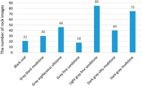
FIGURE 1. The specific numbers of different rock images.
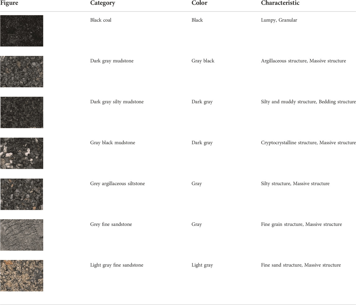
TABLE 1. The characteristics of seven types of rocks.
Datasets in deep learning are usually divided into the training set, validation set and test set, and different data subsets have different functions in model training. The training set is used to input data into the model to obtain results, then compare with the data labels to calculate the loss function, and finally update the parameters of the model through backpropagation to improve the performance of feature extraction and classification, so the training set accounts for the largest amount of data. The validation set is used to improve the training efficiency of the model. If the various hyperparameters are set or the model design is not reasonable when the model is under training, the model can respond to the accuracy of the validation set through the output, and then stop the training and make improvements in time. After the model is trained, the performance of the model can be evaluated using the test set. Similarly, the rock image dataset is randomly partitioned into the training set, validation set, and test set. If the ratio of the training set and validation set is too large, the model may overlearn and the model training time will grow, increasing the burden of model training, but a small ratio may also lead to model undertraining. The proportion of training, validation, and testing images in each label is set to 80%, 15%, and 5%, respectively. The dataset structure is shown in Table 2.
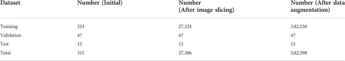
TABLE 2. Details of the rock dataset.
3 Methods
In order to fully extract the textural characteristics of different rocks, a rock image classification method based on the pre-trained residual neural network generated from transfer learning is proposed. Figure 2 presents the flowchart of the methods in this research.
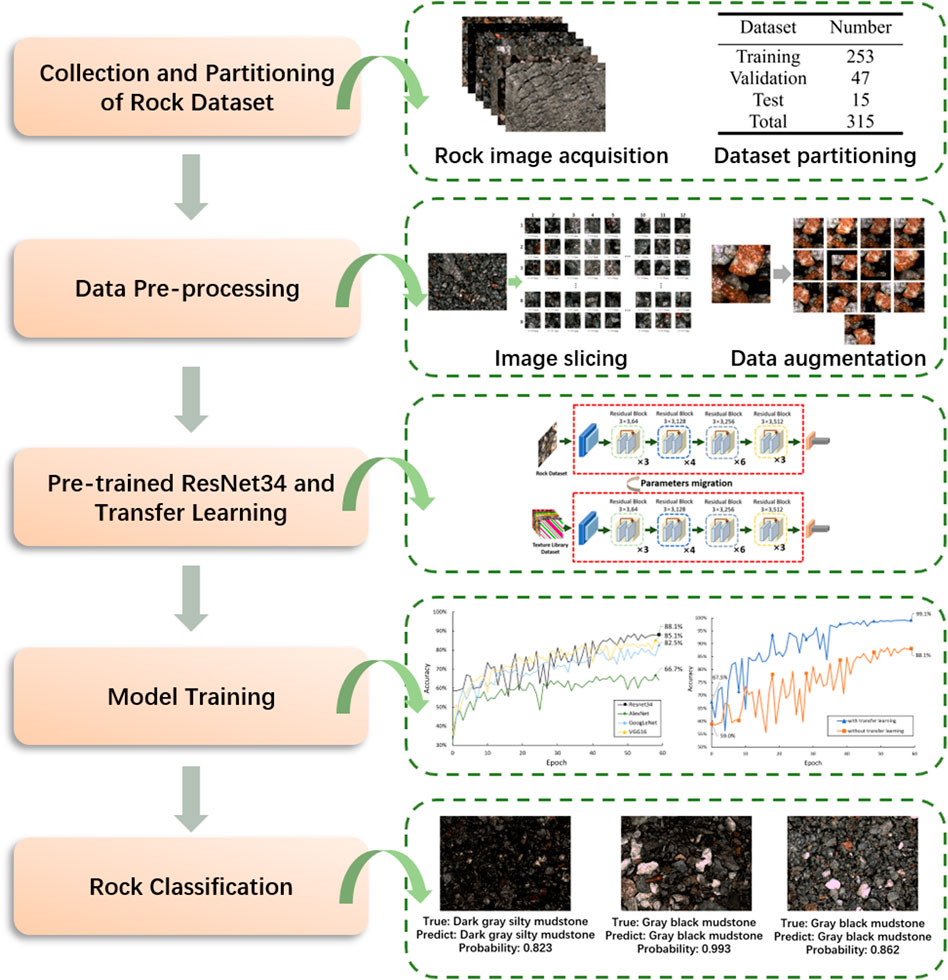
FIGURE 2. Flowchart of the methods.
3.1 The architecture of ResNet-34
Deep convolutional neural networks have made remarkable achievements in image classification, object detection, semantic segmentation and other fields. With the advancement of technology, more and more deep neural network models with better effects are constantly emerging (Luo and Wang, 2021). However, it is found that not the deeper the number of network layers, the better the model effect. The increase in network depth not only does not make the accuracy achieved by the traditional network higher, but also produces problems such as gradient disappearance, gradient explosion, and degradation.
Residual neural networks (i.e., ResNet) enable feature information from the input or learned in the shallow layers of the network to flow into the deeper layers by employing shortcut connections (He et al., 2016a). As the depth of the network increases, ResNet ensures the validity of gradient information by shortcut connections to prevent gradient disappearance and performance degradation caused by too deep layers of the network. Residual neural networks have achieved impressive results in image classification competitions such as ImageNet (He et al., 2016b) and MS COCO (Dai et al., 2016). In this study, ResNet is used to extract deep feature information from rock images to avoid the feature loss of the convolutional layer caused by gradient disappearance and gradient explosion in the process of information transmission.
ResNet consists of multiple residual blocks. The residual block not only has sequential convolutional layers, but also skips some convolutional layers through shortcut connections alongside the convolutional layers, and passes the data from the input residual block directly to the output, which is added with the result of the operation through the convolutional layer. Each residual structural unit can be defined as follows:
Where
The residual block is shown in Figure 3. Shortcut connection skips two layers of 3 × 3 convolutional layer connected to the output. The output of the main line through the convolution operation is added to the input through the shortcut. Then the result is output through the ReLU activation function (Nair and Hinton, 2010).
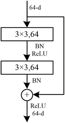
FIGURE 3. Examples of residual blocks with shortcut connections for the residual network (ResNet).
Figure 4 shows the ResNet architecture with 34 layers (i.e. ResNet34). The rock image input to resnet34 is first passed through a 7 × 7 convolutional layer and a 3 × 3 max pooling layer (both with a stride of 2), and then fed into 16 residual blocks. All of these residual blocks have a total of 32 layers. Finally, the network ends with an average pooling layer, a fully connected layer, and a softmax layer.
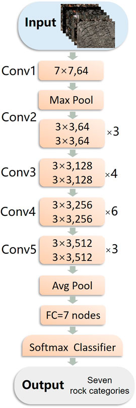
FIGURE 4. Detailed architectures for ResNet34.
3.2 Batch normalization
It is common for deep learning networks to consist of many layers. As the number of network layers increases, a significant deviation in data distribution across a layer will exacerbate, making it harder to optimize the model (Yan et al., 2020). Batch normalization (BN) can solve this problem well. Using batch normalization, data is divided into different groups and parameters are updated accordingly (Xiao et al., 2019). In the same group, the gradient direction is determined jointly, reducing randomness as the gradient declines. Furthermore, since the batch has fewer samples than the entire dataset, the amount of calculation has been significantly reduced. Batch normalization can avoid data offset because the batch normalization layer normalizes the input prior to the activation function.
In the ResNet34 rock image classification model we used, the BN is added before the ReLU activation function and after the convolutional layer. With the BN algorithm, parameter changes resulting from a different data distribution are minimized and the convergence speed during model training is accelerated. The formulas of batch normalization are as follows:
Where,
Through Eq. 3, the distribution of eigenvalues will be re-adjusted to a standard normal distribution and the eigenvalues are kept within the input-sensitive interval of the activation function, avoiding the disappearance of the gradient and speeding up the convergence.
3.3 ReLU activation function
The activation function is used to add nonlinear factors to the model because linear models are less expressive. In the absence of activation functions, the input of each layer node in the network is a linear function of the output of the upper layer, that is, inputs and outputs are linearly correlated (Liu et al., 2022). After adding the activation function, it is possible to apply neural networks to many nonlinear models arbitrarily because they can approach many nonlinear functions arbitrarily. As a result of the ReLU activation function, neurons are activated nonlinearly based on the feature map of the convolution layer output, enabling better learning by avoiding overfitting (Ran et al., 2019).
For each convolutional layer of ResNet34, the ReLU activation function is used:
Where
3.4 Softmax classifier
Softmax classifier is used in the establishment of the rock classification model. The input rock images can be converted into the corresponding category possibilities by the softmax classifier (Pham and Shin, 2020). At the end of ResNet34, the softmax classification function is added after the fully connected layer of the network, so that the output of the network is a one-dimensional vector of size 7, which represents the seven types of rocks to be classified in this study. The seven values in each one-dimensional vector reflect the rock class probability to which the input image belongs, so the sum of the seven values is 100%. The formula is as follows:
Where,
3.5 Adaptive moment estimation
Adaptive moment estimation (Adam) is a stochastic optimization algorithm based on the adaptive estimation of low-order moments (Hang et al., 2019; Yang et al., 2019). The algorithm adaptively adjusted the learning rate update parameters through the first moment estimation and the second moment estimation of the gradient. In the past, many conventional deep neural networks use stochastic gradient descent algorithm (SGD), which iteratively updates the weights of the neural network until it reaches the global optimal solution. However, the model using SGD algorithm has a slow convergence speed in the early stage, and it is prone to decline in accuracy. The Adam algorithm is improved on the basis of SGD algorithm. The learning rate during network training is usually kept constant when using an optimization algorithm such as SGD, but Adam optimizes the network by iteratively updating the weights of the neural network and adaptively adjusting the learning rate as the network is trained, which makes the network converge faster and learn better.
In order to adjust the parameters of the rock classification model more efficiently and make it converge faster during training, Adam is chosen as the optimization algorithm. The updating formulas of Adam algorithm are as follows:
Where,
3.6 Transfer learning
Training convolutional neural networks usually require very large labeled datasets to achieve high accuracy. However, it is often difficult to obtain such data and it takes a lot of time to label the data. Due to the existence of these difficulties, the transfer learning method used in many studies to solve the cross-domain image classification problem has proven very effective. Transfer learning considers the correlation between different tasks, so that the knowledge obtained in the previous task can be directly applied to the new task through small transformation or even without any modification. Transfer learning is conducive to the construction of the mathematical model of the target task and reduces the dependence on the target task dataset (Gao et al., 2021). At present, the more complete convolutional neural networks such as VGG, AlexNet, GoogLeNet and so on are pre-trained on the public image dataset of computer vision (Dabrowski and Michalik, 2017; Ali et al., 2020).
Since the model needs multiple rounds of iteration in the training process, and the number of rock pictures in this study is small, it will lead to the overfitting problem and low classification accuracy of the model. Consequently, transfer learning is a viable strategy (Figure 5). Given a labelled source domain
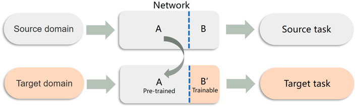
FIGURE 5. Demonstration of transfer learning.
As shown in Figure 6, transfer learning is used to optimize the rock image classification. Transfer learning in the rock image classification model includes pre-training and fine-tuning. Firstly, the ResNet34 model is pre-trained on the Texture Library dataset, the rock dataset is used to fine-tune the ResNet34 model afterwards.
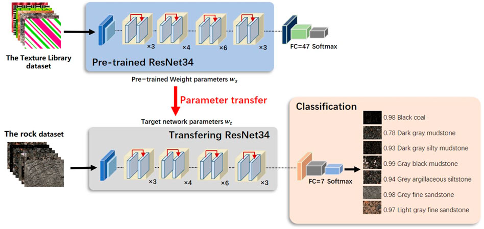
FIGURE 6. Schematic diagram of transfer learning in rock classification.
The supervised learning architecture is used for pre-training. Pre-training usually requires a large enough dataset to help the model learn common features, and the learned features are parameterized to be ported to similar tasks for reuse (Zhu et al., 2021; Yi et al., 2022). The Texture Library dataset which contains 47 texture types total of 78,960 images is selected as the source domain for pre-training (Figure 7). The rock dataset and the Texture Library dataset are not identical, but the images of both have similar texture features, so the two dataset domains are related. Using the Texture Library dataset as the input of the pre-trained model for ResNet34, the characteristics of rocks can be well reflected. Therefore, it is reasonable to adopt the ResNet34 model pre-trained with the Texture Library dataset for rock image classification.
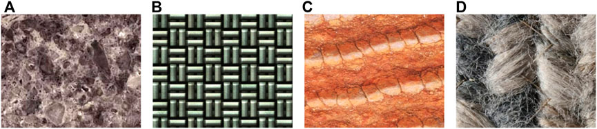
FIGURE 7. Example images of the Texture Library dataset: (A) Marble, (B) Brick grain, (C) Soil grain, (D) Bean vermicelli.
For fine-tuning, the parameters trained on the Texture Library dataset are used as initial values. The parameters of each layer of the network are frozen except for the last fully connected layer, and then input rock dataset and retrain the last fully connected layer to complete the fine-tuning.
In this study, the transfer learning method based on ResNet34 was applied to the rock image classification model. The ResNet34 pre-training weight parameters obtained by pre-training on the texture dataset are fine-tuned to speed up the convergence speed of the rock image classification network training, and spend less time training to obtain a model that can classify rock images. Transfer learning is used to simplify the original image training process, making the model learning more efficient and flexible.
4 Experiments and results
4.1 Data pre-processing
In the rock dataset used in the experiment, the number of rock images is too small and the pixel is too large. The number of samples in each rock category is uneven, which will affect the recognition accuracy, so the rock training set is preprocessed.
4.1.1 Image slicing
Image information is composed of the spatial arrangement of pixels, so the features of an image are mainly represented by local adjacent pixels (Su et al., 2020). Large-scale images can represent more image detail information, so that the differences between images are more obvious. Image classification should make full use of image detail information. Therefore, we use the image slicing method to slice the 253 training sets at first. The original rock images acquired from the industrial camera contain 4,096 × 3,000 pixels and are sliced into 9 rows and 12 columns, meaning that each original image is divided into 108 sub-images. The size of each sub-image is 322 × 322 pixels. The original image and its cut part images are shown in Figure 8A.
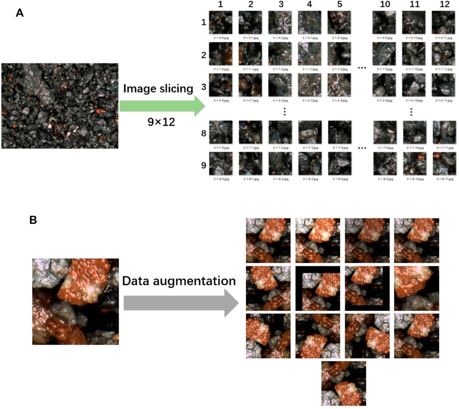
FIGURE 8. Data pre-processing of rock images: (A) Image slicing (B) Data augmentation.
4.1.2 Data augmentation
rAfter image slicing, the training dataset is expanded to 27,324 images. The dataset used consisted of a relatively small number of images for training network. The data augmentation used in this study to expand the dataset were rotation, horizontal flip, vertical flip, blur, movement, brightness adjustment and Gaussian noise addition. The schematic of the data augmentation is shown in Figure 8B. The total number of training sets reached 382,536 by applying these transformations which fully expanded the original training set. The number of training set after pre-processing is also shown in Table 2.
4.1.2.1 Image resizing
Resizing changes the distance between different pixels in the image, typically along the x-axis and y-axis, and the matrix expression for image resizing is as follows:
Where,
4.1.2.2 Image rotation
Rotation is the process of rotating an image around a point to form a new image. The pixel values of the image before and after rotation remain unchanged. When the selected rotation point is the coordinate origin, the matrix expression for image rotation is as follows:
Where,
4.1.2.3 Image movement
The matrix expression of image movement is as follows:
Where,
4.1.2.4 Image flip
The matrix expression for the horizontal flip is as follows:
The matrix expression for the vertical flip is as follows:
Where w is the width of the image and h is the height of the image.
4.1.2.5 Brightness change
The change of image brightness belongs to the pixel transformation of the image, that is, the linear transformation is performed on each point of the two-dimensional matrix represented by the image. The transformation formula is as follows:
Where
4.1.2.6 Noise addition
Due to the random interference of the external environment such as light and dust, the acquired rock image will contain noise. In order to simulate the real environment, Gaussian noise is added to the image. The probability density function of Gaussian noise is as follows:
Where
4.2 Evaluation metrics
The primary measures used to evaluate training effectiveness are classification accuracy and loss value. The classification accuracy is the percentage of the currently trained images that are accurately classified. It is formulated by Eq. 19:
Where,
Through the calculation of the loss function, the parameters of our model are updated. The goal is to reduce the optimization error, that is, to reduce the empirical risk of the model under the joint effect of the loss function and the optimization algorithm (Chen et al., 2021). The cross-entropy is used as the loss function to evaluate the difference between the predicted value and the true value (Li et al., 2020). The loss value in this work is calculated by cross entropy, as follows:
Where,
4.3 Experiment details
The device information used in the experiment is as follows: the CPU model is Intel Xeon Silver 4,110 with 16 GB memory, and the GPU model is GeForce RTX 2080Ti with 11G memory. Windows10 was used as the operating system and Python 3.6 was used as the programming language. The deep learning framework is Pytorch, version 10.1 for CUDA, and version 7.6.5 for CuDNN.
The activation function selects the ReLU function. The optimizer selects is Adam. The learning rate is set to 0.001. The number of training epochs is 60 and the batch size is set to 16.
Different degrees of data preprocessing methods were used to conduct ablation experiments to explore the effectiveness of each preprocessing method. Resnet34 and three other different neural networks were trained to explore which worked best. The Texture Library dataset is selected as the source domain for transfer learning. The model parameter files are obtained after training. The other layers of the Resnet34 network are frozen except for the structural parameters of the fully connected layer. The pre-trained weights obtained from training on the texture dataset are loaded when the network is trained with the rock dataset. The prediction results are compared with the true label in each step so that the classification accuracy and loss value are both calculated to upload to the TensorBoard visual training tool.
4.4 Results analysis
4.4.1 The effectiveness of data pre-processing
The original data in this paper has been pre-processed by image slicing and data augmentation. In order to verify the effectiveness of data pre-processing, we conduct ablation experiments. The ResNet34 network was used to conduct four groups of experiments on different training sets: 1) no data pre-processing is used; 2) using image slicing; 3) using data augmentation; 4) using image slicing and data augmentation both on the training set. The highest accuracy achieved by each method in 60 epochs is shown in Table 3.
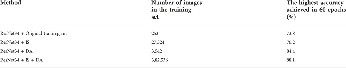
TABLE 3. Comparison of training results for different data preprocessing methods.
After different degrees of image pre-processing, the classification accuracy of the network is improved in different degrees. Compared with the original training set, the accuracy of the training set after image slicing and data augmentation is improved by 14.3%. The result indicates that pre-processing of small sample data sets can make the network extract more comprehensive rock features and improve the generalization ability of the model. And it proves that the data pre-processing method in this paper can improve the overall accuracy of the classification network.
4.4.2 The effectiveness of residual networks
Four different network models to apply to rock classification in order to compare which network has the best effect are trained respectively. The training is visualized in the Pytorch framework using the TensorBoard tool.
Figure 9 illustrates the loss and accuracy changes for four deep learning methods (AlexNet, VGG16, GoogleLeNet, and ResNet34) as experiment steps increase. It shows that each of the four convolutional neural networks converges as the training process of rock image classification proceeds. In addition, it can be reflected from Figure 9A that the rock accuracy of the four networks from high to low is ResNet34, VGG16, GoogLeNet, and AlexNet. While the loss values (Figure 9B) are the opposite, from large to small are AlexNet, GoogLeNet, VGG16, and ResNet34.
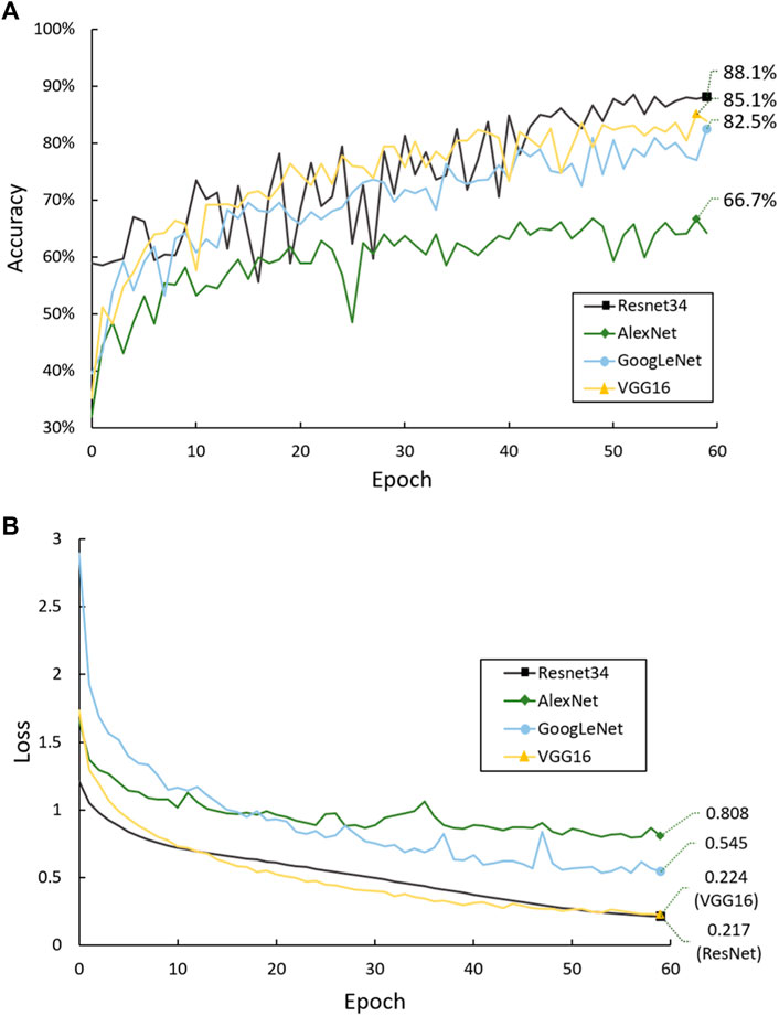
FIGURE 9. The accuracy (A) and the loss (B) values of four different models over different epochs.
The residual neural network has the highest accuracy and the lowest loss value, which is because the residual network uses residual structure to solve the model degradation problem of deep neural network. In conclusion, the ResNet34 network performs better than other networks in rock image classification.
4.4.3 The effectiveness of transfer learning
In order to explore whether the model using transfer learning performs better, the rock classification model using transfer learning method and the model without transfer learning method are trained respectively. The change of accuracy and loss value during the training process is shown in Figure 10. Compared with the training results with and without transfer learning, the first accuracy and the highest accuracy of the training epochs and the corresponding loss value are shown in Table 4. Combined with the graph, it can be observed that the model training without transfer learning has a low accuracy of 59.0% in the early stage. The highest accuracy reaches 88.1% after 60 epochs and the corresponding loss value is 0.217. In the model using transfer learning, the accuracy of the first epoch reaches 67.5% and the accuracy fluctuates slightly during the training process. The highest accuracy reached 99.1% which achieves an 11% improvement compared with the model without transfer learning, and the corresponding loss value is 0.085.
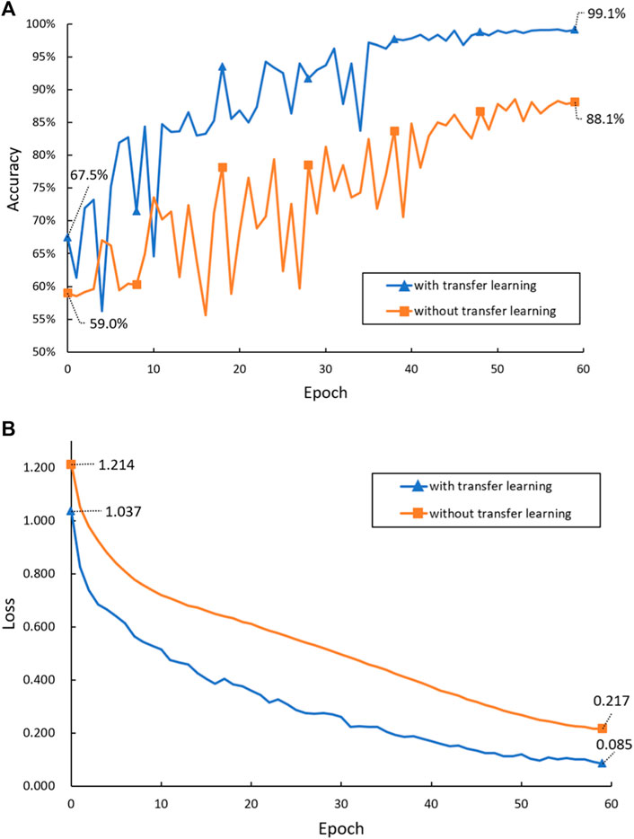
FIGURE 10. The accuracy (A) and the loss (B) values of the models over different epochs.
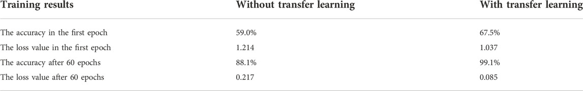
TABLE 4. Comparison of training results with or without transfer learning.
The accuracy and loss values reflect that the effect of the network model trained by transfer learning is obviously better than the original model. The model using transfer learning has high initial accuracy and high final accuracy. This is because the pre-training network based on the Texture Library dataset has learned rich texture spatial structure features and morphological correlation. The parameters of the pre-training model can be directly used in the model training, which can save training time and improve the precision of rock classification.
4.4.4 Reality testing
A total of 15 images covering 7 types of rocks from the testing dataset were classified by the model which had the weights with the highest accuracy using transfer learning method. The rock images to be recognized were fed into the rock prediction program, and the classification result was given in the form of names and probabilities. The test result of rock classification is shown in Figure 11. All 15 images were correctly predicted with probabilities above 82%, and most of them were even above 95%.
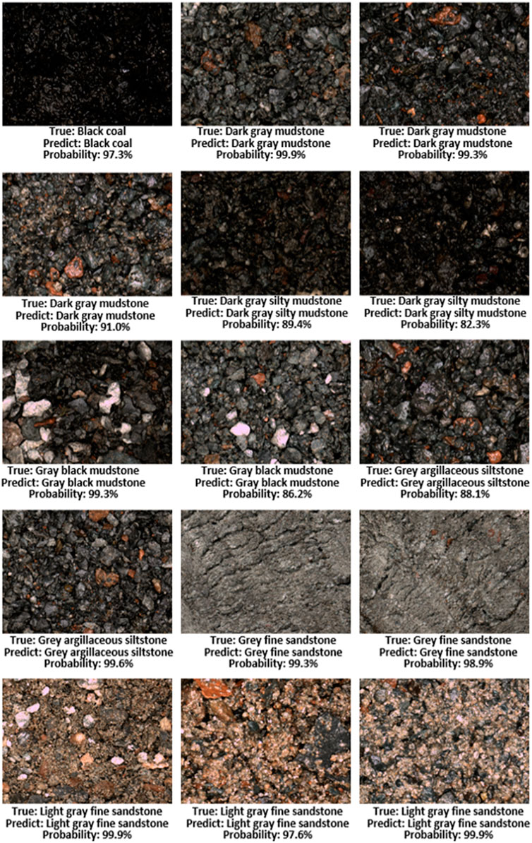
FIGURE 11. The test result of rock classification.
Since the shooting angle and distance of rocks in the survey site are not fixed, the classification effect of rock images with different views is tested in this paper. Considering that the imaging resolution of each camera is not the same in practical applications, it is also necessary to test the effect of different resolutions of images on the rock classification results.
To simulate the camera changes at different resolutions, the image resolution was changed while keeping the view of the image unchanged. The original images of the test set are all 4,096 × 3,000 pixels. The original 15 test set images were down sampled multiple times to reduce the image resolution. The average accuracy of classifying 15 rock images is used as the evaluation criterion, and the experimental results are shown in Figure 12A.
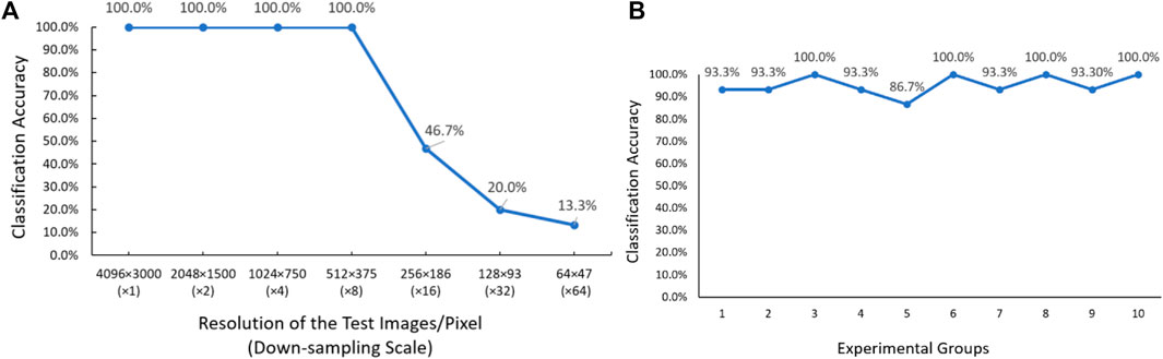
FIGURE 12. The accuracy and the loss the influence of image resolution on the classification results (A) and the influence of the change of image field of view on the classification results (B).
It can be seen that the classification accuracy starts to suffer when the image is below 512 × 375 pixels. This is because the images of the original training set are processed to 322 × 322 pixels through image slicing in the previous data preprocessing, so the network can accurately identify the input images with a resolution higher than 322 × 322. When the resolution of an image is lower than 322 × 322 pixels, the reduction of image features affects the rock classification results.
In order to simulate the change in the distance between the camera and the rock sample, the view of the image is changed while keeping the image resolution unchanged. The above experimental results show that the rock classification model can accurately classify rocks when the input image is in the pixels range of 4,096 × 3,000 to 512 × 375. However, the accuracy starts to decrease after pixels are below 512 × 375. Therefore 512 × 375 pixels are used as the minimum image resolution limit. After arbitrarily cropping an image with the same proportion as the original rock image and greater than 512 × 375 pixels, a random brightness change is added to simulate the field light change. And it is down sampled to 512 × 375 pixels to control the image resolution consistency, then input into the classification network for classification test. A total of 10 tests were performed, and the test set for each classification was 15 images. The experimental results are shown in Figure 12B.
The accuracy of rock classification does not change significantly due to the data pre-processing we have used. The pre-processing can improve the robustness and generalization of the model. Therefore, the model can adapt to the changes of different resolutions, shooting angles and shooting scenes. It indicates that the model learns more about rock lithological features with the increase in data volume. This result also shows that the model has good robustness and generalization ability.
4.4.5 Comprehensive analysis
Ablation experiments were conducted to verify the effectiveness of the data preprocessing done in this paper. Since the original rock data set is too small, image segmentation and data augmentation can significantly improve the accuracy of rock classification. The effectiveness of residual neural networks is verified by the comparative experiment of AlexNet, VGG16, GoogLeNet, and ResNet34. The effectiveness of transfer learning is verified by the comparative experiment between transfer learning and non-transfer learning. The practical usability of the rock classification model was verified by testing 15 images containing all seven types of rocks. All 15 images were correctly predicted with probabilities above 82%, and most of them were even above 95%. By simulating and testing the actual situation of camera view changes and resolution changes, it is verified that the model has good robustness, slight scene changes will not affect the accuracy of rock classification, and the effectiveness of data preprocessing is also shown. These experimental results indicate that the model using transfer learning with the pre-trained residual neural network has higher classification accuracy and good generalization ability.
5 Deployment and application of rock classification network
Geological survey work often needs to be carried out on the construction site or in off-line conditions. Geological investigators need to carry all kinds of geological exploration equipment, such as GPS measurement, positioning instruments, measuring instruments and so on. It is inconvenient to take equipment with a certain weight and volume such as workstations, and it is impossible to obtain timely feedback on rock types through the network to guide the following investigation. Deploying the rock image classification model proposed in this paper to the embedded end device can effectively solve this problem.
In this paper, rock image classification is shifted from theoretical research to practical applications. The trained rock classification network model is transplanted to Nvidia Jetson TX2 embedded platform, the TensorRT inference optimizer is used to accelerate the model, and the front-end interface that integrates all aspects of the system is developed, which makes the system both portable and easy to use, and meets the requirements of geological survey field deployment.
5.1 Design of rock classification system
A rock classification system is constructed based on the designed rock image classification model. The overall framework is shown in Figure 13A, and the specific functions of the system are as follows: 1) Get an image of the rock. Images are acquired in real-time from connected industrial cameras, or rock images are fetched from local data. Real-time detection and local data acquisition are introduced to meet the requirements of the geological survey sites. 2) Rock image preprocessing. The rock images that need to be input into the classification network are preprocessed first, the brightness of the rock images that are too bright or too dark is corrected, and the rock images are smoothed to remove the sharp noise, reduce the level of detail, and enhance the recognition effect of the image under different proportions. The preprocessed rock image is used as the input image of the subsequent classification network, and improving the image identifiability is beneficial to improve the accuracy of rock classification. 3) Rock image classification. The rock classification network is loaded, and the preprocessed rock images are input for inference to obtain the rock classification results. If it is necessary to extend the rock category or use a better-trained rock model, the rock classification model can be updated by replacing the original model weights with the newly trained model weights. 4) The obtained rock classification results are stored or displayed on the visual interface.
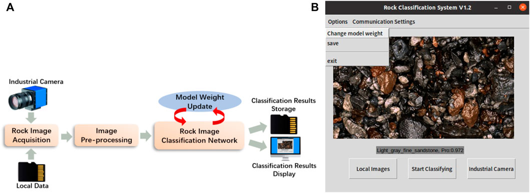
FIGURE 13. The rock classification system: (A) System framework diagram (B) Visual interface.
5.2 System deployment
The preliminary development of the rock classification model proposed in this paper is carried out on the PC side, but the size of the PC side is huge, and it is not suitable for deployment in the industrial survey site. In contrast, embedded devices with deep learning computing capabilities are more in line with the needs of geological exploration. To consider the practical application, we port the algorithm from the PC to the embedded platform. Considering that there is usually no network support in the actual survey site, this paper adopts the offline deployment mode. After the model is trained in the PC server in advance, it is deployed on the embedded device.
This paper implements the deployment process of the rock classification network on Nvidia Jetson TX2. Nvidia Jetson TX2 is an embedded AI computing device launched by Nvidia Corporation. Its GPU adopts Nvidia Pascal architecture, has 8 GB memory and 32 GB storage space, and is equipped with a variety of standard hardware interfaces. Jetson TX2 is compact and energy efficient, making it ideal for smart edge devices such as robots, drones, and smart cameras.
The deep learning network model trained on the PC usually has a large number of parameters, and it is easy to cause problems of slow inference speed and poor real-time performance of the model when deployed on embedded devices with weak performance. In order to accelerate the reasoning of the model on embedded devices, the TensorRT framework developed by Nvidia is used to accelerate the reasoning. NVIDIA TensorRT is a special optimizer for neural network inference, which is mostly used in image classification, object detection and other fields. It uses a scheme to optimize the trained model, which can provide low latency and high throughput for deep learning model inference applications deployed in the production environment.
The steps for porting the rock classification algorithm are as follows: First, set up the software development environment on Jetson TX2 and install the libraries that the application depends on to run. Since the trained model is generated by the Pytorch framework and cannot be directly applied to the TensorRT framework, the Pytorch model is first converted to the ONNX (OpenNeural Network Exchange) format to make it suitable for the TensorRT framework. ONNX is a standard format for representing deep learning models that can be transferred between different frameworks (Chang et al., 2020). Many model formats can only be converted to ONNX to work with the TensorRT framework. Finally, the visual interface integrating each function was developed.
The user interface design of this paper takes into account that this system is mainly provided for geological exploration personnel. From the perspective of practical application, the code is encapsulated, and the PYQT module in Python is used for visual interface design. The rocks are classified through the visual interface, and the classification results are displayed and saved, which reduces the threshold of use and facilitates the use of engineers. The main interface is shown in Figure 13B.
6 Conclusion
In this study, a deep residual neural network model with transfer learning method is proposed to classify rock images quickly and accurately. The dataset is expanded by image slicing and data augment, and the Resnet34 is pre-trained by the Texture Library dataset for transfer learning. The comparative analysis shows that the model using transfer learning in ResNet34 structure for rock image classification has an excellent effect, and the classification accuracy is as high as 99.1%, which achieves an 11% improvement compared with the model without transfer learning. The excellent performance of the rock classification model is mainly due to the introduction of the residual module and the application of transfer learning. The pre-trained network based on the texture dataset learns rich texture spatial structure features and morphological correlation. Finally, a rock classification system is designed and deployed on embedded devices to meet geological survey tasks. The system extracts feature by the convolutional neural network without manual operation, which reduces the influence of subjective factors. This system has low requirements for rock image acquisition configuration and environment, which fully demonstrates its robustness and generalization ability.
Our future study will further increase the number of rock categories and ensure that the classification accuracy is further improved when more rock types are added, as the types and number of rock datasets in this paper are limited due to the limitations of shooting conditions.
Data availability statement
Publicly available datasets were analyzed in this study. This data can be found here: http://www.olegvolk.net/gallery/various/textures.
Author contributions
WC was responsible for the implementation of the proposed method and the writing of the manuscript. LS was responsible for making important revisions to the manuscript to make it clearer and more reasonable, and proposed ideas for method improvement. XC was responsible for constructing the initial research idea and analyzing the rationality of the experimental results. ZH was responsible for the grammar checking and language polishing of the manuscript.
Funding
This work is financially supported in part by the National Natural Science Foundation of China under Grant 61903315 and the Foundation for Science and Technology Cooperation Program of Longyan under Grant 2020LYF16004; in part by the Natural Science Foundation of the Department of Science and Technology of Fujian Province under Grant 2022J011255.
Acknowledgments
The authors thank all editors and reviewers for their comments and suggestions. For this study, special thanks to the GuangDong TipDM Intelligent Technology Co., Ltd. for providing the data.
Conflict of interest
The authors declare that the research was conducted in the absence of any commercial or financial relationships that could be construed as a potential conflict of interest.
Publisher’s note
All claims expressed in this article are solely those of the authors and do not necessarily represent those of their affiliated organizations, or those of the publisher, the editors and the reviewers. Any product that may be evaluated in this article, or claim that may be made by its manufacturer, is not guaranteed or endorsed by the publisher.
References
Ali, S. B., Wate, R., Kujur, S., Singh, A., and Kumar, S. (2020). “Wall crack detection using transfer learning-based cnn models,” in 2020 IEEE 17th India Council International Conference (INDICON) (IEEE), 1–7.
Bai, L., Wei, X., Liu, Y., Wu, C., and Chen, L. (2019). Rock thin section image recognition and classification based on vgg model. Geol. Bull. China 38, 2053–2058.
Bai, L., Yao, Y., Li, S., Xu, D., and Wei, X. (2018). Mineral composition analysis of rock image based on deep learning feature extraction. China Min. Mag. 27, 178–182.
Chang, Y.-M., Liao, W.-C., Wang, S.-C., Yang, C.-C., and Hwang, Y.-S. (2020). A framework for scheduling dependent programs on gpu architectures. J. Syst. Archit. 106, 101712. doi:10.1016/j.sysarc.2020.101712
Chen, J., Yang, T., Zhang, D., Huang, H., and Tian, Y. (2021). Deep learning based classification of rock structure of tunnel face. Geosci. Front. 12, 395–404. doi:10.1016/j.gsf.2020.04.003
Cheng, G., Guo, W., and Fan, P. (2017). Study on rock image classification based on convolution neural network. J. Xi’an Shiyou Univ. Nat. Sci. Ed. 32, 116–122.
Dabrowski, M., and Michalik, T. (2017). How effective is transfer learning method for image classification. Position papers of the Federated Conference on Computer Science and Information Systems, 3–9.
Dai, J., He, K., and Sun, J. (2016). “Instance-aware semantic segmentation via multi-task network cascades,” in Proceedings of the IEEE conference on computer vision and pattern recognition, 3150–3158.
Falivene, O., Auchter, N. C., de Lima, R. P., Kleipool, L., Solum, J. G., Zarian, P., et al. (2022). Lithofacies identification in cores using deep learning segmentation: Turbidite deposits (gulf of Mexico and north sea) and the geoscientists role. AAPG Bull.
Fan, G., Chen, F., Chen, D., Li, Y., and Dong, Y. (2020). A deep learning model for quick and accurate rock recognition with smartphones. Mob. Inf. Syst. 2020, 1–14. doi:10.1155/2020/7462524
Feng, Y., Gong, X., Xu, Y., Xie, Z., Cai, H., and Lv, X. (2019). Lithology recognition based on fresh rock images and twins convolution neural network. Geogr. Geo-Information Sci. 35, 89–94.
Gao, M., Qi, D., Mu, H., and Chen, J. (2021). A transfer residual neural network based on resnet-34 for detection of wood knot defects. Forests 12, 212. doi:10.3390/f12020212
Gonçalves, L. B., and Leta, F. R. (2010). Macroscopic rock texture image classification using a hierarchical neuro-fuzzy class method. Math. problems Eng. 2010, 1–23. doi:10.1155/2010/163635
Guo, W., Dong, C., Lin, C., Wu, Y., Zhang, X., and Liu, J. (2022). Rock physical modeling of tight sandstones based on digital rocks and reservoir porosity prediction from seismic data. Front. Earth Sci. (Lausanne). 10, 932929. doi:10.3389/feart.2022.932929
Hang, J., Zhang, D., Chen, P., Zhang, J., and Wang, B. (2019). Classification of plant leaf diseases based on improved convolutional neural network. Sensors 19, 4161. doi:10.3390/s19194161
He, K., Zhang, X., Ren, S., and Sun, J. (2016a). “Deep residual learning for image recognition,” in Proceedings of the IEEE conference on computer vision and pattern recognition, 770–778.
He, K., Zhang, X., Ren, S., and Sun, J. (2016b). “Identity mappings in deep residual networks,” in European conference on computer vision (Springer), 630–645.
Houshmand, N., GoodFellow, S., Esmaeili, K., and Calderón, J. C. O. (2022). Rock type classification based on petrophysical, geochemical, and core imaging data using machine and deep learning techniques. Appl. Comput. Geosciences 16, 100104. doi:10.1016/j.acags.2022.100104
Hu, Q., Ye, W., Wang, Q., and Chen, Y. (2020). Recognition of lithology with big data of geological images. J. Eng. Geol. 28, 1433–1440.
Iglesias, J. C. Á., Santos, R. B. M., and Paciornik, S. (2019). Deep learning discrimination of quartz and resin in optical microscopy images of minerals. Miner. Eng. 138, 79–85. doi:10.1016/j.mineng.2019.04.032
Imamverdiyev, Y., and Sukhostat, L. (2019). Lithological facies classification using deep convolutional neural network. J. Petroleum Sci. Eng. 174, 216–228. doi:10.1016/j.petrol.2018.11.023
Karimpouli, S., and Tahmasebi, P. (2019). Segmentation of digital rock images using deep convolutional autoencoder networks. Comput. geosciences 126, 142–150. doi:10.1016/j.cageo.2019.02.003
Koeshidayatullah, A., Al-Azani, S., Baraboshkin, E. E., and Alfarraj, M. (2022). Faciesvit: Vision transformer for an improved core lithofacies prediction. Front. Earth Sci. (Lausanne). 10, 992442. doi:10.3389/feart.2022.992442
Li, J., Zhang, L., Wu, Z., Ling, Z., Cao, X., Guo, K., et al. (2020). Autonomous martian rock image classification based on transfer deep learning methods. Earth Sci. Inf. 13, 951–963. doi:10.1007/s12145-019-00433-9
Liang, Y., Cui, Q., Luo, X., and Xie, Z. (2021). Research on classification of fine-grained rock images based on deep learning. Comput. Intell. Neurosci. 2021, 1–11. doi:10.1155/2021/5779740
Liu, Y.-Z., Ren, S.-F., and Zhao, P.-F. (2022). Application of the deep neural network to predict dynamic responses of stiffened plates subjected to near-field underwater explosion. Ocean. Eng. 247, 110537. doi:10.1016/j.oceaneng.2022.110537
Luo, Y., and Wang, Z. (2021). “An improved resnet algorithm based on cbam,” in 2021 International Conference on Computer Network Electronic and Automation (ICCNEA), Xi'an, China, 24-26 September 2021 (IEEE), 121–125.
Młynarczuk, M., Górszczyk, A., and Ślipek, B. (2013). The application of pattern recognition in the automatic classification of microscopic rock images. Comput. Geosciences 60, 126–133. doi:10.1016/j.cageo.2013.07.015
Nair, V., and Hinton, G. E. (2010). “Rectified linear units improve restricted Boltzmann machines,” in Icml.
Pan, J. (2017). “Review of metric learning with transfer learning,” in AIP Conference Proceedings (Melville, NY: AIP Publishing LLC), 020040.1864.
Patel, A. K., and Chatterjee, S. (2016). Computer vision-based limestone rock-type classification using probabilistic neural network. Geosci. Front. 7, 53–60. doi:10.1016/j.gsf.2014.10.005
Pham, C., and Shin, H.-S. (2020). A feasibility study on application of a deep convolutional neural network for automatic rock type classification. Tunn. Undergr. space 30, 462–472.
Ran, X., Xue, L., Zhang, Y., Liu, Z., Sang, X., and He, J. (2019). Rock classification from field image patches analyzed using a deep convolutional neural network. Mathematics 7, 755. doi:10.3390/math7080755
Ru, Z., and Jiong, M. (2019). Identification and evaluation of logging methods for quartz sandstone gas reservoir in yulin gas field. J. Liaoning Univ. Petroleum Chem. Technol. 39, 65.
Sharif, H., Ralchenko, M., Samson, C., and Ellery, A. (2015). Autonomous rock classification using bayesian image analysis for rover-based planetary exploration. Comput. Geosciences 83, 153–167. doi:10.1016/j.cageo.2015.05.011
ShuTeng, X., and YongZhang, Z. (2018). Artificial intelligence identification of ore minerals under microscope based on deep learning algorithm. Acta Petrol. Sin. 34, 3244–3252.
Singh, N., Singh, T., Tiwary, A., and Sarkar, K. M. (2010). Textural identification of basaltic rock mass using image processing and neural network. Comput. Geosci. 14, 301–310. doi:10.1007/s10596-009-9154-x
Su, C., Xu, S.-j., Zhu, K.-y., and Zhang, X.-c. (2020). Rock classification in petrographic thin section images based on concatenated convolutional neural networks. Earth Sci. Inf. 13, 1477–1484. doi:10.1007/s12145-020-00505-1
Wang, Y., and Sun, S. (2021). Image-based rock typing using grain geometry features. Comput. Geosciences 149, 104703. doi:10.1016/j.cageo.2021.104703
Xiao, D., Le, B. T., and Ha, T. T. L. (2021). Iron ore identification method using reflectance spectrometer and a deep neural network framework. Spectrochimica Acta Part A Mol. Biomol. Spectrosc. 248, 119168. doi:10.1016/j.saa.2020.119168
Xiao, Q., Li, W., Kai, Y., Chen, P., Zhang, J., and Wang, B. (2019). Occurrence prediction of pests and diseases in cotton on the basis of weather factors by long short term memory network. BMC Bioinforma. 20, 1–15. doi:10.1186/s12859-019-3262-y
Yan, Q., Yang, B., Wang, W., Wang, B., Chen, P., and Zhang, J. (2020). Apple leaf diseases recognition based on an improved convolutional neural network. Sensors 20, 3535. doi:10.3390/s20123535
Yang, B., Wang, M., Sha, Z., Wang, B., Chen, J., Yao, X., et al. (2019). Evaluation of aboveground nitrogen content of winter wheat using digital imagery of unmanned aerial vehicles. Sensors 19, 4416. doi:10.3390/s19204416
Yi, X., Li, H., Zhang, R., Gongqiu, Z., He, X., Liu, L., et al. (2022). Rock mass structural surface trace extraction based on transfer learning. Open Geosci. 14, 98–110. doi:10.1515/geo-2022-0337
Zeng, X., Xiao, Y., Ji, X., and Wang, G. (2021). Mineral identification based on deep learning that combines image and mohs hardness. Minerals 11, 506. doi:10.3390/min11050506
Zhang, Y., Li, M., and Han, S. (2018). Automatic identification and classification in lithology based on deep learning in rock images. Yanshi Xuebao/Acta Petrol. Sin. 34, 333–342.
Keywords: deep learning, image recognition, rock classification, transfer learning, convolutional neural network
Citation: Chen W, Su L, Chen X and Huang Z (2023) Rock image classification using deep residual neural network with transfer learning. Front. Earth Sci. 10:1079447. doi: 10.3389/feart.2022.1079447
Received: 25 October 2022; Accepted: 22 November 2022;
Published: 16 January 2023.
Edited by:
Abbas Maghsoudi, Amirkabir University of Technology, IranReviewed by:
Kalpana Bhatt, Purdue University, United StatesSadegh Karimpouli, University of Zanjan, Iran
Copyright © 2023 Chen, Su, Chen and Huang. This is an open-access article distributed under the terms of the Creative Commons Attribution License (CC BY). The use, distribution or reproduction in other forums is permitted, provided the original author(s) and the copyright owner(s) are credited and that the original publication in this journal is cited, in accordance with accepted academic practice. No use, distribution or reproduction is permitted which does not comply with these terms.
*Correspondence: Lumei Su, c3VsdW1laUAxNjMuY29t