Automatic velocity picking with restricted weighted k-means clustering using prior information

Automatic picking of seismic velocity can be performed using k-means clustering. In simple k-means clustering, the number of clusters needs to be predetermined, while the picking result is affected by the initial value of each cluster center. In this study, we present an unsupervised weighted k-means clustering velocity-picking method that picks the centers of the energy clusters instead of the geometric centers of the clusters. This method works on the semblance velocity spectrum and requires an initial velocity function and three user-defined thresholds to limit the search area. The number of cluster centers and their initial times are obtained according to a rectangular signal resulting from the three thresholds, while the initial velocities of the cluster centers can be subsequently obtained using their initial times and the initial velocity function. Inaccurate selection of thresholds may merge two clusters wrongly, in which case only a stronger event is selected. In the weighted k-means clustering algorithm, weights are calculated by using the amplitudes of the velocity points. Meanwhile, points far from the center are gradually removed to ensure that each cluster center coincides with the respective energy cluster center. We also propose a method for ignoring non-primary velocities, such as multiples, by removing points that create sudden changes in the slope of the reference velocity beyond a user-defined limit. The processing of the model and real data show that the proposed seismic velocity-picking method has high efficiency and picking accuracy.

1 Introduction

Velocity analysis and picking of seismic data are very important for conventional seismic processing, and significantly impact on static, velocity modeling, imaging, and inversions (Neidell and Taner, 1971; Fomel, 2009; Yuan et al., 2022). However, manual picking is not only labor-intensive, but also inefficient. To this end, scholars have proposed various automatic picking methods for seismic velocities. At present, automatic picking methods for seismic velocities mainly includes two types, namely optimization search methods and artificial intelligence velocity-picking methods. Optimization search methods determine the position with the maximum energy in the velocity spectrum according to actual geological conditions, and the position is identified as the selected velocity. Toldi (1989) proposed a method that takes the maximum superposition energy of the velocity spectrum as the objective function, used the conjugate gradient method to search for the maximum value, and finally realized automatic velocity picking. However, this method assumes that the model is linear and significantly disturbed by noise (Toldi, 1989). Zhang and coworkers implemented seismic velocity picking using a nonlinear optimization algorithm (Zhang, 1997; Zhang and Claerbout, 1998). Almarzoug and Ahmed. (2012) implemented an automatic velocity-picking methodology by treating the velocity-picking process as a variational problem. Lumley (1997) developed an automatic velocity-picking method using a Monte Carlo nonlinear fitting technique. Choi et al. (2010) developed an efficient automatic velocity-analysis algorithm by using bootstrapped differential semblance and Monte Carlo inversion. Usually, the optimization algorithm requires a priori constraints, with the initial velocity values having significant influence on the final calculation accuracy.

Artificial intelligence velocity-picking methods achieve velocity picking by identifying energy clusters in the velocity spectrum and include deep learning and cluster analysis methods (Schmidt, 1992). Fish and Kusuma. (1994) meshed the velocity spectrum, used a neural network to identify it, and eventually realized intelligent velocity picking. Zha (1996) combined a neural network with fuzzy mathematics, used fuzzy mathematics to perform boundary search and fuzzy clustering preprocessing on the velocity spectrum, and trained the neural network to automatically pick the velocity. Dong and He (1996) sorted the velocities of energy peaks according to the binary tree structure, formed a network input vector to train the neural network, and eventually realized automatic velocity picking. Traditional artificial neural networks required a large amount of calculations and could not achieve satisfactory results owing to the limitations of early computing resources. The improvement of computer performance allowed scholars to increase the breadth and depth of neural networks, thereby improving their learning ability. Some scholars proposed automatic picking methods based on convolutional neural networks (Ma et al., 2018; Park and Sacchi, 2020) and recurrent neural networks (Biswas et al., 2018; Fabien-Ouellet and Sarkar, 2020). However, these methods are only suitable for velocity picking under simple geological conditions and their degree of automation is low. To solve these problems, Zhang et al. (2019) proposed a deep-learning method that uses a long short-term memory network to achieve velocity picking, thereby having high picking accuracy and degree of automation. Velocity-picking methods based on neural networks require sufficient labels for training the networks. In addition, when velocity picking is performed in different working areas, these methods require transfer learning, which affects the computational efficiency of velocity picking.

Cluster analysis is an unsupervised machine learning method, also known as group analysis (Grigorios and Aristidis, 2014; Kumar and Reddy, 2017; Marco et al., 2017), that divides research objects into relatively homogeneous groups for statistical analysis. Compared with deep learning methods, cluster analysis does not require label-making and network training, the algorithm is easier to implement, and the computational efficiency is higher. Cluster analysis algorithms can be used as independent tools for obtaining the distributions of various data and are also used in seismic facies analysis and sedimentary facies research (Thierry et al., 2003), as well as reservoir identification, data processing, and other geophysical fields (Chen, 2018; Zhou et al., 2020). The distribution characteristics of seismic velocity spectra can be regarded as the “birds of a feather flock together” of velocity points, which can be picked up using cluster analysis. The k-means clustering method is a type of cluster analysis method. Wei et al. (2018) used an algorithm with a fixed k value to perform unsupervised learning and achieve velocity picking of a semblance velocity spectrum. Smith (2017) developed a new technique using seismic attributes in conjunction with an unsupervised machine-learning clustering algorithm. Three problems need to be addressed when using the k-means algorithm for velocity picking. The first problem is that the k value needs to be predetermined (Zhang and Lu, 2016), as it affects the number of picked energy clusters. The second problem is with regard to the initial value of each cluster center, which has greater impact on the velocity-picking results. Third, the result of picking is at the center of the cluster, which may not coincide with the center of the energy cluster. Chen (2018) solved to some extent the first problem by adopting a bottom-up iterative method and realizing a k-means iteration. As the screening of the clustering range is very important, Wang et al. (2021) determined the candidate area for velocity picking by setting a threshold, thereby narrowing the picking range and making the result more accurate. They also compared adjacent picked velocities, thereby culling anomalous velocities, such as multiples.

To solve the three problems of the k-means clustering algorithm, this study adopts and improves the method of Wang et al. (2021) and proposes an unsupervised weighted k-means clustering intelligent velocity-picking method using prior information. The method uses the approximate initial velocities as prior information to calculate the selected area of the velocity spectrum. We set an amplitude threshold in the picking area, eliminate velocities with small amplitudes, and count the number of velocity points at each sampling point. Subsequently, the number threshold is set; if the number of sampling points is less than the threshold, it is set to zero; otherwise, it is set to one, thereby forming multiple rectangular signals, each corresponding to a cluster center, and solving the problem of k-value calculation. For each rectangular signal, the time corresponding to the midpoint between the rising edge and the next falling edge is the initial time of the cluster center, and the prior velocity corresponding to the initial time of the cluster center is selected as the initial velocity, thereby solving the problem of the initial value of the cluster center. Compared with the method of assigning a random value as the initial value, the initial value in this study is more accurate, thereby improving the final picking result. Each iteration of the weighted k-means clustering algorithm can move the cluster center toward the center of the energy cluster, thereby improving the accuracy of velocity picking. With each iteration, a small number of points far from the center are eliminated, thereby reducing the number of points involved in the calculation; this does not only speed up the calculation, but also reduces the noise interference and improves the picking accuracy. Finally, non-primary velocities, such as multiples, are eliminated by comparing them with the slope of the prior velocities, thereby making the results more accurate. Overall, the velocities of the model data and actual seismic data are picked by the weighted k-means clustering algorithm in a fast and accurate manner.

2 Methods

Each energy group in the velocity spectrum can be regarded as a set of velocity points and the velocity can be determined using cluster analysis. The k-means algorithm is a classic algorithm for solving clustering problems. This method has the advantages of simplicity and speed; however, it requires the number of cluster centers and the initial value of each cluster center in advance. Each initial value has a significant impact on the final result and an effective clustering result (in an infinite loop) may not be possible to obtain. At the same time, serious deviations from the mean, owing to abnormal points, may occur. To solve these problems, this study uses the rough velocity as a priori information to obtain the number of cluster centers and their initial values. Subsequently, the weight of each velocity point is calculated according to the characteristic that the amplitudes of the energy clusters in the velocity spectrum are higher than those of other velocity points. In the iterative process of weighted k-means clustering, velocity points far from the center are gradually eliminated to ensure high picking accuracy. Finally, the prior information is used to eliminate picking inappropriate velocities, such as multiples, and complete the velocity picking.

2.1 Calculation of the number of cluster centers and their initial values

In this study, we selected the semblance velocity spectrum to calculate the number of cluster centers and their initial values. The equation for the semblance velocity spectrum is as follows (Neidell and Taner, 1971; Xie et al., 2017):

$S=\frac{{\displaystyle \sum }_{j=-\lambda /2}^{\lambda /2}{\left({\displaystyle \sum }_{i=1}^{N}u\left(t_i+j,x_i\right)\right)}^2}{N{\displaystyle \sum }_{j=-\lambda /2}^{\lambda /2}{\displaystyle \sum }_{i=1}^{N}u{\left(t_i+j,x_i\right)}^2},(1)$

where $S$ is the value of the semblance velocity spectrum, $t_i=\sqrt{t_0^2+\frac{x_i^2}{v^2}}$, $t_0$ is the two-way travel time at zero offset, $x_i$ is the offset of the $i$ th trace, $v$ is the scanning velocity, $N$ is the number of seismic traces, $\lambda$ is the width of the time window, and $u\left(t_i+j,x_i\right)$ represents the amplitude of the seismic data. The amplitude of the semblance velocity spectrum is between 0 and 1, which is beneficial for setting the amplitude threshold.

To remove unnecessary velocity points from the calculation, it is necessary to determine the picking area. The prior velocity was used as the reference velocity. The reference velocity was obtained using the following steps: First, we selected velocity functions at several locations along the survey line. Second, we interpolated between them in the horizontal direction for all CMPs (comon mid-points). Third, the interpolated velocity function was smoothed and obtained the prior velocity $v_{ref}\left(t\right)$ of all CMPs. For each sampling point in the velocity spectrum $S\left(v,t\right)$, velocity points whose velocity differences with $v_{ref}\left(t\right)$ were within a certain range were taken as the picking area and velocity points outside this range were set to zero using the following equation:

$S\left(v,t\right)=\left\{\begin{array}{cc}S\left(v,t\right),& v_1\left(t\right)<v<v_2\left(t\right)\\ 0,& else\end{array}\right.,(2)$

where $v_1\left(t\right)=v_{ref}\left(t\right)\left(1-{\epsilon }_1\right)$, $v_2\left(t\right)=v_{ref}\left(t\right)\left(1+{\epsilon }_2\right)$, ${\epsilon }_1$, and ${\epsilon }_2$ are the scaling factors determining the velocity range. Usually, the CMP velocity is somewhat different from the reference velocity and setting the velocity point outside the range to zero can reduce potential interference, such as noise.

To reduce potential interference, such as noise, the amplitude threshold $thre1$ is given a value appropriate for optimizing the velocity points in the picking area. Velocity points whose amplitudes are lower than this threshold are set to zero and the equation is as follows:

$S\left(v,t\right)=\left\{\begin{array}{cc}S\left(v,t\right),& S\left(v,t\right)\ge thre1\\ 0,& else\end{array}\right..(3)$

In actual data processing, selecting the amplitude threshold $thre1$ is crucial. The amplitude of the edge of each energy cluster in the velocity spectrum can be chosen to be equal to $thre1$. For the velocity spectrum of seismic data, there are more velocity points around the center of each energy cluster, whereas other regions have fewer velocity points. In view of this feature, for each sampling point, we searched along the velocity direction, counted the number of velocity points whose amplitudes were greater than zero, and obtained the function $num\left(t\right)$ for the number of velocity points. A number threshold $thre2$ was set to zero (one) for points below (above or equal to) the threshold in the function $num\left(t\right)$ to obtain the rectangular signal $us\left(t\right)$. The expression of the rectangular signal $us\left(t\right)$ is as follows:

$us\left(t\right)=\left\{\begin{array}{cc}1& num\left(t\right)\ge thre2\\ 0& else\end{array}\right..(4)$

The signal $us\left(t\right)$ consists of multiple rectangles with different time lengths, each corresponding to a cluster center; thus, the number of cluster centers can be obtained by counting the number of rectangles. The number of velocity points near each cluster center is larger than those in other regions and the function $num\left(t\right)$ may have a maximum value at the cluster center. Because of the noise and the fact that the initial value does not have to be very precise, we do not need to choose the time at which $num\left(t\right)$ is maximum as the initial time value. Thus, we chose the time at the midpoint of each rectangle as the initial time of the corresponding cluster center. The initial velocity of each cluster center is the reference velocity corresponding to the initial time of the center. In this way, the calculations of the number of cluster centers and their initial values are realized using the rectangular signal $us\left(t\right)$ and the reference velocity $v_{ref}\left(t\right)$.

2.2 Velocity picking method based on weighted k-means clustering

Usually, k-means cluster analysis is not performed on all velocity points in a velocity spectrum. For this reason, we selected velocity points from $S\left(v,t\right)$ according to Eqs 2, 3, and obtained a series of velocity points with amplitudes greater than zero as input data set $X=\left\{x_{i,j}\right\}$, with $x_{i,j}$ representing velocity points in the $i$ th row and $j$ th column in $S\left(v,t\right)$, and their amplitudes $A_{i,j}$ being used for velocity picking through weighted k-means clustering.

Assuming that the number of cluster centers is $K$, the initial value of the cluster center is $m_k^0$, where the subscript represents the serial number of the cluster center and the superscript represents the number of iterations, $k=\mathrm{1,2},\cdots ,K$. The conventional k-means clustering method uses the Euclidean distance to calculate the distance between each data point and each cluster center. The equation used is as follows:

$d_k={‖x_{i,j}-m_k‖}^2,(5)$

where $m_k$ is the cluster center. According to the principle of minimum distance, k-means clustering classifies the data points that are the closest to the cluster centers into separate categories and subsequently recalculates for each cluster the average value of its data points to update the value of the cluster center. Therefore, the updated equation for each cluster center is as follows:

$m_k^l=\frac{1}{M_k}{\displaystyle \sum }_{X\in c_k}{x}_{i,j},(6)$

where the superscript $l$ of $m_k^l$ represents the number of iterations $l=\mathrm{1,2},\cdots ,L$, $M_k$ represents the number of data points in the $k$ th cluster center, and $c_k$ represents all data points in the $k$ th cluster center.

Equation 6 shows that the weights of all data points are the same. Therefore, the cluster centers calculated using the conventional k-means clustering method are the geometric centers of the clusters. There may be noise in the velocity spectrum such that the geometric centers do not coincide with the centers of the energy clusters. To ensure that the selected centers coincide with the centers of the energy clusters, we adopted the weighted k-means clustering method for velocity picking. The weight calculation equation for each velocity point is as follows:

${\mathrm{W}}_{\mathrm{i},\mathrm{j}}={\mathrm{A}}_{\mathrm{i},\mathrm{j}}^{\mathrm{n}},(7)$

where $n\ge 1$. The weight of each velocity point is proportional to its amplitude. Applying the weight of Eq. 7 in Eq. 6, the updated equation for the cluster centers is as follows:

$m_k^l=\frac{1}{N_k}{\displaystyle \sum }_{X\in c_k}{x}_{i,j}{W}_{i,j},(8)$

where $N_k={\displaystyle \sum }_{X\in c_k}{W}_{i,j}$. During the calculation process, the weights and velocity points were clustered simultaneously. According to the characteristics of the velocity spectrum, velocity points within a certain range of each energy cluster center have higher amplitudes than those in other regions, with their weights being higher than those of velocity points in other regions. Therefore, cluster centers obtained by the weighted k-means clustering method of Eq. 8 are closer to the energy cluster centers and the picking result is more accurate. After the cluster centers are updated, the sum of the distances between the velocity points in each category and the cluster centers is calculated as an objective function. The objective function is used as the basis for terminating the iteration and its equation is as follows:

$J^l={\displaystyle \sum }_{k=1}^K{\displaystyle \sum }_{X\in c_k}{‖x_{i,j}-m_k^l‖}^2.(9)$

For real data, the energy cluster convergence given by Eq. 1 is good and can be directly used for velocity picking through weighted k-means clustering. For model data, the energy clusters in the semblance velocity spectrum are prone to tailing. In this case, the velocity spectrum $SA\left(v,t\right)$, which is calculated using the average amplitude criterion, can be used for velocity picking through weighted k-means clustering (Xie et al., 2017). The average amplitude criterion is defined as follows:

$SA=\frac{1}{N}{\displaystyle \sum }_{j=-\lambda /2}^{\lambda /2}\left|{\displaystyle \sum }_{i=1}^{N}u\left(t_i+j,x_i\right)\right|,(10)$

where $SA$ represents the average amplitude. In general, the average amplitude $SA$ decreases as the difference between the scanning velocity and true velocity increases. Therefore, the average amplitude can be used for calculating the weight.

In the velocity spectrum, owing to the influence of noise, velocity points outside the energy clusters may also participate in the calculation; therefore, it is necessary to eliminate any velocity points far away from the cluster centers to ensure accurate picking. To prevent incorrect culling of velocity points owing to inaccurate values of the cluster centers, velocity points far away from the cluster centers are eliminated after each update of the velocity cluster centers and only a small number of velocity points, i.e., those with the largest distances, are eliminated in each iteration. Eliminated velocity points no longer participate in the clustering calculation; therefore, during each iteration, the remaining velocity points are closer to the energy cluster centers. The implementation steps of the weighted k-means clustering algorithm are as follows.

Step 1: Calculating the initial values of the cluster centers. Obtain the number of cluster centers and their initial values according to the method described in Section 1.1.

Step 2: Clustering the velocity points. Eq. 5 is used to calculate the distance between each velocity point and cluster center, and to classify each velocity point and its weight into the category of the closest cluster center, according to the principle of minimum distance.

Step 3: Calculating the velocity points far from the cluster centers. The distance threshold $thre3$ is set for velocity points whose distances from the cluster centers are greater than the threshold, thereby removing the small number of velocity points that have the largest distances from the cluster centers. This number can be selected as the proportion of all velocity points whose distance from the cluster centers are greater than the threshold $thre3$ in the first iteration, such as 10%.

Step 4: Updating the cluster center. The value of each cluster center is updated using Eq. 8.

Step 5: Iteration and termination. The computations between steps (2) to (4) are repeated in each iteration. The objective function is calculated using Eq. 9 and the iteration is terminated when the difference between the objective functions $J^l$ and $J^{l-1}$ of two consecutive iterations is less than the given error.

Through the iterative process of the weighted k-means clustering method, the velocity points that are far away from the cluster centers are gradually eliminated. At the same time, the weights are used when the cluster centers are updated, so that the selected cluster centers and the centers of the energy clusters can be coincident, thereby ensuring the accuracy of the picking results.

2.3 Screening of the picking results

The velocity spectrum contains multiple energy clusters, which can be easily confused with the primary energy clusters whose velocities are reversed. Therefore, it is necessary to screen the selected results and eliminate multiple energy clusters. Usually, the stacking velocity increases gradually with time, and even if velocity reversal occurs, the reversal value will be within a certain range (Wang et al., 2021). The seismic velocity changes continuously in the lateral direction and the primary energy clusters whose velocities are reversed can be identified from multiples using the reference velocity. If the time and velocity of the $k-1$ th cluster center are $t_{k-1}$ and $v_{k-1}$, respectively, and the time and velocity of the $k$ th cluster center are $t_k$ and $v_k$, respectively, then, the reference velocities corresponding to the $k-1$ th and $k$ th cluster centers are $v_{ref}\left(t_{k-1}\right)$ and $v_{ref}\left(t_k\right)$, respectively. The slope can be calculated using the times and velocities of the cluster centers, and the reference slope for the same time period can be calculated using the reference velocity. The equations are as follows:

$q_{k,k-1}=\frac{v_k-v_{k-1}}{t_k-t_{k-1}},(11)$

$q{c}_{k,k-1}=\frac{v_{ref}\left(t_k\right)-v_{ref}\left(t_{k-1}\right)}{t_k-t_{k-1}}.(12)$

According to the slope of the cluster center and the reference slope, the angle between them can be calculated as follows:

$\theta =\arctan \left(\frac{q{c}_{k,k-1}-q_{k,k-1}}{1+q{c}_{k,k-1}{q}_{k,k-1}}\right).(13)$

Therefore, if the velocity of the $k$ th cluster center is reversed, the angle between the picking result and the reference velocity can be calculated according to Eq. 13. If the angle is too large, the cluster center is identified as multiple and eliminated. After screening the selected results, the velocities of all sampling points were obtained by interpolation.

3 Examples

In the examples of model data and real data, by comparison with the conventional k-means clustering method, it is proven that the weighted k-means clustering method proposed in this paper can accurately perform velocity picking.

3.1 Examples of model data

Figure 1A shows the horizontal layered velocity model. The model had four formations and three reflection interfaces. The formation velocities, from top to bottom, were 2,100, 2,300, 2,500, and 2,600 m/s. The velocity difference between the first two interfaces was 200 m/s and could form multiples. We could evaluate the ability of the algorithm to pick up and automatically eliminate multiples. The CMP gather shown in Figure 1B was obtained using the velocity model shown in Figure 1A and the finite-difference forward modeling method of the acoustic wave equation. A small amount of noise (SN = 8) was added to the CMP gathers to mitigate the tailing phenomenon of the energy clusters in the semblance velocity spectrum. The semblance velocity spectrum shown in Figure 2A was obtained by velocity analysis of the CMP gather in Figure 1B using Eq. 1. As shown in Figure 2A, there were seven energy clusters. Combined with the velocity model in Figure 1A, it is evident that the first, second, and fifth energy clusters from top to bottom are primaries, whereas the rest are multiples. The seismic velocity changes to a certain extent in the lateral direction. The velocity-picking method in this study involves a certain velocity difference between the reference and true velocities. To test the adaptability of the method to the lateral velocity change, the time-velocity pair at the position of the red circle in Figure 2A was selected as the reference velocity. The velocities were approximately 80 and 180 m/s higher than the true velocity. According to Eq. 2, the picking area was obtained after eliminating all points involving velocity differences from the reference velocity greater than 350 m/s. Points with small amplitudes in the picking area were eliminated according to Eq. 3, and finally, we obtained the velocity points involved in the calculation shown in Figure 2B. For each sampling point, we searched along the velocity direction, counted the number of points whose amplitudes were greater than zero, and subsequently obtained the rectangular signal shown in Figure 3 according to Eq. 4. Each rectangle in Figure 3 represents an energy cluster; therefore, the number of cluster centers can be determined by the rectangular signal. This solves the problem of the k-means clustering method requiring the number of cluster centers in advance.

FIGURE 1

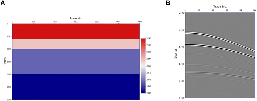
FIGURE 1. Velocity model and its forward modeling results. (A) Velocity model. (B) CMP gather.

FIGURE 2

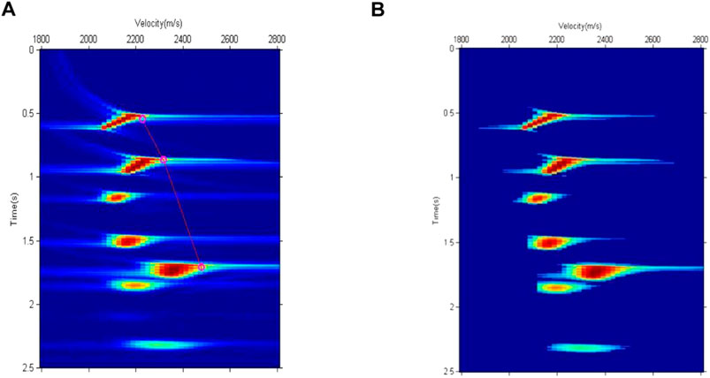
FIGURE 2. Semblance velocity spectrum and its calculation area. (A) Semblance velocity spectrum. (B) Calculation area of semblance velocity spectrum.

FIGURE 3

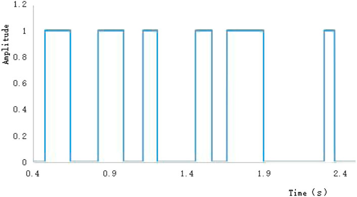
FIGURE 3. Rectangular signal.

If two energy clusters are very close in the time direction, when the number of cluster centers is calculated using the rectangular signal, the two energy clusters may correspond to the same rectangle; in other words, there may be only one cluster center. To test the velocity-picking capability in this case, the threshold of Eq. 3 was set to a small value, such that the fifth and sixth adjacent energy clusters were indistinguishable. In the rectangular signal shown in Figure 3, these two indistinguishable energy clusters correspond to only one rectangle, and each of the remaining energy clusters corresponds to a rectangle. Because these seven energy clusters have only six rectangles, the number of cluster centers in velocity picking is six. The center time of each rectangular signal was set as the initial time of each cluster center and the reference velocity corresponding to the initial time was used as the initial velocity of each cluster center to complete the calculation of its initial value. The initial values of the cluster centers are listed in Table 1. Because each initial value was calculated using the rectangular signal and reference velocity, it was relatively close to the true value and the velocity picking could be completed quickly. Owing to the poor convergence of the semblance velocity spectrum of the model data, the average amplitude velocity spectrum calculated by Eq. 10 was used to determine the velocity. The position of the velocity point culling in the average amplitude velocity spectrum was the same as that of the semblance velocity spectrum; hence, the selected area of the average amplitude velocity spectrum shown in Figure 4 was obtained. Using the initial values of the cluster centers given in Table 1 and the velocity spectrum data shown in Figure 4, the conventional k-means clustering method and the weighted k-means clustering method proposed in this paper were used for velocity picking. Table 1 shows the picking results. The picking times were not significantly different from the initial times, indicating that the rectangular signal could effectively determine the time of the cluster center. Because the initial velocities were higher than the true velocities, the picked velocities were smaller than the initial velocities and closer to the true velocities. The six cluster centers listed in Table 1 contained multiples. According to Eq. 13, the angle between them and the reference velocity was calculated, abnormal velocities (such as multiples) were automatically eliminated, and the values of the first, second, and fifth cluster centers were finally retained. The three remaining centers were all primary energy clusters, indicating that the proposed method can effectively eliminate abnormal energy clusters.

TABLE 1

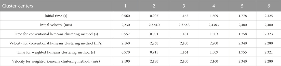
TABLE 1. Initial value and picking result of cluster centers.

FIGURE 4

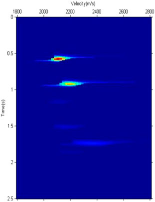
FIGURE 4. Calculation area of the average amplitude spectrum.

To test the picking accuracy of the two methods, the picking results of the conventional k-means clustering method and the weighted k-means clustering method proposed in this study are displayed in the velocity spectrum. Figure 5A shows the results of this comparison. The picked velocities of the conventional k-means clustering method are equal to or higher than those of the weighted k-means clustering method, with the picked velocities of the weighted k-means clustering method being closer to the true velocities. The conventional k-means clustering method selects the geometric centers of the velocity points involved in the calculation. If the geometric centers do not coincide with the energy cluster centers, the picking result is biased; therefore, the method is easily affected by the geometries of the energy clusters. Because the weights of the centers of the energy clusters are higher than those of other regions, the weighted k-means clustering method approaches the centers of the energy clusters in each iteration and finally yields accurate results. As shown in Figure 5A, compared with the first and second cluster centers, the velocity difference between the fifth cluster center picked up by the conventional k-means clustering method and the primary energy cluster center is smaller, owing to the influence of multiple energy clusters. However, the fifth cluster center selected by the weighted k-means clustering method is still very close to the center of the energy cluster, indicating that the method is relatively robust. For the velocity spectrum of the actual data, the energy clusters of the two primaries may be close to each other. If two primary energy clusters are treated as one cluster center, the weighted k-means algorithm selects the velocity of the stronger energy cluster. The velocity usually changes gradually from lower to greater depths. Although the velocity of the weak energy cluster cannot be determined, the velocity of the corresponding time can be obtained by interpolation.

FIGURE 5

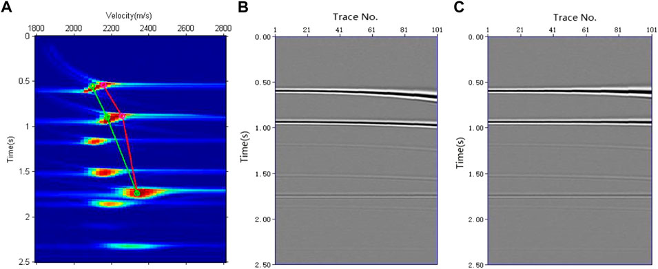
FIGURE 5. Velocity picking and normal move out (NMO) correction results. (A) Velocity picking results, where the red line is the conventional k-means clustering method and the green is the weighted k-means clustering method. (B) NMO correction results while applying velocity picked by conventional k-means clustering. (C) NMO correction results while applying velocity picked by weighted k-means clustering.

Using the time–velocity pairs picked up by these two methods, the velocities of all sampling points were obtained by interpolation. Figures 5B, C show the results of normal move out (NMO) correction using two types of velocities. Because the velocity selected by the conventional k-means clustering method was larger than the true velocity, the first, second, and fifth events in Figure 5B were insufficiently corrected. In Figure 5C, the three events are flattened, indicating that the velocity obtained by the weighted k-means clustering method was accurate. Therefore, the weighted k-means clustering method proposed in this study is superior to the conventional k-means clustering method. In terms of computational speed, the average number of iterations for the conventional k-means clustering method was seven times per CMP, whereas that for the weighted k-means clustering method was four times per CMP. Therefore, the velocity determined by the weighted k-means clustering method is fast and accurate.

Setting the threshold of Eq. 3 to a larger value can improve the discrimination ability of the adjacent energy clusters. Figure 6A shows the velocity points involved in the calculation of the semblance velocity spectrum. Compared with that in Figure 2B, the distance between the fifth and sixth energy clusters in Figure 6A is larger. Figure 6B shows the velocity points involved in the calculation of the average amplitude velocity spectrum; their positions are the same as those in Figure 6A. The rectangular signal shown in Figure 7 can be obtained using Figure 6A and the two energy clusters that cannot be distinguished in Figure 3 are shown in Figure 7. The rectangular signal in Figure 7 can determine the seven cluster centers and their initial times. The reference velocities corresponding to the initial times were used as the initial velocities of the cluster centers. Each cluster center corresponded to an energy group and their initial values are listed in Table 2. Using the initial values of the cluster centers given in Table 2 and the velocity spectrum data shown in Figure 6B, the conventional k-means clustering method and weighted k-means clustering method in this study were used for velocity picking. Table 2 presents the results. Because the conventional k-means clustering method was affected by the shape of the energy cluster, the selected velocities were greater than or equal to those of the weighted k-means clustering method. The first, second, and fifth energy clusters were retained after removing multiple energy clusters. Compared with the picking results in Table 1, the velocities of the first and second energy clusters selected by the conventional k-means clustering method in Table 2 are more accurate. The fifth energy cluster had a larger value because it was not affected by the adjacent multiple energy clusters, indicating that the conventional k-means clustering method was significantly affected by the shape of the energy clusters. The first, second, and fifth energy clusters selected by the weighted k-means clustering method in Table 2 were consistent with the velocity in Table 1, with the time values being also very close. A comparison of the results in Tables 1, 2 shows that the results obtained by the weighted k-means clustering method are more accurate than those of the conventional k-means clustering method and are not easily affected by the shapes of the energy clusters.

FIGURE 6

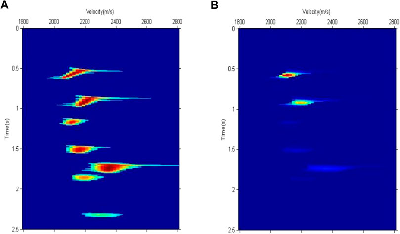
FIGURE 6. (A) Calculation area of the semblance velocity spectrum. (B) Calculation area of the average amplitude spectrum.

FIGURE 7

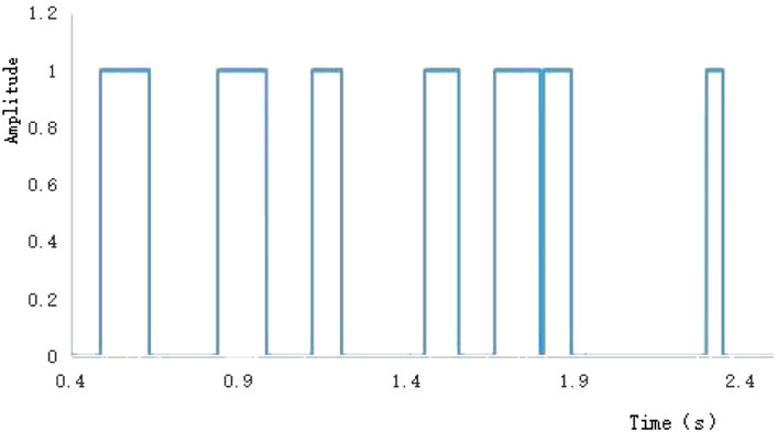
FIGURE 7. Rectangular signal.

TABLE 2

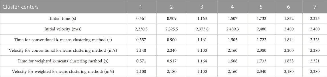
TABLE 2. Initial values and picking results for the cluster centers.

3.2 Examples of real data

The data from an actual survey line were selected to test the velocity-picking effect of the weighted k-means clustering method. The survey line contained 801 CMP gathers, the data-recording time length was 6 s, and the sampling interval was 2 ms. Due to the extremely low signal-to-noise ratio of deep seismic data, we show only the data between 0.5 and 3.0 s, based on which we analyze the velocity-picking effect. Figure 8A shows a CMP gather of the survey line, which had 240 traces in total, with a minimum offset of 360 m, and a maximum offset of 4,986 m. Figure 8B shows the semblance velocity spectrum of the CMP gather shown in Figure 8A. The seismic velocity increases from shallow to deep, and there is a certain amount of noise outside the energy cluster. The energy clusters in Figure 8B have good convergence; therefore, the semblance velocity spectrum in Figure 8B is not only used for the calculation of the number and the initial value of cluster centers, but also for the calculation of the weight of the weighted k-means clustering. Considering that there are lateral velocity changes in the actual seismic data, the velocity points within a range of 400 m from the reference velocity were used for velocity picking according to Eq. 2. The velocity-picking area is shown in Figure 9A. The velocities were picked by the conventional method and the weighted k-means clustering method proposed in this paper using the data in the picking area. To verify the accuracy of the picking results of the two methods, the time-velocity pairs picked by the conventional k-means clustering method and the weighted k-means clustering method were linearly interpolated. The interpolation results are shown in the velocity spectrum of Figure 9A for comparison. It is evident that the picking result of the conventional k-means clustering method is close to or deviates from the center of the energy cluster. The reason for this deviation is that the weights of all velocity points in the k-means clustering method are the same, and the selected cluster centers are the geometric centers of the clusters, which are easily affected by noise outside the energy clusters. Energy clusters have larger amplitudes in the central areas and smaller amplitudes in other regions. The weighted k-means clustering method can use the amplitudes to calculate the weights according to this characteristic such that the cluster centers in each iteration move quickly to the centers of the energy clusters. In the iterative process, velocity points that are far away from their cluster center are gradually eliminated to ensure that the selected velocity is the correct velocity of each energy cluster center. Figure 9B shows the NMO correction results of the velocity obtained using the conventional k-means clustering method. It is evident that the correction of the event within 1–2 s is insufficient, resulting from the high picked velocity. Figure 9C shows the NMO correction result for the velocity selected by the weighted k-means clustering method. It is evident that the event can be flattened well owing to accurate velocity picking. In terms of computational speed, the average number of iterations for the conventional k-means clustering method was 58, whereas that for the weighted k-means clustering method was five times for each CMP for velocity picking. Therefore, the weighted k-means clustering method not only has the advantage of accurate velocity picking, but also the advantage of higher computational efficiency.

FIGURE 8

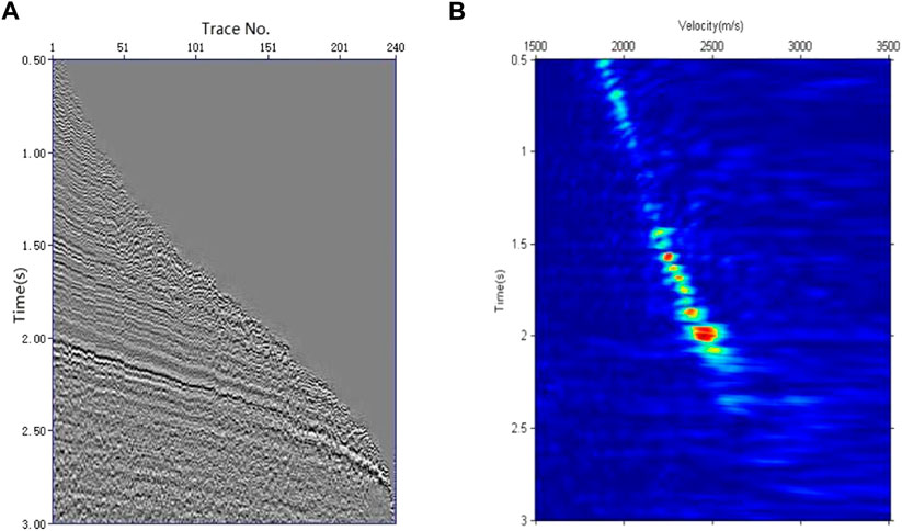
FIGURE 8. (A) CMP gather of actual data and (B) its semblance velocity spectrum.

FIGURE 9

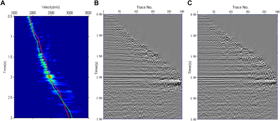
FIGURE 9. Velocity picking and NMO correction results. (A) Velocity picking results, where the red line is the conventional k-means clustering method and the green is the weighted k-means clustering method. (B) NMO correction results while applying velocity picked by conventional k-means clustering. (C) NMO correction results while applying velocity picked by weighted k-means clustering.

Figure 10A shows the manually selected velocity field. Owing to the large picking workload, the seismic velocity-picking interval was 20 CMPs and the seismic velocities of the remaining traces were obtained using the interpolation method. Because the intelligent method can determine the velocity of each CMP, its velocity field is finer than that of manual picking. To eliminate the influence of noise and other factors, the selected velocity field was smoothed in both the spatial and temporal directions. Figure 10B shows the velocity field selected by the conventional k-means clustering method; its continuity in the lateral direction was poor, and there were high-velocity outliers between 0.5 and 2.0 s. Figure 10C shows the velocity field selected by the weighted k-means clustering method, which is roughly consistent with the manually selected velocity field shown in Figure 10A.

FIGURE 10

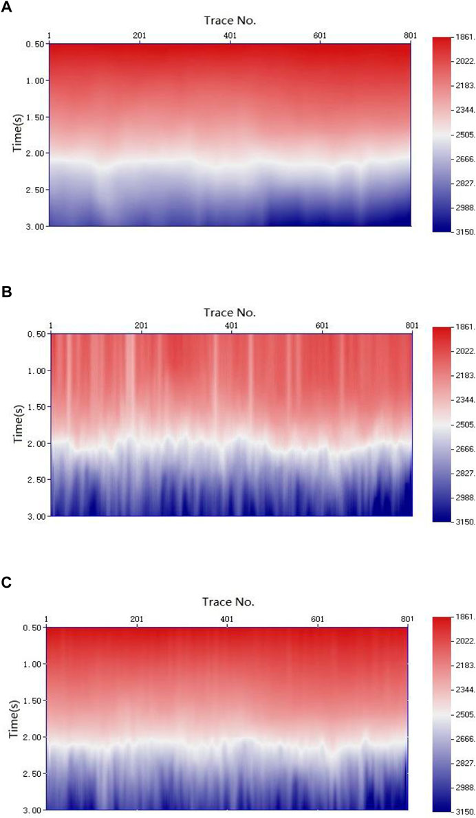
FIGURE 10. (A) Velocity field picked by the manual method. (B) Velocity field picked by the conventional k-means clustering method. (C) Velocity field picked by weighted k-means clustering method.

To verify the correctness of the velocity picking, the CMP gathers were NMO corrected using the three types of velocity fields in Figure 10. The stacked profiles were subsequently obtained by stacking. Owing to the inaccuracy of the velocities, the stacked profile (Figure 11B) obtained by applying the velocities selected by the conventional k-means clustering method showed discontinuities. The stacked profile obtained with the velocities selected by the weighted k-means clustering method (Figure 11C) was very close to that obtained by applying the manually selected velocities (Figure 11A), indicating that the velocities selected by the weighted k-means clustering method were accurate. Figure 12 shows the result of magnifying the anticlinal parts of Figures 11A, C. Figures 12A, B have almost the same structure in the box, but the energy of the events in Figure 12B is stronger, indicating that the velocity picked by the weighted k-means clustering method was more accurate than that picked manually. A more precise reason is that the weighted k-means clustering method can determine the velocity of each CMP, whereas the manual method usually selects the velocity at a certain CMP interval.

FIGURE 11

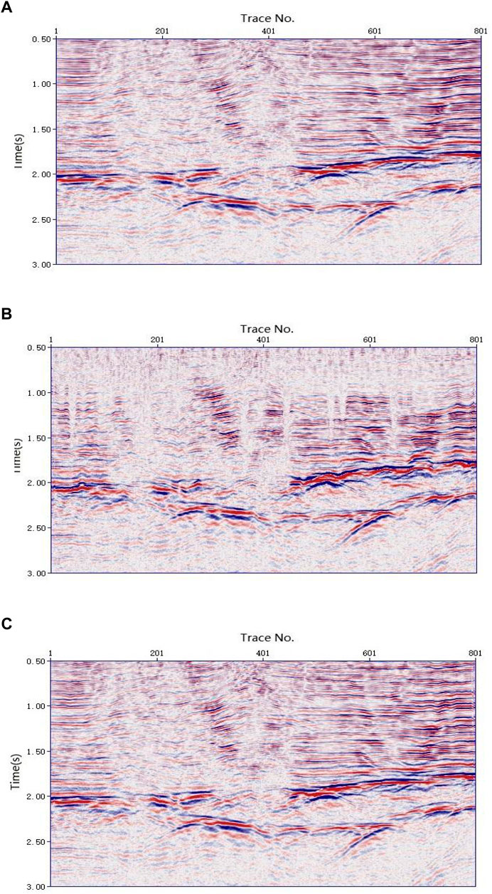
FIGURE 11. Stacked profiles obtained by applying three kinds of velocity fields. (A) Stacked profile obtained by applying the manually picked velocities. (B) Stacked profile obtained by applying the velocities picked by the conventional k-means clustering method. (C) Stacked profile obtained by applying the velocities picked by the weighted k-means clustering method.

FIGURE 12

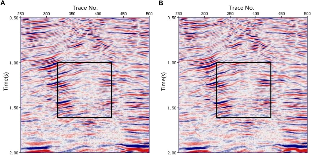
FIGURE 12. Enlarged display of the anticline. (A) Stacked profile obtained by applying the manually picked velocities. (B) Stacked profile obtained by applying the velocities picked by the weighted k-means clustering method.

4 Conclusion

In the velocity spectrum, the amplitude is large at the center of the energy cluster and small in other regions. Based on this feature, this study proposes an unsupervised weighted k-means clustering intelligent velocity-picking method based on prior information constraints. Through processing of model and real data, we prove that the method is effective and feasible and conclude the following.

Under the constraint of the reference velocity, we can not only delineate the picking area and reduce the velocity points involved in the calculation but also use the reference velocity as the initial velocity of the cluster center. In the velocity spectrum, there were many velocity points with larger amplitudes near the center of the primary energy cluster. According to this feature, the number of cluster centers and the initial time of each cluster center could be obtained by counting the number of velocity points with larger amplitudes corresponding to each time-sampling point.

Owing to the effect of the weights, in the iterative weighted k-means clustering method, the distance between the cluster center and the energy cluster center is very close. Some of the velocity points far from the cluster center can be gradually eliminated, which speeds up the calculation and reduces the interference of noise, so that the cluster center moves quickly to the center of the energy cluster. Therefore, compared with the conventional k-means clustering method, the seismic velocity-picking method of weighted k-means clustering proposed in this paper is not only fast in calculation, but also more accurate in picking results.

The method proposed here can only adapt to the velocity spectrum with a relatively high signal-to-noise ratio. For a velocity spectrum with a very low signal-to-noise ratio, it may not be possible to accurately determine the velocity. The proposed method is limited by the accuracy of the velocity spectrum to a certain extent. If the velocity interval of the velocity spectrum is too large, the picking accuracy is low. If the amplitude of the weakly reflected energy cluster is lower than the amplitude threshold $thre1$ in Eq. 3, the proposed method cannot determine its velocity.

Data availability statement

The datasets presented in this article are not readily available because the data are confidential. Requests to access the datasets should be directed to JX, xiejunfa@petrochina.com.cn.

Author contributions

JX contributed to the conceptualization, writing (original draft), writing (review and editing), programming, and methodology. XX contributed to writing, reviewing, editing, and methodology. YL contributed to the data processing and writing, review, and editing. XS contributed to the writing, reviewing, and editing of the manuscript. YY contributed to conceptualization, writing, reviewing, editing, supervision, project administration, and funding acquisition. DW contributed to the conceptualization and programming.

Funding

This research was funded by the Research on Reservoir-forming theory and exploration technology of marine carbonate rocks (2021DJ0506) and estimation of near-surface velocity and Q value using seismic surface wave characteristics (2022KT1503) provided by Petrochina.

Conflict of interest

The authors JX, XX, XS, YY and DW were employed by the Northwest Branch of Research Institute of Petroleum Exploration and Development, PetroChina.

The author YL was employed by the Xinjiang Oilfield Company, PetroChina.

Publisher’s note

All claims expressed in this article are solely those of the authors and do not necessarily represent those of their affiliated organizations, or those of the publisher, the editors and the reviewers. Any product that may be evaluated in this article, or claim that may be made by its manufacturer, is not guaranteed or endorsed by the publisher.

References

Almarzoug, A. M., and Ahmed, F. Y. (2012). “Automatic seismic velocity picking,” in 2012 SEG Annual Meeting, Las Vegas, Nevada, November 4-9 2012. doi:10.1190/segam2012-0294.1

CrossRef Full Text | Google Scholar

Biswas, R., Vassiliou, A., Stromberg, R., and Sen, M. K. (2018). “Stacking velocity estimation using recurrent neural network,” in 2018 SEG International Exposition and Annual Meeting, Anaheim, California, USA, October 2018. doi:10.1190/segam2018-2997208.1

CrossRef Full Text | Google Scholar

Chen, Y. (2018). Automatic microseismic event picking via unsupervised machine learning. Geophys. J. Int. 212, 1750–1764. doi:10.1093/gji/ggaa186

CrossRef Full Text | Google Scholar

Chen, Y. (2018). “Automatic semblance picking by a bottom-up clustering method,” in SEG 2018 Workshop: SEG Maximizing Asset Value Through Artificial Intelligence and Machine Learning, Beijing, China, 17-19 September 2018. doi:10.1190/AIML2018-12.1

CrossRef Full Text | Google Scholar

Choi, H., Byun, J., and Seol, S. J. (2010). Automatic velocity analysis using bootstrapped differential semblance and global search methods. Explor. Geophys. 63, 31–39. doi:10.1071/EG10004

CrossRef Full Text | Google Scholar

Dong, L. P., and He, X. (1996). Automatic velocity pickup with artificial neural network. Oil Geophys. Pet. 31, 98–103. (In Chinese)CNKI:SUN:SYDQ.0.1996-S1-015.

Google Scholar

Fabien-Ouellet, G., and Sarkar, R. (2020). Seismic velocity estimation: A deep recurrent neural-network approach. Geophysics 85, U21–U29. doi:10.1190/geo2018-0786.1

CrossRef Full Text | Google Scholar

Fish, B. C., and Kusuma, T. (1994). “A neural network approach to automate velocity picking,” in 1994 SEG Annual Meeting, Los Angeles, California, October 23-28 1994. doi:10.1190/1.1822888

CrossRef Full Text | Google Scholar

Fomel, S. (2009). Velocity analysis using AB semblance. Geophys. Prospect. 57, 311–321. doi:10.1111/j.1365-2478.2008.00741.x

CrossRef Full Text | Google Scholar

Grigorios, T., and Aristidis, L. (2014). The MinMax K-means clustering algorithm. Pattern Recognit. 47, 2505–2516. doi:10.1016/j.patcog.2014.01.015

CrossRef Full Text | Google Scholar

Kumar, K. M., and Reddy, A. R. M. (2017). An efficient K-means clustering filtering algorithm using density based initial cluster centers. Inf. Sci. 418, 286–301. doi:10.1016/j.ins.2017.07.036

CrossRef Full Text | Google Scholar

Lumley, D. E. (1997). Monte Carlo automatic velocity picks. Stanf. Explor. Proj. 75, 1–25.

Google Scholar

Ma, Y., Ji, X., Fei, T. W., and Luo, Y. (2018). “Automatic velocity picking with convolutional neural networks,” in 2018 SEG International Exposition and Annual Meeting, California, USA, October 14-19 2018. doi:10.1190/segam2018-2987088.1

CrossRef Full Text | Google Scholar

Marco, C., Aritz, P., and Jose, A. L. (2017). An efficient approximation to the K-means clustering for massive data. Knowledge-Based Syst. 117, 56–69. doi:10.1016/j.knosys.2016.06.031

CrossRef Full Text | Google Scholar

Neidell, N. S., and Taner, M. T. (1971). Semblance and other coherency Measures for multichannel data. Geophysics 36, 482–497. doi:10.1190/1.1440186

CrossRef Full Text | Google Scholar

Park, M. J., and Sacchi, M. (2020). Automatic velocity analysis using convolutional neural network and transfer learning. Geophysics 85, V33–V43. doi:10.1190/geo2018-0870.1

CrossRef Full Text | Google Scholar

Schmidt, J. (1992). “Neural network stacking velocity picking,” in 1992 SEG Annual Meeting, New Orleans, Louisiana, October 25-29 1992. doi:10.1190/1.1822036

CrossRef Full Text | Google Scholar

Smith, k. (2017). “Machine learning assisted velocity autopicking,” in 2017 SEG International Exposition and Annual Meeting, Houston, Texas, September 24–29, 2017. doi:10.1190/segam2017-17684719.1

CrossRef Full Text | Google Scholar

Thierry, C., Manuel, P., and Kostia, A. (2003). Unsupervised seismic facies classification:A review and comparison of techniques and implementation. Lead. Edge 22, 942–953. doi:10.1190/1.1623635

CrossRef Full Text | Google Scholar

Toldi, J. L. (1989). Velocity analysis without picking. Geophysics 54, 191–199. doi:10.1190/1.1442643

CrossRef Full Text | Google Scholar

Wang, D., Yuan, S. Y., Yuan, H., Zeng, H. H., and Wang, S. X. (2021). Intelligent velocity picking based on unsupervised clustering with the adaptive threshold constraint. Chin. J. Geophys 64, 1048–1060. (In Chinese). doi:10.6038/cjg2021O0305

CrossRef Full Text | Google Scholar

Wei, S., Yonglin, O., Qingcai, Z., and Yaying, S. (2018). “Unsupervised machine learning: K-Means clustering velocity semblance auto-picking.” in 80th EAGE Conference and Exhibition, Copenhagen, Denmark, June 11-14, 2018, doi:10.3997/2214-4609.201800919

CrossRef Full Text | Google Scholar

Xie, J. F., Sun, C. Y., Wang, X. M., Li, H. M., and Lin, M. Y. (2017). The multi-criteria velocity analysis of seismic data. Geophys. Geochem. Explor. 41, 513–520. (In Chinese). doi:10.11720/wtyht.2017.3.17

CrossRef Full Text | Google Scholar

Yuan, S. Y., Jiao, X. Q., Luo, Y. N., Sang, W. J., and Wang, S. X. (2022). Double-scale supervised inversion with a data-driven forward model for low-frequency impedance recovery. Geophysics 87, R165–R181. doi:10.1190/geo2020-0421.1

CrossRef Full Text | Google Scholar

Zha, C. Y. (1996). Stack velocity pickup using neural network. Oil Geophys. Pet. 31, 892–897. (In Chinese)CNKI:SUN:SYDQ.0.1996-06-018.

Google Scholar

Zhang, L. (1997). Automatic picking and its applications. Standford Explor. Proj. 70, 280–299.

Google Scholar

Zhang, L., and Claerbout, J. (1998). Automatic dip-picking by non-linear optimization. Standford Explor. Proj. 67, 123–138.

Google Scholar

Zhang, L., Zhu, P. M., Gu, Y., and Li, X. (2019). “Automatic velocity picking based on deep learning,” in SEG International Exposition and Annual Meeting, San Antonio, Texas, USA, September 15-20 2019. doi:10.1190/segam2019-3215633.1

CrossRef Full Text | Google Scholar

Zhang, P., and Lu, W. (2016). Automatic time-domain velocity estimation based on an accelerated clustering method. Geophysics 81, U13–U23. doi:10.1190/geo2015-0313.1

CrossRef Full Text | Google Scholar

Zhou, Z. S., Zeng, W. Z., Liu, S. Q., and Chen, W. X. (2020). First arrival picking method by seismic multi-attribute based on weighted K-means clustering algorithm. Acta Seismol. Sin. 42, 177–186. (In Chinese). doi:10.11939/jass.20190107

CrossRef Full Text | Google Scholar