 Ziduo Hu
 Jidong Yang
 Linghe Han1
 Jianping Huang
 Youcai Yu
- 1Research Institute of Petroleum Exploration and Development-Northwest PetroChina, Lanzhou, China
- 2School of Geosciences, Laboratory for Marine Mineral Resources, National Laboratory for Marine Science and Technology, China University of Petroleum (East China), Qingdao, Shandong, China
The thick Quaternary loess on the Loess Plateau of China produces strong seismic attenuation, resulting in weak reflections from subsurface exploration targets. Accurately simulating seismic wavefield in the Loess Plateau is important for guiding subsequent data processing and interpretation. We present a 2D/3D wavefield simulation method for the Loess Plateau using a viscoacoustic wave equation with explicitly expressed quality factor. To take into account the effect of irregular surface, we utilize a vertically deformed grid to represent the topography, and solve the viscoacoustic wave equation in a regular computational domain that conforms to topographic surface. Grid deformation introduces the partial derivatives such as ∂vx/∂z and ∂vy/∂z in the wave equation, which is difficult to be accurately computed using traditional staggered-grid finite-difference method. To mitigate this issue, a finite-difference scheme based on a fully staggered-grid is adopted to solve the viscoacoustic wave equation. Numerical experiments for a simple layer model and 2D/3D realistic Loess Plateau models demonstrate the feasibility and adaptability of the proposed method. The 3D modeling results show comparable amplitude and waveform characteristics to the field data acquired from the Chinese Loess Plateau, suggesting a good performance of the proposed modeling method.
Introduction
Seismic modeling always plays an important role in the study of wave phenomenon, and provides numerical propagators for seismic imaging and inversion (Bording and Lines, 1997; Virieux et al., 2009). According to theoretical background and numerical implementation, seismic modeling approaches can be categorized into two basic groups (Carcione et al., 2002): ray-based and wave-equation methods. Each group has its own pros and cons, and both of them have been widely used in seismic modeling, imaging and inversion.
Seismic ray is a high-frequency asymptotic solution of the wave equation (Červený, 2001), of which the traveltime and amplitude are determined by the eikonal and transport equations, respectively. It decomposes the coupled wavefields into independent single-phase waves, including direct wave, reflection, refraction, transmission, converted wave, multiples, etc (Červený et al., 2007). This makes it easy to study a specific wave phenomenon in complicated subsurface structures. In the past half century, ray-based methods have evolved from classical kinematic ray tracing (Julian and Gubbins, 1977; Um and Thurber, 1987), through paraxial ray tracing (Beydoun and Keho, 1987) and Maslov asymptotic theory (Maslov et al., 1972; Chapman and Drummond, 1982; Kendall and Thomson, 1993), then to Gaussian beam (Červený et al., 1982; Müller, 1984; Nowack and Aki, 1984). Due to high computational efficiency, ray-based Kirchhoff and beam migrations have become routine tools for seismic imaging and migration velocity analysis in the industry (Hill, 1990, 2001; Gray and May 1994; Yang et al., 2018, 2022).
The other group of seismic modeling is to directly solve the wave equation onto a discretized grid using numerical solvers. Typical numerical algorithms include finite-difference, finite-element, pseudo-spectrum, spectrum-element and boundary-element approaches (Carcione et al., 2002). Because of relatively cheap cost, the finite-difference has been extensively used for wavefield simulation (Kristek and Moczo, 2003; Etgen and O’Brien, 2007), reverse-time migration (McMechan, 1989; Wu et al., 1996) and full-waveform inversion (Mulder and Plessix, 2008; Vigh et al., 2009; Virieux and Operto, 2009) in exploration seismology. Using the triangle or tetrahedral mesh to discretize the geological model, the finite-element approach can accurately simulate wave propagation in strong heterogeneous media (Marfurt, 1984; De Basabe and Sen, 2009; Komatitsch et al., 2010). But due to large computational cost, it is usually limited for small-scale problems, e.g., in the fault zone and oil & gas reservoir. The spectrum-element method inherits the flexibility of finite-element and the accuracy of spectral method, and the diagonal mass matrix using a specific discretization and integration rule results in a higher efficiency than finite-element method (Komatitsch and Tromp, 1999; Komatitsch et al., 2000; Komatitsch and Tromp, 2002). These advantages make it have be widely applied to wavefield simulation and adjoint tomography in regional and global seismology (Komatitsch et al., 2002; Tape et al., 2009; Lei et al., 2020).
The Loess Plateau of China has the thickest and largest loess coverage in the world, which was deposited in the Pleistocene under particular geological, geomorphological and climatic conditions (Sun, 2002). Rich oil and gas resource under the loess promote extensive seismic exploration in this area. Low-velocity loess layer and complicated topography produce strong seismic attenuation and scattering noise, resulting in deep reflections with a very low signal-to-noise ratio (SNR). The low-quality observed data present a large challenge for subsequent processing and interpretation (Wang et al., 2004; Wang et al., 2014). Accurately simulating the wavefields of the Loess Plateau helps to understand noise generation mechanism and attenuation effect of thick loess layer, which can guide subsequent data processing and imaging. In the wavefield modeling for the Loess Plateau, it is necessary to take into account the irregular topography and strong attenuation due to complex near-surface geology.
There are many rheological models to characterize seismic attenuation during wave propagation. For instance, a complex-valued velocity can be directly introduced into the frequency-domain wave equation to describe phase dispersion and amplitude dissipation (Liao and McMechan, 1996; Stekl and Pratt, 1998; Aki and Richards, 2002). On the other hand, in the time domain, the nearly constant attenuation effect within a frequency band can be implemented by a combination of springs and dashpots in series and/or parallel (Carcione, 2007). Typical viscous models include classical and generalized Maxwell body (Emmerich and Korn, 1987), Kelvin-Voigt body (Carcione et al., 2004), and standard linear solid body (Liu et al., 1976; Carcione, 1993; Guo et al., 2019). Using a fractional time derivative, Kjartansson (1979) presented an alternative constant quality factor (Q) model to describe the stress and strain relation. Zhu and Harris (2014) utilized a fractional Laplacian operator to approximate the fractional time derivative and obtained a simplified constant-Q wave equation. Later, many hybrid-domain solvers, including local homogeneous approximation (Chen et al., 2016; Wang et al., 2017; Xing and Zhu, 2019; Wang et al., 2022), low-rank approximation (Sun et al., 2015), Hermite distributed approximation (Yao et al., 2017), are proposed to produce more accurate numerically solution. Recently, Yang and Zhu (2018) presented a complex-valued wave equation to simulate viscoacoustic wave propagation, which has an explicitly expressed Q and can be easily used in full-waveform inversion (Yang et al., 2020).
The Loess Plateau of China has diverse geomorphic features, such as hill, tableland, ditch, ridges and mounds, which results into a complex irregular topography. In seismic modeling using the finite-difference, many strategies have been developed to handle topography and free surface. Levander (1988) implemented a flat free-surface boundary condition using the image method. Later, this approach was extended to highly irregular topography by Robertsson (1996). Mittet (2002) treated elastic Hooke’s tensor on the free surface as that in a transversely isotropic medium and presented a simple implementation of free-surface. Nakamura et al. (2012) proposed an efficient Heterogeneity, Oceanic layer and Topography (HOT) finite-difference method to compute wavefields at the solid-air, fluid-air and fluid-solid boundaries. Instead of directly representing the topography at a regularly and densely sampled Cartesian grid, an alternative way is to transform the physical curved domain to a regular computational grid (Hestholm and Ruud, 1994; Hestholm and Ruud, 1998). This curvilinear transformation can avoid the strong scatterings from the staircase topography and is relatively easily to implement the free-surface condition (Hestholm, 1999; Hestholm and Ruud, 2002; Zhang et al., 2012). At current stage, this approach has been extended to conform both topographic surface and interior layers in viscous and anisotropic media (Sun et al., 2016; Shragge and Tapley, 2017; Konuk and Shragge, 2020; Sun et al., 2021).
In this work, we present a viscoacoustic modeling method to study seismic wave phenomena in the Loess Plateau. A viscoacoustic wave equation is first derived based on a non-linear optimization for the frequency-independent Q effect within a frequency band (Fichtner and van Driel, 2014). To conform to the topographic surface, a vertically deformed grid is adopted to transform the irregular domain to a regular computational coordinate (Jastram and Tessmer, 1994; de la Puente et al., 2014). This strategy does not introduce as many additional partial derivatives as the curvilinear grid method that deforms along three axises, and thus it does not increase too much computational cost compared with that computed on traditional Cartesian grid. In addition, to accurately compute the spatial derivatives such as ∂vx/∂z and ∂vy/∂z, we apply a fully staggered-grid finite-difference scheme (Lisitsa and Vishnevskiy, 2010; de la Puente et al., 2014) to numerically solve the viscoacoustic wave equation on a vertical deformed grid. Numerical experiments for a simple layer model and 2D/3D Loess Plateau models as well as a comparison between synthetic and field data demonstrate the proposed method can accurately simulate wave propagation in the Loess Plateau with thick loess layers.
Theory
Viscoacoustic wave equation with explicitly expressed Q
In viscoacoustic medium, the pressure p (x, t) and particle velocity v (x, t) satisfy a constitutive relation as
where v = (vx, vy, vz), and subscripts x, y and z denote particle velocity components along different axises. κ(x, t) is a time-dependent bulk modulus and can be constructed by superposing N groups of relaxation mechanisms (Fichtner and van Driel, 2014):
where
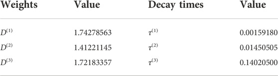
TABLE 1. The weights and decay times of three relaxation mechanisms used in the viscoacoustic modeling.
Taking the time derivative of κ(x, t), we have
where δ(t) is the Kronecker delta function, and s is the summation of weights, i.e.,
where the memory variables Φ(l)(x, t) are defined as
and satisfy
Considering the second Newton law and assembling Eqs 4, 6, we obtain a viscoacoustic wave equation with the explicitly expressed Q as
where xs denotes the source location, and f(t) is the source time function.
Compared with existing viscoacoustic wave equations, such as the standard linear solid model (Carcione, 1990; Guo and Mcmechan, 2017) and fractional-Laplacian method (Zhu and Harris, 2014; Xing and Zhu, 2019), Eq. 7 has the following advantages in seismic modeling. 1) The quality factor Q is explicitly incorporated in the wave equation, which does not need to be converted to stress and strain relaxation times as in the standard linear solid method. 2) Eq. 7 can be efficiently solved using any time-domain finite-difference schemes, which does involves the Fourier transform or more complicated mixed-domain solvers as in the fractional Laplacian based methods. 3) As shown in Fichtner and van Driel (2014), the frequency-dependent Q effect can also be simulated by recomputing the weights D(l) and relaxation times τ(l).
Representation of the topographic surface on vertically deformed grids
To conform to the topographic surface of the Loess Plateau, here we use a vertically deformed grid to map the irregular physical space x = (x, y, z) to a regular computational domain α = (α, β, γ), which is given by
where ζ(x, y) is the elevation of topography (Figure 1), zmax is the maximum depth of the region of interest, γmax = zmax+ζmax, and ζmax is the maximum of elevation.
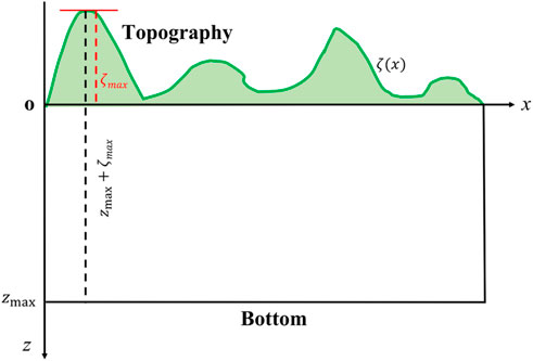
FIGURE 1. An example of 2D topography to illustrate the basic parameters in the mapping from the physical space to computational domain.
With the coordinate transform relation in Eq. 8, the partial derivatives can be computed as
By setting
The viscoacoustic wave equation in Eq. 7 can be rewritten in the new coordinate as
With a generalized partial derivative operator
The proposed viscoacoustic wavefield simulation in a vertical stretched grid can be summarized into the following steps. First, with the elevation of topography ζ(x, y), we compute its derivative with respect to x and y and the topography related coordinate stretching parameters cx and cy. Then, the irregular physical space is mapped to a regular computational domain by vertical stretching according to Eq. 8, in which velocity, density and Q parameters onto the computational grids are calculated using a linear interpolation method. Next, the viscoacoustic wave equation 11 is solved in a regularly-sampled computational domain using any available numerical solvers. Finally, the wavefields in the real physical space are reconstructed by mapping the extrapolated wavefields back with the same interpolation algorithm used in the second step.
Numerical implementation using a fully staggered-grid finite difference scheme
Considering the trade-off of computational accuracy and efficiency, we choose the time-domain staggered-grid finite-difference scheme to solve the viscoacoustic wave Eq. 11. Because of vertical stretching, it is difficult for the standard staggered-grid finite-difference method (Virieux, 1986) to accurately compute the partial derivatives such as ∂vx/∂γ and ∂vy/∂γ. Here we discretize and solve the wave equation using a fully staggered-grid approach (Lebedev, 1964; Lisitsa and Vishnevskiy, 2010; de la Puente et al., 2014). The nodes distribution is presented in Figure 2. Unlike the standard staggered-grid approach, the fully staggered-grid finite-difference scheme has three particle velocity components at the half grids (yellow triangles in Figure 2B), and three additional pressure wavefields (red circles in Figure 2B). For the time derivative, we still adopt a second-order finite-difference method, which results in the following updating scheme:
where Di (i = α, β, γ) denotes the finite-difference operator for first-order spatial derivative. All components of pressure, particle velocity and memory variable wavefields are iteratively computed based on Eq. 13, and each partial derivative can be accurately calculated. Taking pn+1 at (i, j, k) as an example, we compute
where c is the summation of finite-difference coefficients, vmax denotes the maximum velocity, Qmin denotes the minimum quality factor value, and
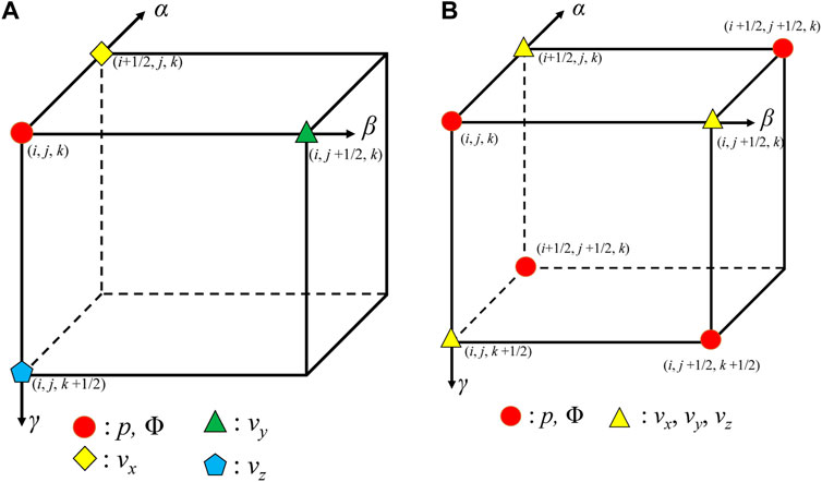
FIGURE 2. Comparison of the node distribution in the standard (A) and fully (B) staggered-grid finite-difference methods. p denotes the pressure wavefield, Φ denotes the memory variable, and
The free-surface boundary condition in the viscoacoustic modeling is implemented using a simple image method (Zhang et al., 2012). In addition, because two types of grids at different locations are coupled in the fully staggered-grid finite-difference scheme, spurious waves may occur if loading source incorrectly (Koene et al., 2021). To avoid these spurious waves, we adopt the strategy proposed by Lisitsa and Vishnevskiy (2010) and de la Puente et al. (2014), which is implemented for loading a point source by adding the source function at a node of (i, j, k) and at additional sub-nodes of (i ± 1/2, j ± 1/2, k) (i ± 1/2, j, k ± 1/2), (i, j ± 1/2, k ± 1/2) with a scale of 0.25. Seismograms are extracted using a similar strategy by summing the weighted records at a main node and sub-nodes of receiver locations.
A simulation example for a homogeneous model is presented in Figure 3. P-wave velocity is 3 km/s, Q is 50, and a 200-m-thick vacuum layer is set at the top to simulate surface reflections. Acoustic and two kinds of viscoacoustic solvers are used to compute seismic wavefields, and the result of generalized standard linear solid (GSLS) method is used as a reference for comparison. Because of the phase dispersion and energy dissipation, viscoacoustic waves propagate faster than acoustic waves and have much weaker amplitudes (Figures 3C,D). The surface at the z = 0 km produces a reflection with opposite polarity compared with the direct wave (Figure 3B). The waveforms computed using the proposed method have good agreements with those of GSLS in terms of both phases and amplitudes (red dot and black solid lines Figures 3C,D).
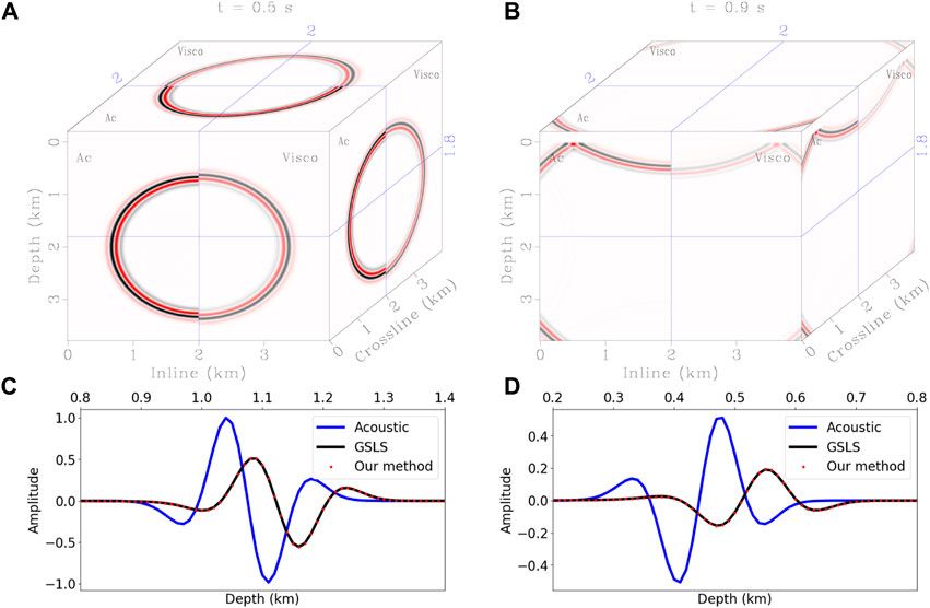
FIGURE 3. Comparison of wavefield simulation in a homogeneous medium. Panels (A,B) are acoustic (Ac) and viscoacoustic (Visco) wavefields at 0.5 s and 0.9 s. Panels (C,D) are single-trace comparisons extracted from (A,B). Blue solid lines denote acoustic results. Black solid lines denote viscoacoustic results computed using the generalized standard linear solid (GSLS) method, which are used as the references. Red dot lines are the results computed using the proposed method.
Numerical experiments
To test the performance of the proposed viscoacoustic modeling method, we apply it to a simple layer model and 2D/3D realistic Loess Plateau models. In the computation, the spatial accuracy of finite-difference is eighth order and the temporal accuracy is second order.
A simple layer model
The first example is a three layer model, of which the velocity and Q values are shown in Figure 4A. A sinusoidal topography is designed to simulate the irregular surface. This model is discretized on a 601 × 501 grid with a 10-m spatial increment. A Ricker wavelet with the peak frequency of 15 Hz is used as the source time function. The source is deployed 10 m below the topography, and 501 receivers are evenly distributed horizontally on the observation surface. Time increment is 1 ms and duration is 6 s. Figure 4B shows the vertically distorted model in the computational domain. The topography has been fattened, but the originally horizontal interfaces in subsurface are curved. This coordinate conversion make it easy to simulate wave propagation in the near surface region.

FIGURE 4. A three-layer model in the physical space (A) and computational domain (B). Red star denotes the source location, and magenta line denotes receivers.
The snapshots computed by solving the viscoacoustic and acoustic wave equations with and without the free surface are presented in Figures 5, 6. In the computational domain, the wavefronts of direct and reflected waves are distorted because of cx, cy, and cz coefficients in Eq. 11 associated with the topography (Figure 5A–C, Figure 6A–C). In contrast, in the physical domain, the direct wave becomes regular with a half-circle wavefront, and transmitted and reflected waves are generated at the interfaces (Figure 5D–F, Figure 6D–F). The free surface at topography produces complicated boundary reflections, which intersects with deep effective wavefields (Figures 6D–F). Compared with acoustic modeling results, viscoacoustic wavefields have similar amplitudes and phases during early time, but they show considerably traveltime and amplitude differences as the propagation time increases (Figure 7).
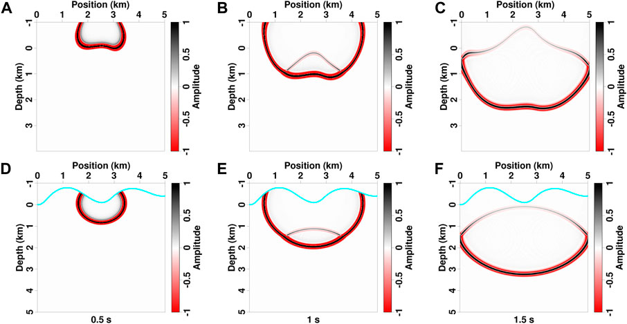
FIGURE 5. Viscoacoustic wavefields of different propagation times with a top absorption boundary in the computational domain (A–C) and physical space (D–F). The cyan lines in panels (D–F) denote the topography.
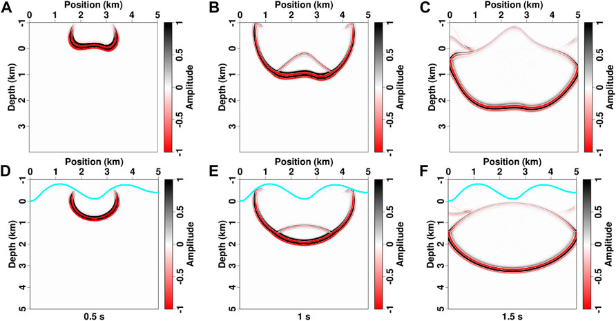
FIGURE 6. Viscoacoustic wavefields of different propagation times with a free-surface boundary in the computational domain (A–C) and physical space (D–F). The cyan lines in panels (D–F) denote the topography.
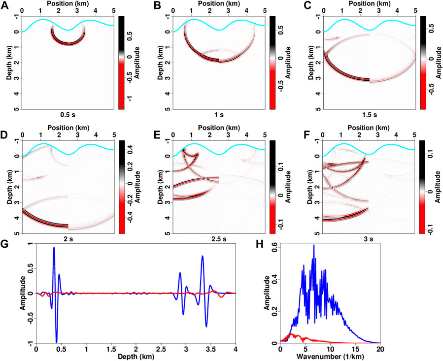
FIGURE 7. (A–F) Comparisons of acoustic (left half panel) and viscoacoustic (right half panel) wavefields at different propagation times. A free surface is used as the boundary condition on the topography. (G) Single-trace comparison at x = 3 km, and (H) corresponding spectra comparison, in which blue lines denotes acoustic results and red lines denote viscoacoustic results. The cyan lines in (A–F) denote the topography.
The common-shot gathers are presented in Figures 8, 9. For comparison, we also compute the record using the GSLS method and utilize it as a reference, in which three relaxation mechanisms are used to approximate a frequency-independent Q. Without the free surface, common-shot records only have a direct wave and two subsurface reflections. The direct waves computed using acoustic and viscoacoustic simulations have similar waveforms due to short propagation time. By contrast, the deep reflectors of viscoacoustic records, especially for the one from second interface, have different phases and much weaker amplitudes than acoustic records (Figure 8D). The GSLS benchmark result has a good agreement with that of the proposed method, indicating that the new method can accurately simulate viscoacoustic propagation with irregular topography (black solid lines and red dot lines in Figures 8D, 9D). In addition, the reflected events are no longer hyperbolic due to topographic surface, and incorporating the free surface in the modeling introduces many surface-related multiples (Figure 9).
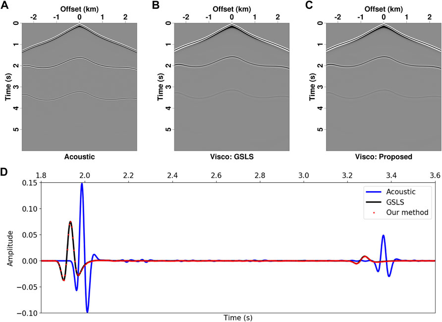
FIGURE 8. Common-shot gathers simulated with a top absorption boundary for the three-layer model. (A) Acoustic modeling, (B) viscoacoustic modeling using the GSLS method, (C) viscoacoustic modeling using the proposed method, and (D) single-trace comparison at the offset of −2.3 km. The amplitudes of panel (D) are normalized by the maximum value of direct waves.
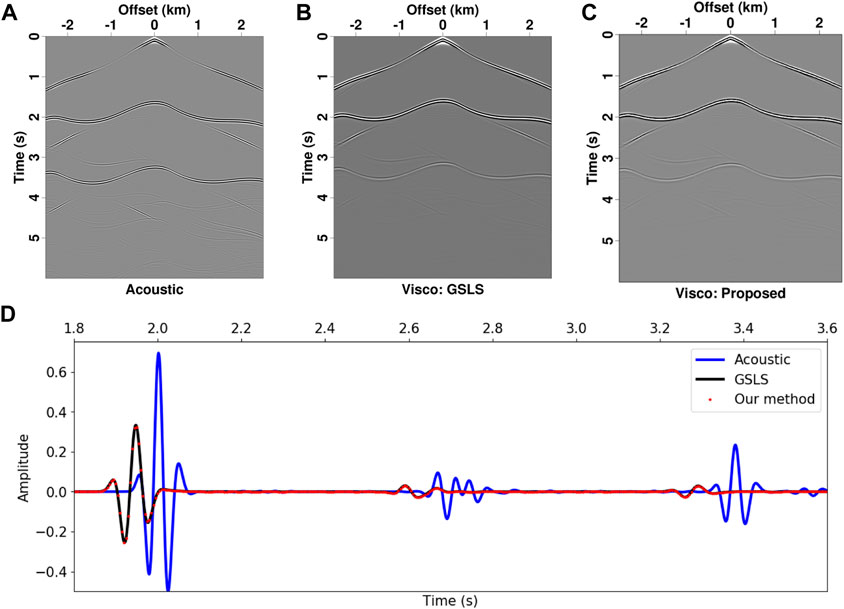
FIGURE 9. (A–D) Common-shot gathers simulated with a top free-surface boundary for the three-layer model. The panel notifications are the same as in Figure 8.
2D Loess Plateau model
According to the outcrop of Chinese Loess Plateau, we build a realistic model for seismic modeling (Figure 10). Four layers are designed to mimic real loess structures: 1) a weathering layer with dry loess, 2) a low-velocity layer with wet loess, 3) a transition layer with water saturated loess, and 4) a Tertiary soil layer. Detailed P-wave velocity and Q values of these layers are given in Table 2. The maximum thickness of loess is about 300 m (Figure 10A), and low Q values in the dry and wet loess layers can produce strong seismic attenuation. This model is discretized onto a 1,000 × 2601 grid with a 5-m spacing. The source is located at x = 6.15 km horizontally and z = −1.18 km vertically with a 15-Hz Ricker wavelet as the source time function. The projected velocity in the computational domain is shown in Figure 10B, of which the surface is flattened and subsurface structures are slightly distorted.
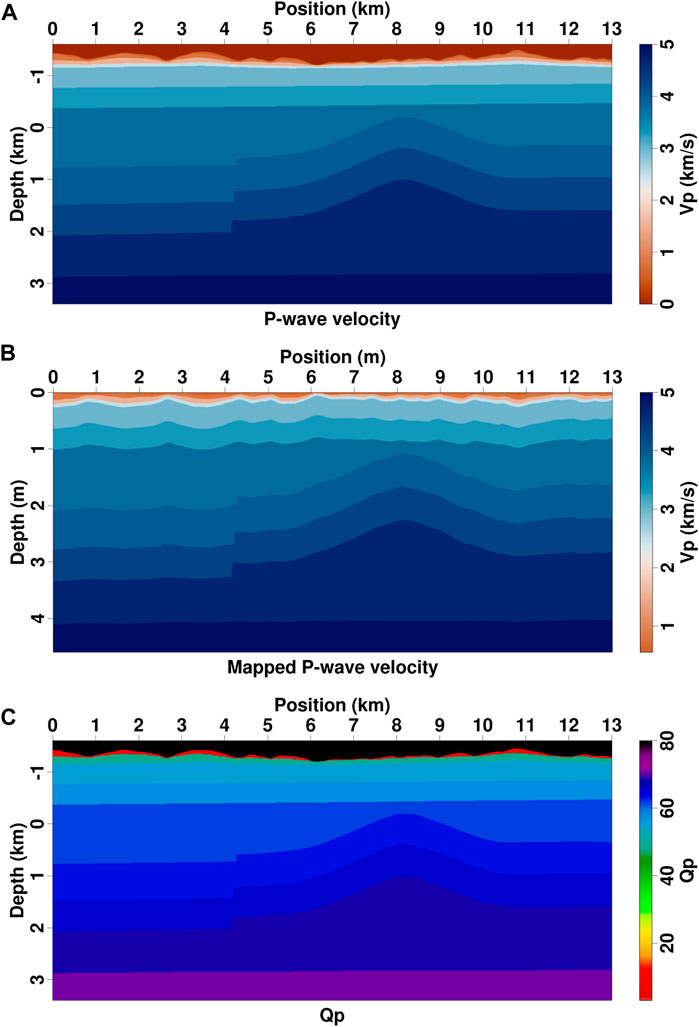
FIGURE 10. 2D Loess Plateau model. (A) P-wave velocity model, (B) mapped velocity model in the computational domain, and (C) quality factor Q model. The Q value above topography is 1,000 and is clipped to 80 for plotting.
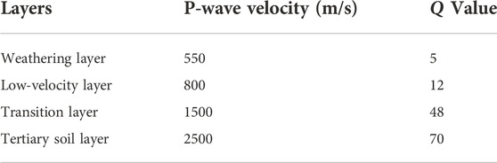
TABLE 2. P-wave velocity and Q values of loess layers.
The snapshots in the computational domain and physical space computed with and without the free surface are shown in Figures 11, 12. With a top absorption boundary condition, the reflected waves of subsurface interfaces can be clearly distinguished from direct waves (Figure 11). The wavefronts in the computational domain are slightly distorted and appear to be non-continuous because of irregular topography (left column in Figure 11). After mapping back to the physical domain, the wavefields, especially for reflections, have regular half-circle wavefronts (right column in Figure 11). By setting the topography as a free surface, seismic waves propagate back and forth between top surface and loess bottom vertically and between hill and ditch horizontally, resulting in strong multiple-like scatterings. These scatterings contaminate effective reflections generated from deep interfaces (Figure 12). Comparisons between acoustic and viscoacoustic modeling show a similar result as in the example of layer model (Figure 13). Their waveforms are similar when the propagation time is less than 0.5 s (Figure 13A). But as the time increases to 1 s, the difference of phases and amplitudes can be visually observed (Figure 13B). With a further longer duration, viscoacoustic wavefields have considerably weaker amplitudes than acoustic modeling results (Figures 13C,D).
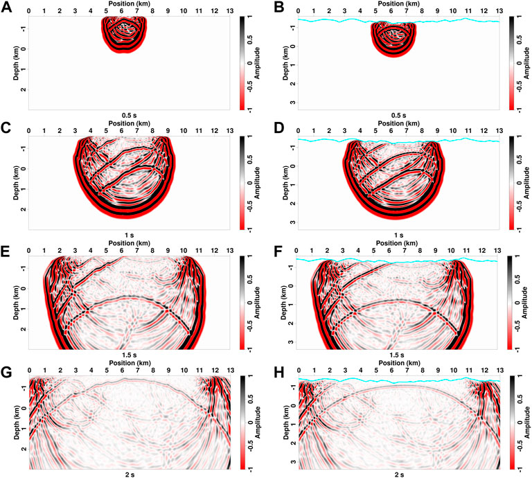
FIGURE 11. (A–H) Viscoacoustic wavefields of 2D Loess Plateau model at different propagation times simulated with a top absorption boundary in the computational domain (left column) and physical domain (right column). The cyan lines in panels (B,D,F, and H) denote the topography.
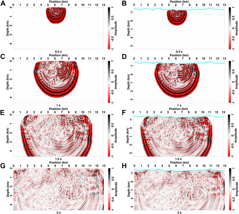
FIGURE 12. (A–H) Viscoacoustic wavefields of different propagation times for the 2D Loess Plateau model simulated with a top free-surface boundary in the computational domain (left column) and physical domain (right column). The cyan lines in panels (B,D,F, and H) denote the topography.
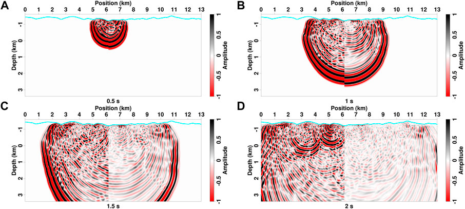
FIGURE 13. (A–D) Comparison of acoustic (left half panel) and viscoacoustic (right half panel) wavefields for the 2D Loess Plateau model at different propagation times. The cyan lines denote the topography.
The corresponding common-shot gathers are presented in Figure 14. Large velocity contrasts between loess layers and basement produce complicated refractions around the first break, and irregular topography results in distorted non-hyperbolic reflections (Figure 14A). Incorporating the free surface into viscoacoustic modeling produces strong scattering noises near the direct wave, and deep effective reflections are totally submerged in the noise (Figure 14B). For comparison, we also compute acoustic records using the same model and observation settings. Similar to the analysis for snapshots, the events at a short time have similar phases and amplitudes on acoustic and viscoacoustic records (Figures 14C,D). But considerable difference of deep reflections can be observed as the time increases due to attenuation-related phase dispersion and amplitude dissipation. In addition, large-offset refractions and scatterings near direct wave of viscoacoustic record are much weaker than those of acoustic modeling results. This is caused by strong attenuation in the low-Q loess layers.
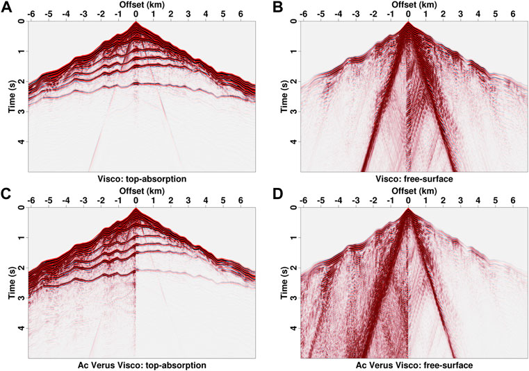
FIGURE 14. Common-shot gathers of 2D Loess Plateau model (A,B) Viscoacoustic modeling with top absorption and free surface boundaries, (C,D) comparison of acoustic (left half panel) and viscoacoustic (right half panel) records computed with top absorption and free surface boundaries.
3D Loess Plateau model
Because 2D modeling cannot accurately simulate the amplitudes of seismic waves, we apply the proposed viscoacoustic modeling method to a more realistic 3D model (Figure 15). Compared with 2D Loess Plateau model, geographic characteristics of loess distribution, including typical ditch, hill and valley, are more clearly visible in the 3D model. The setting for Q in shallow loess layers is the same to that in 2D model. For deep sandstone strata, the well-logging data and rock physics analysis show that P-wave velocity and Q models crudely satisfy an empirical relation as
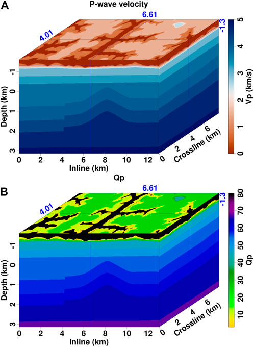
FIGURE 15. 3D Loess Plateau model. (A) P-wave velocity, and (B) Q model. The Q value above topography is 1,000 and is clipped to 80 for plotting.
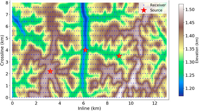
FIGURE 16. Source and receiver distributions of three observation systems for 3D wavefield models. Red stars denote the source locations of three experiments at the ditch (1), hill (2) and valley (3), and blue dots denote receivers.
The snapshots and common-shot gathers are presented in Figures 17, 18. Similar to 2D modeling, the interactions between topographic free-surface and loess bottom produces strong scatterings in near-surface region, which contaminate deep reflections (Figure 17). This leads to typical “black-triangle” noise below the source location in the records (Figure 18A). Without subsequent processing, it is difficult to visually find hyperbolic reflections. Because of the geometric spreading in a 3D volume, wavefield amplitude decays faster during propagation than in the 2D case. In addition, seismic attenuation introduces strong amplitude dissipation for viscoacoustic waves (right column in Figure 17). This results in rather weak amplitudes at large-offset traces and large observation time compared with acoustic recordings (Figures 18B,C).
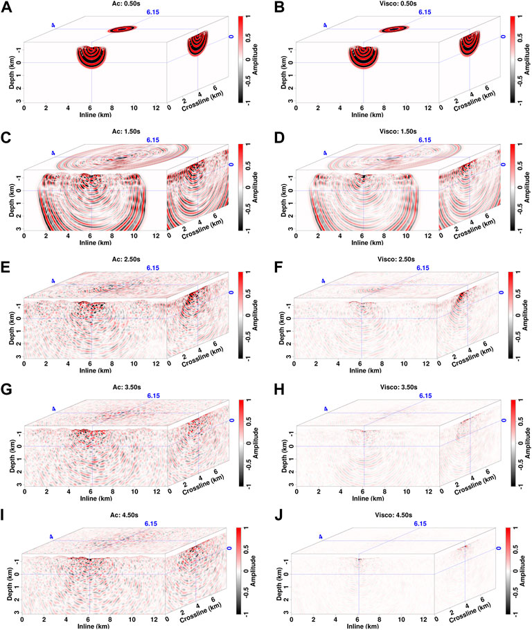
FIGURE 17. Comparison of acoustic (A,C,E,G,I) and viscoacoustic (B,D,F,H,J) wavefields with the source location at the ditch (No. 1 in Figure 16).
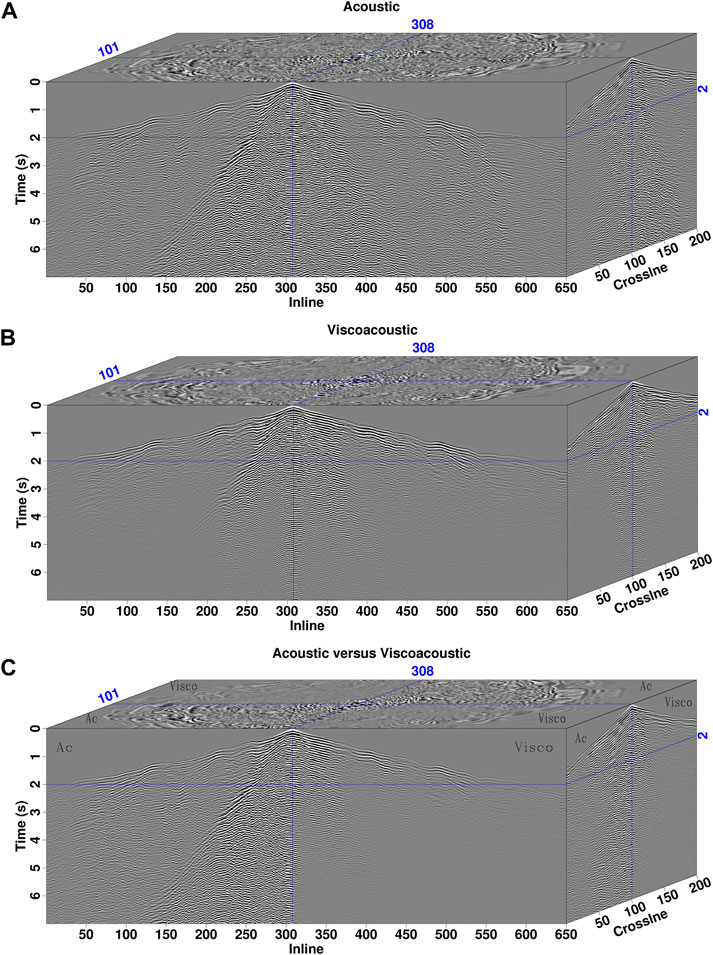
FIGURE 18. Common-shot gathers of 3D Loess Plateau model with the source location at the ditch. (A) Acoustic modeling result, (B) viscoacoustic modeling result, and (C) comparison of acoustic (Ac) versus viscoacoustic (Visco) modeling results.
The modeling results of the other two experiments are shown in Figures 19–21. Thicker loess sediments in the hill and valley produce stronger attenuation effect on seismic waves than that in the ditch, resulting in large amplitude and phase difference between acoustic and viscoacoustic snapshots (Figure 19). The phase dispersion and amplitude dissipation of viscoacoustic recordings become more pronounced. The waveforms with large offsets and times, including near-surface-related scatterings and deep reflections, are attenuated quickly (Figures 20, 21). In contrast to acoustic recordings, no events can be observed visually at the time greater than 5 s. The low SNR and weak amplitudes of recordings pose a great challenge for subsequent seismic data processing and imaging.
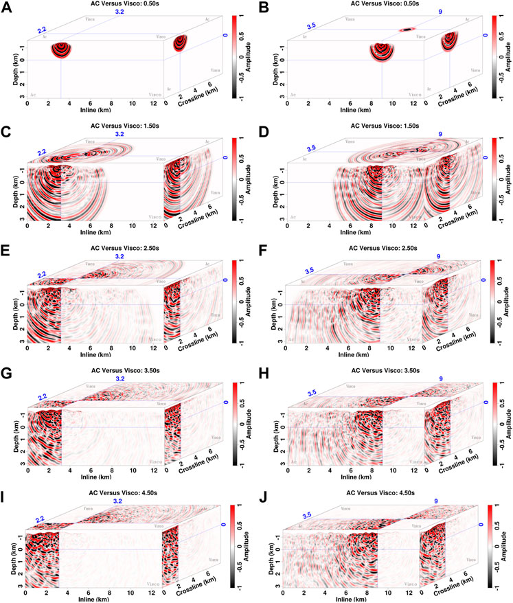
FIGURE 19. Comparison of acoustic and viscoacoustic wavefields with the source locations at the hill [(A,C,E,G,I), No. 2 in Figure 16] and valley [(B,D,F,H,J), No. 3 in Figure 16].
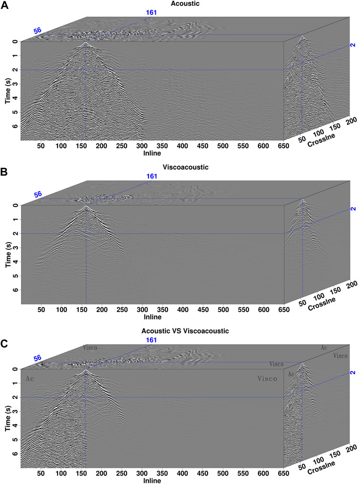
FIGURE 20. (A–C) Common-shot gathers of 3D Loess Plateau model with the source location at the hill. The panel notations are the same as those in Figure 18.
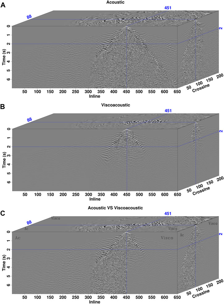
FIGURE 21. (A–C) Common-shot gathers of 3D Loess Plateau model with the source location at the valley. The panel notations are the same as those in Figure 18.
Figure 22 shows the snapshots of 1.5 s on the observation surface for three experiments. In the first experiment, strong scatterings are generated and propagate along the north-south ditch (Figures 22A,B). This is because the loess in the ditch was eroded, and the outcrop has a relative higher velocity than the loess. In contrast, the experiments excited on the hill and valley show an isotropic scattering pattern (Figures 22C–F). In addition, the wavefields excited by the source on the hill are affected by attenuation more largely than those excited in the ditch and valley (Figures 22D,F). Comparisons of acoustic modeling result, viscoacoustic modeling result and a common-shot gather acquired from Chinese Loess Plateau are presented in Figure 23. Note that both acoustic and viscoacoustic modeling can simulate strong black-triangle scattering noise below the direct waves, which has a consistent kinematic pattern with the field data. But acoustic records have relatively stronger amplitudes for the time greater than 3 s (Figure 23B). By incorporating seismic attenuation, viscoacoustic modeling produces weak amplitudes for large-duration and large-offset events, which have a good agreement with the amplitude characteristic of field data (Figure 23C).
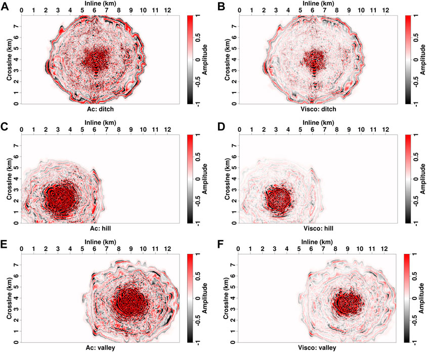
FIGURE 22. Acoustic (left column) and viscoacoustic (right column) wavefields on the topographic surface at 1.5 s. (A,B), (C,D), and (E,F) are the results excited by the source at three different locations, respectively.
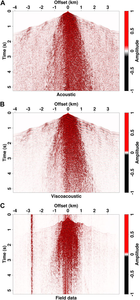
FIGURE 23. Comparison of synthetic common-shot gathers with field data acquired from Chinese Loess Plateau. (A) 3D acoustic modeling result, (B) 3D viscoacoustic modeling result, and (C) field data.
Discussion
To study wave propagations in the Loess Plateau, we propose a viscoacoustic modeling method based upon a wave equation with the explicitly expressed Q. It does not need to convert Q to strain and stress relaxation times as in the GSLS method. But compared with the fractional Laplacian complex-valued wave equations (Zhu and Harris, 2014; Yang and Zhu, 2018), the proposed equation does not separate the dispersion and dissipation terms. This makes it not as easy as Zhu and Harris (2014) and Yang and Zhu (2018)’s methods to directly compensate for Q effect in the reverse-time migration. An appropriate Q-compensation strategy will be investigated for seismic imaging in the future.
In this study, we do not incorporate the elasticity and anisotropy into wavefield modeling, and therefore cannot simulate S-wave propagation and P-S conversion. More accurate wavefield simulation should be extended to an anisotropic and anelastic medium, which can describe both P- and S-wave propagations in the Loess Plateau. But for elastic modeling, the S-wave velocity of loess layers can be as low as 200–300 m/s. This requires a very fine grid (
From 2D/3D modeling results for the Loess Plateau model, there is strong black-triangle scattering noise below the direct waves, which is consistent with the field observation. The generation mechanism of this type noise is similar to that of interval multiples, which results from the wave propagation back and forth between top free surface and loess bottom vertically and between hill and ditch horizontally. If incorporating elasticity in the modeling, surface waves will interact with the scatterings and produce more complicated noise. In subsequent processing, it is critical to remove the effect of strong black-triangle noise to produce a high-quality image, and therefore advanced signal processing techniques should be adopted to suppress loess-related noise.
Conclusion
We present a 2D/3D viscoacoustic modeling method in this work and apply it to simulate wave propagation in the Loess Plateau. A viscoacoustic wave equation with the explicitly expressed Q is first derived to describe the phase dispersion and amplitude dissipation. Then, a vertically deformed grid is used to conforms to the topographic surface, which build a mapping relation between physical space and computational domain. To accurately computed the spatial derivatives, a fully staggered-grid finite-difference scheme is utilized to solve the viscoacoustic wave equation in the deformed grid. Numerical experiments demonstrate that the proposed method can accurately simulate viscoacoustic wave propagation in the Loess Plateau models. The 3D modeling results show consistent kinematic and dynamic characteristics with the field data acquired from the Loess Plateau in China.
Data availability statement
The original contributions presented in the study are included in the article/supplementary material, further inquiries can be directed to the corresponding author.
Author contributions
ZH presented the idea, JY, LH, JH, and SQ developed the code, did the tests and wrote the manuscript. JS and YY revised the manuscript.
Funding
This study is funded by the CNPC project of viscoacoustic wave equation modeling and reverse-time migration (no. HX20220326), and the startup funding (no. 20CX06069A) of Guanghua Scholar at China University of Petroleum (East China). The work was carried out at National Supercomputer Center in Tianjin, and this research was supported by Tianhe Qingsuo Project-special fund project in the field of geoscience.
Acknowledgments
We are thankful for the support from the Funds of the National Key R&D Program of China (no. 2019YFC0605503), the Major Scientific and Technological Projects of CNPC (no. ZD 2019-183-003), the Major projects during the 14th Five-year Plan period (no. 2021QNLM020001), the National Outstanding Youth Science Foundation (no. 41922028), and Creative Research Groups of China (no. 41821002).
Conflict of interest
The authors ZH and LH were employed by Research Institute of Petroleum Exploration and Development-Northwest PetroChina.
The remaining authors declare that the research was conducted in the absence of any commercial or financial relationships that could be construed as a potential conflict of interest.
Publisher’s note
All claims expressed in this article are solely those of the authors and do not necessarily represent those of their affiliated organizations, or those of the publisher, the editors and the reviewers. Any product that may be evaluated in this article, or claim that may be made by its manufacturer, is not guaranteed or endorsed by the publisher.
References
Aki, K., and Richards, P. G. (2002). Quantitative seismology. United States: University Science Books.
Beydoun, W. B., and Keho, T. H. (1987). The paraxial ray method. Geophysics 52, 1639–1653. doi:10.1190/1.1442281
Bording, R. P., and Lines, L. R. (1997). Seismic modeling and imaging with the complete wave equation. Houston, Texas, United States: Society of Exploration Geophysicists.
Carcione, J. M., Herman, G. C., and ten Kroode, A. P. E. (2002). Seismic modeling. Geophysics 67, 1304–1325. doi:10.1190/1.1500393
Carcione, J. M., Poletto, F., and Gei, D. (2004). 3-D wave simulation in anelastic media using the Kelvin–Voigt constitutive equation. J. Comput. Phys. 196, 282–297. doi:10.1016/j.jcp.2003.10.024
Carcione, J. M. (1993). Seismic modeling in viscoelastic media. Geophysics 58, 110–120. doi:10.1190/1.1443340
Carcione, J. M. (2007). Wave fields in real media: Wave propagation in anisotropic, anelastic, porous and electromagnetic media. Amsterdam, Netherlands: Elsevier.
Carcione, J. M. (1990). Wave propagation in anisotropic linear viscoelastic media: Theory and simulated wavefields. Geophys. J. Int. 101, 739–750. doi:10.1111/j.1365-246X.1990.tb05580.x
Červený, V., Klimeš, L., and Pšenčík, I. (2007). “Seismic ray method: Recent developments,” in Advances in wave propagation in heterogenous Earth. Editors R.-S. Wu, V. Maupin, and R. Dmowska (Amsterdam, Netherlands: Elsevier), 1–126. doi:10.1016/S0065-2687(06)48001-8
Červený, V., Popov, M. M., and Pšenčík, I. (1982). Computation of wave fields in inhomogeneous media-Gaussian beam approach. Geophys. J. Int. 70, 109–128. doi:10.1111/j.1365-246x.1982.tb06394.x
Chapman, H., and Drummond, R. (1982). Body-wave seismograms in inhomogeneous media using Maslov asymptotic theory. Bull. Seismol. Soc. Am. 72, S277–S317. doi:10.1785/BSSA07206B0277
Chen, H., Zhou, H., Li, Q., and Wang, Y. (2016). Two efficient modeling schemes for fractional Laplacian viscoacoustic wave equation. GEOPHYSICS 81, T233–T249. doi:10.1190/geo2015-0660.1
De Basabe, J. D., and Sen, M. K. (2009). New developments in the finite-element method for seismic modeling. Lead. Edge 28, 562–567. doi:10.1190/1.3124931
de la Puente, J., Ferrer, M., Hanzich, M., Castillo, J. E., and Cela, J. M. (2014). Mimetic seismic wave modeling including topography on deformed staggered grids. Geophysics 79, T125–T141. doi:10.1190/geo2013-0371.1
Emmerich, H., and Korn, M. (1987). Incorporation of attenuation into time-domain computations of seismic wave fields. GEOPHYSICS 52, 1252–1264. doi:10.1190/1.1442386
Etgen, J. T., and O’Brien, M. J. (2007). Computational methods for large-scale 3D acoustic finite-difference modeling: A tutorial. Geophysics 72, SM223–SM230. doi:10.1190/1.2753753
Fichtner, A., and van Driel, M. (2014). Models and fréchet kernels for frequency-(in)dependent q. Geophys. J. Int. 198, 1878–1889. doi:10.1093/gji/ggu228
Gray, S. H., and May, W. P. (1994). Kirchhoff migration using eikonal equation traveltimes. Geophysics 59, 810–817. doi:10.1190/1.1443639
Guo, P., and Mcmechan, G. A. (2017). Evaluation of three first-order isotropic viscoelastic formulations based on the generalized standard linear solid. J. Seismic Explor. 26, 199–226.
Guo, P., McMechan, G. A., and Ren, L. (2019). Modeling the viscoelastic effects in p-waves with modified viscoacoustic wave propagation. Geophysics 84, T381–T394. doi:10.1190/geo2018-0747.1
Hestholm, S., and Ruud, B. (1994). 2D finite-difference elastic wave modelling including surface topography1. Geophys. Prospect. 42, 371–390. doi:10.1111/j.1365-2478.1994.tb00216.x
Hestholm, S., and Ruud, B. (1998). 3-D finite-difference elastic wave modeling including surface topography. Geophysics 63, 613–622. doi:10.1190/1.1444360
Hestholm, S., and Ruud, B. (2002). 3d free-boundary conditions for coordinate-transform finite-difference seismic modelling. Geophys. Prospect. 50, 463–474. doi:10.1046/j.1365-2478.2002.00327.x
Hestholm, S. (1999). Three-dimensional finite difference viscoelastic wave modelling including surface topography. Geophys. J. Int. 139, 852–878. doi:10.1046/j.1365-246x.1999.00994.x
Hill, R. (2001). Prestack Gaussian-beam depth migration. Geophysics 66, 1240–1250. doi:10.1190/1.1487071
Jastram, C., and Tessmer, E. (1994). Elastic modelling on a grid with vertically varying spacing1. Geophys. Prospect. 42, 357–370. doi:10.1111/j.1365-2478.1994.tb00215.x
Kendall, J., and Thomson, C. (1993). Maslov ray summation, pseudo-caustics, Lagrangian equivalence and transient seismic waveforms. Geophys. J. Int. 113, 186–214. doi:10.1111/j.1365-246x.1993.tb02539.x
Kjartansson, E. (1979). Constant Q-wave propagation and attenuation. J. Geophys. Res. 84, 4737–4748. doi:10.1029/JB084iB09p04737
Koene, E. F. M., Robertsson, J. O. A., and Andersson, F. (2021). Anisotropic elastic finite-difference modeling of sources and receivers on Lebedev grids. Geophysics 86, A21–A25. doi:10.1190/geo2020-0522.1
Komatitsch, D., Barnes, C., and Tromp, J. (2000). Simulation of anisotropic wave propagation based upon a spectral element method. Geophysics 65, 1251–1260. doi:10.1190/1.1444816
Komatitsch, D., Erlebacher, G., Göddeke, D., and Michéa, D. (2010). High-order finite-element seismic wave propagation modeling with mpi on a large gpu cluster. J. Comput. Phys. 229, 7692–7714. doi:10.1016/j.jcp.2010.06.024
Komatitsch, D., Ritsema, J., and Tromp, J. (2002). The spectral-element method, beowulf computing, and global seismology. Science 298, 1737–1742. doi:10.1126/science.1076024
Komatitsch, D., and Tromp, J. (1999). Introduction to the spectral element method for three-dimensional seismic wave propagation. Geophys. J. Int. 139, 806–822. doi:10.1046/j.1365-246x.1999.00967.x
Komatitsch, D., and Tromp, J. (2002). Spectral-element simulations of global seismic wave propagation—I. Validation. Geophys. J. Int. 149, 390–412. doi:10.1046/j.1365-246X.2002.01653.x
Konuk, T., and Shragge, J. (2020). Modeling full-wavefield time-varying sea-surface effects on seismic data: A mimetic finite-difference approach. Geophysics 85, T45–T55. doi:10.1190/geo2019-0181.1
Kristek, J., and Moczo, P. (2003). Seismic-wave propagation in viscoelastic media with material discontinuities: A 3D fourth-order staggered-grid finite-difference modeling. Bull. Seismol. Soc. Am. 93, 2273–2280. doi:10.1785/0120030023
Lebedev, V. (1964). Difference analogues of orthogonal decompositions, basic differential operators and some boundary problems of mathematical physics. i. USSR Comput. Math. Math. Phys. 4, 69–92. doi:10.1016/0041-5553(64)90240-X
Lei, W., Ruan, Y., Bozda, E., Peter, D., Lefebvre, M., Komatitsch, D., et al. (2020). Global adjoint tomography—Model GLAD-M25. Geophys. J. Int. 223, 1–21. doi:10.1093/gji/ggaa253
Levander, A. R. (1988). Fourth-order finite-difference p-sv seismograms. Geophysics 53, 1425–1436. doi:10.1190/1.1442422
Liao, Q., and McMechan, G. A. (1996). Multifrequency viscoacoustic modeling and inversion. Geophysics 61, 1371–1378. doi:10.1190/1.1444060
Lisitsa, V., and Vishnevskiy, D. (2010). Lebedev scheme for the numerical simulation of wave propagation in 3d anisotropic elasticity. Geophys. Prospect. 58, 619–635. doi:10.1111/j.1365-2478.2009.00862.x
Liu, H.-P., Anderson, D. L., and Kanamori, H. (1976). Velocity dispersion due to anelasticity: Implications for seismology and mantle composition. Geophys. J. Int. 47, 41–58. doi:10.1111/j.1365-246X.1976.tb01261.x
Marfurt, K. J. (1984). Accuracy of finite-difference and finite-element modeling of the scalar and elastic wave equations. Geophysics 49, 533–549. doi:10.1190/1.1441689
Maslov, V., Arnold, V., and Buslaev, V. S. (1972). Theory of perturbations and asymptotic methods. Russia: Moscow University Press.
McMechan, G. A. (1989). A review of seismic acoustic imaging by reverse-time migration. Int. J. Imaging Syst. Technol. 1, 18–21. doi:10.1002/ima.1850010104
Mittet, R. (2002). Free-surface boundary conditions for elastic staggered-grid modeling schemes. Geophysics 67, 1616–1623. doi:10.1190/1.1512752
Mulder, W., and Plessix, R. (2008). Exploring some issues in acoustic full waveform inversion. Geophys. Prospect. 56, 827–841. doi:10.1111/j.1365-2478.2008.00708.x
Müller, G. (1984). Efficient calculation of Gaussian-beam seismograms for two-dimensional inhomogeneous media. Geophys. J. Int. 79, 153–166. doi:10.1111/j.1365-246x.1984.tb02847.x
Nakamura, T., Takenaka, H., Okamoto, T., and Kaneda, Y. (2012). Fdm simulation of seismic-wave propagation for an aftershock of the 2009 suruga bay earthquake: Effects of ocean-bottom topography and seawater layer. Bull. Seismol. Soc. Am. 102, 2420–2435. doi:10.1785/0120110356
Nowack, R., and Aki, K. (1984). The two-dimensional Gaussian beam synthetic method: Testing and application. J. Geophys. Res. 89, 7797–7819. doi:10.1029/jb089ib09p07797
Robertsson, J. O. (1996). A numerical free-surface condition for elastic/viscoelastic finite-difference modeling in the presence of topography. Geophysics 61, 1921–1934. doi:10.1190/1.1444107
Shragge, J., and Tapley, B. (2017). Solving the tensorial 3d acoustic wave equation: A mimetic finite-difference time-domain approach. Geophysics 82, T183–T196. doi:10.1190/geo2016-0691.1
Sjögreen, B., and Petersson, N. A. (2012). A fourth order accurate finite difference scheme for the elastic wave equation in second order formulation. J. Sci. Comput. 52, 17–48. doi:10.1007/s10915-011-9531-1
Stekl, I., and Pratt, R. G. (1998). Accurate viscoelastic modeling by frequency-domain finite differences using rotated operators. Geophysics 63, 1779–1794. doi:10.1190/1.1444472
Sun, J. (2002). Provenance of loess material and formation of loess deposits on the Chinese loess plateau. Earth Planet. Sci. Lett. 203, 845–859. doi:10.1016/S0012-821X(02)00921-4
Sun, J., Zhu, T., and Fomel, S. (2015). Viscoacoustic modeling and imaging using low-rank approximation. Geophysics 80, A103–A108. doi:10.1190/geo2015-0083.1
Sun, Y., Zhang, W., and Chen, X. (2016). Seismic-wave modeling in the presence of surface topography in 2D general anisotropic media by a curvilinear grid finite-difference method. Bull. Seismol. Soc. Am. 106, 1036–1054. doi:10.1785/0120150285
Sun, Y., Zhang, W., Ren, H., Bao, X., Xu, J., Sun, N., et al. (2021). 3D seismic-wave modeling with a topographic fluid–solid interface at the sea bottom by the curvilinear-grid finite-difference method. Bull. Seismol. Soc. Am. 111, 2753–2779. doi:10.1785/0120200363
Tape, C., Liu, Q., Maggi, A., and Tromp, J. (2009). Adjoint tomography of the southern California crust. Science 325, 988–992. doi:10.1126/science.1175298
Um, J., and Thurber, C. (1987). A fast algorithm for two-point seismic ray tracing. Bull. Seismol. Soc. Am. 77, 972–986. doi:10.1785/BSSA0770030972
Vigh, D., Starr, E. W., and Kapoor, J. (2009). Developing Earth models with full waveform inversion. Lead. Edge 28, 432–435. doi:10.1190/1.3112760
Virieux, J., and Operto, S. (2009). An overview of full-waveform inversion in exploration geophysics. Geophysics 74, WCC1–WCC26. doi:10.1190/1.3238367
Virieux, J., Operto, S., Ben-Hadj-Ali, H., Brossier, R., Etienne, V., Sourbier, F., et al. (2009). Seismic wave modeling for seismic imaging. Lead. Edge 28, 538–544. doi:10.1190/1.3124928
Virieux, J. (1986). P-SV wave propagation in heterogeneous media: Velocity-stress finite-difference method. Geophysics 51, 889–901. doi:10.1190/1.1442147
Wang, D., Gao, J., Li, Y., Xia, Z., and Wang, B. (2004). Mesozoic reservoir prediction in the longdong loess plateau. Appl. Geophys. 1, 20–25. doi:10.1007/s11770-004-0023-z
Wang, N., Xing, G., Zhu, T., Zhou, H., and Shi, Y. (2022). Propagating seismic waves in vti attenuating media using fractional viscoelastic wave equation. JGR. Solid Earth 127, e2021JB023280. doi:10.1029/2021jb023280
Wang, X., Zhang, L., Liang, Q., Jiang, C., Wang, W., Xiaolong, Y., et al. (2014). Full-azimuth, high-density, 3d point-source/point-receiver seismic survey for shale gas exploration in a Loess Plateau: A case study from the ordos basin, China. United States: First Break, 32.
Wang, Z., Li, J., Wang, B., Xu, Y., and Chen, X. (2017). Time-domain explicit finite-difference method based on the mixed-domain function approximation for acoustic wave equation. Geophysics 82, T237–T248. doi:10.1190/geo2017–0012.1
Wu, W., Lines, L. R., and Lu, H. (1996). Analysis of higher-order, finite-difference schemes in 3-D reverse-time migration. Geophysics 61, 845–856. doi:10.1190/1.1444009
Xing, G., and Zhu, T. (2019). Modeling frequency-independent q viscoacoustic wave propagation in heterogeneous media. J. Geophys. Res. Solid Earth 124, 11568–11584. doi:10.1029/2019jb017985
Yang, D., Liu, E., Zhang, Z., and Teng, J. (2002). Finite-difference modelling in two-dimensional anisotropic media using a flux-corrected transport technique. Geophys. J. Int. 148, 320–328. doi:10.1046/j.1365-246x.2002.01012.x
Yang, J., Huang, J., Zhu, H., McMechan, G., and Li, Z. (2022). Introduction to a two-way beam wave method and its applications in seismic imaging. JGR. Solid Earth 127, e2021JB023357. doi:10.1029/2021jb023357
Yang, J., and Zhu, H. (2018). A time-domain complex-valued wave equation for modelling visco-acoustic wave propagation. Geophys. J. Int. 215, 1064–1079. doi:10.1093/gji/ggy323
Yang, J., Zhu, H., Li, X., Ren, L., and Zhang, S. (2020). Estimating p wave velocity and attenuation structures using full waveform inversion based on a time domain complex-valued viscoacoustic wave equation: The method. J. Geophys. Res. Solid Earth 125, e2019JB019129. doi:10.1029/2019jb019129
Yang, J., Zhu, H., McMechan, G., and Yue, Y. (2018). Time-domain least-squares migration using the Gaussian beam summation method. Geophys. J. Int. 214, 548–572. doi:10.1093/gji/ggy142
Yao, J., Zhu, T., Hussain, F., and Kouri, D. J. (2017). Locally solving fractional laplacian viscoacoustic wave equation using hermite distributed approximating functional method. Geophysics 82, T59–T67. doi:10.1190/geo2016–0269.1
Zhang, W., Zhang, Z., and Chen, X. (2012). Three-dimensional elastic wave numerical modelling in the presence of surface topography by a collocated-grid finite-difference method on curvilinear grids. Geophys. J. Int. 190, 358–378. doi:10.1111/j.1365-246X.2012.05472.x
Appendix A: Stability condition for the finite-difference onto a vertical stretched grid
According the energy analysis method (Yang et al., 2002), the stability of the finite-difference solver for Eq. 13 requires the time and space increments satisfying
If the spatial increments are the same, i.e., Δh = Δα = Δβ = Δγ, we have
Incorporating the finite-difference coefficients, the time interval has to satisfy
where c is the summation of finite-difference coefficients. Considering the varying velocity, Q and topography slope, Eq. A3 reduces to Eq. 14.
Keywords: viscoacoustic modeling, seismic wave attenuation, Loess Plateau, topographic surface, computational seismology
Citation: Hu Z, Yang J, Han L, Huang J, Qin S, Sun J and Yu Y (2023) Modeling seismic wave propagation in the Loess Plateau using a viscoacoustic wave equation with explicitly expressed quality factor. Front. Earth Sci. 10:1069166. doi: 10.3389/feart.2022.1069166
Received: 13 October 2022; Accepted: 15 November 2022;
Published: 27 January 2023.
Edited by:
Mourad Bezzeghoud, Universidade de Évora, PortugalReviewed by:
Lin Zhang, Hohai University, ChinaJiajia Zhangjia, China University of Petroleum, China
Copyright © 2023 Hu, Yang, Han, Huang, Qin, Sun and Yu. This is an open-access article distributed under the terms of the Creative Commons Attribution License (CC BY). The use, distribution or reproduction in other forums is permitted, provided the original author(s) and the copyright owner(s) are credited and that the original publication in this journal is cited, in accordance with accepted academic practice. No use, distribution or reproduction is permitted which does not comply with these terms.
*Correspondence: Jidong Yang, amlkb25nLnlhbmdAdXBjLmVkdS5jbg==