 Honglei Li
 Shi Chen
 Yongbo Li
 Bei Zhang1,2
 Ming Zhao
- 1Institute of Geophysics, China Earthquake Administration, Beijing, China
- 2Beijing Baijiatuan Earth Science National Observation and Research Station, Beijing, China
Downward continuation (DC) of the gravity potential field is an important approach used to understand and interpret the density structure and boundary of anomalous bodies. It is widely used to delineate and highlight local and shallow anomalous sources. However, it is well known that direct DC transformation in the frequency domain is unstable and easily affected by high-frequency noise. Recent deep learning applications have led to the development of image recognition and resolution enhancement using the convolutional neural network technique. A similar deep learning architecture is also suitable for training a model for the DC problem. In this study, to solve the problems in existing DC methods, we constructed a dedicated model called DC-Net for the DC problem. We fully trained the DC-Net model on 38,400 pairs of gravity anomaly data at different altitudes using a convolutional neural network. We conducted several experiments and implemented a real-world example. The results demonstrate the following. First, several validation data subset and test data prediction results indicate that the DC-Net model was sufficiently trained. Moreover, it performed better than the traditional strategy in refining the upscaling of low-resolution images. Second, we performed tests on test datasets with changing levels of noise and demonstrated that the DC-Net model is noise-resistant and robust. Finally, we used the proposed model in a real-world example, which demonstrates that the DC-Net model is suitable for solving the DC problem and delineating the detailed gravity anomaly feature near the field source. For real data processing, noise in the gravity anomaly should be reduced in advance. Additionally, we recommend noise quantification of the gravity anomaly before network training.
1 Introduction
Downward continuation (DC) of the gravity potential field is an important processing and interpretation approach used to enhance the local and shallow signal of a deep field source. It is widely used in, for example, the exploration of minerals, oil and gas basin analysis, and assisted navigation (Cordell and Grauch, 1985; Blakely, 1996; Adewumi and Salako, 2018). At present, many algorithms exist for the DC problem, which can be roughly divided into three categories: the spatial domain interpolation method (e.g., Cooper, 2004; Luo and Wu, 2016), the wavenumber domain method (e.g., Liu et al., 2009; Zhou et al., 2022), and the integral iterative method (e.g., Ma et al., 2013; Tai et al., 2016; Chen and Yang, 2022). Although many existing methods have achieved certain effects in some geophysical interpretations, two unsolved problems remain in existing methods. One problem is inevitable boundary errors. Because of the limitations of geophysical observations, regardless of whether the DC operator is solved in the space domain or wavenumber domain, the calculated plane cannot be infinite, and the calculation of the Gibbs effect is unavoidable, which results in boundary position errors (Pašteka et al., 2012). The other unsolved problem is unstable calculation. The results derived by the DC operator include more high-frequency characteristics and short wavelength anomaly components than the untransformed data because the result derived by the DC operator is closer to the anomalous sources than the untransformed data. However, the DC operator also significantly increases noise and results in an unstable continuation computation (Zhang et al., 2009; Zeng et al., 2011). Both problems can be attributed to the incorrect solution of the DC operator.
Recent advancements in the development of deep learning (DL) provide a good method for solving the aforementioned problems. The DC operator can be regarded as the mapping relationship between two gravity anomalies. DL can obtain the mapping relationship though a massive data-driven approach, which provides the DL method with the potential to achieve a more accurate predictive effect than conventional approaches (Goodfellow et al., 2016). The convolutional neural network (CNN) is gradually becoming the most widely used computational approach in the DL field (Alzubaidi et al., 2021). In the last few years, the CNN method has been widely adopted in various geophysical scenarios (Bergen et al., 2019), such as exploration geophysics (e.g., Yang and Ma, 2019; Yu et al., 2019; Zhang et al., 2021; Wang et al., 2021), waveform classification and seismic recognition (e.g., Zhao et al., 2019; Zhu et al., 2019), and seismic image enhancement (Halpert, 2018; Wang and Nealon, 2019).
Therefore, in this study, we introduce a dedicated model called DC-Net that uses the U-net network (Ronneberger et al., 2015) for the DC of the gravity anomaly to solve the problems in existing DC methods. We trained the DC-Net model using many high-resolution gravity anomaly maps located at a low altitude, with their low-resolution counterparts at a high altitude. We then conducted extensive experiments on validation datasets and test datasets to illustrate the validity of the DC-Net model. We also used several test datasets with changing levels of noise to test the noise resistance of the model. Finally, we evaluated the method by applying it to a real airborne gravity (AG) anomaly and compared two continuations predicted by different trained models.
2 Methods
We divide the description of the methodology into two parts: DC theory and the critical components of the DC network (DC-Net).
2.1 DC problem for gravity
The DC of the potential field is used to obtain the potential field
As shown in Figure 1,
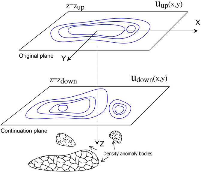
FIGURE 1. Schematic diagram of the DC problem.
Generally, the DC problem refers to the solution of the following boundary value problem (Blakely, 1996):
where h is the given continuation height, h =
where
Recent advancements in the development of machine learning (ML) provide a good approach for solving this problem. Different from traditional methods, ML is a type of data-driven approach that trains a regression model through complex nonlinear mapping with adjustable parameters using a training dataset (Goodfellow et al., 2016; Yu et al., 2019). In ML, the aforementioned DC problem can be described as
where
where
2.2 DC-Net
2.2.1 Structure of DC-Net
As shown in Figure 2, our DC-Net is primarily composed of four components: pre-processing, encoder, decoder, and post-processing. Pre-processing comprises two identical modules, each of which consists of two convolutional layers and two normalization-activation layers. We use this part to extract and activate the coarse pattern feature from the low-resolution input. The encoder and decoder have three identical modules. Each encoder module is composed of one convolutional layer, followed by one normalization-activation layer and one pooling layer. The role of the encoder is to prevent overfitting while maintaining high sampling rates. Each decoder module is sequentially composed of one deconvolution layer and one convolution layer, each of which is followed by one normalization-activation layer. The function of the decoder is to upsample the feature map size. However, post-processing has two different modules. The first is composed of two convolutional layers, followed by two normalization-activation layers, whereas the second only has a single convolutional layer. This part is used to output the result.
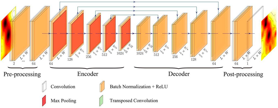
FIGURE 2. Structure of DC-Net.
The success of DC-Net is attributed to some practical “tricks.” First, rectified linear units (ReLUs) are used as the activation functions, which simply involves the half-wave rectifier function f(x) = max (x, 0), and can significantly accelerate the training phase. Second, the pooling method is maximum pooling, which is an effective approach for reducing overfitting when training a large CNN. Third, we construct several normalization-activation layers, followed by convolution and transposed convolution layers, which could mitigate numerical instability successfully.
The detailed procedure of the DC-Net model is illustrated in Table 1. We further use the PyTorch framework to complement the aforementioned operations and finally achieve the CNN-trained DC-Net model.
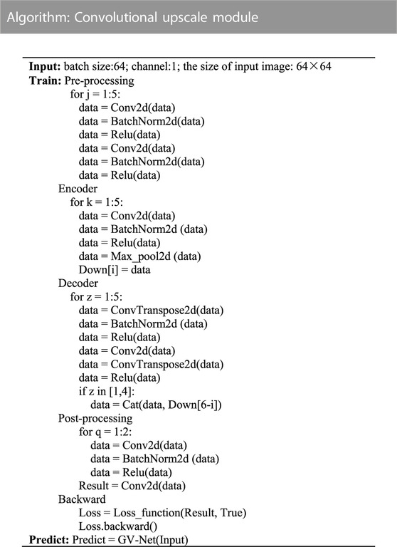
TABLE 1. DC-Net algorithm.
2.2.2 Loss function
During CNN training, we update the model parameters according to the definition of the loss function. Therefore, selecting a suitable loss function is critical for optimizing the updating of the model. There are traditional loss functions, such as L1, L2, and perceptual losses. The mean squared error (MSE) is one of the most common L2 loss functions, and it has been widely used in ML (Mao et al., 2017; Ghodrati et al., 2019; Zhang et al., 2020). We use the MSE loss function to express the deviation between the predicted DC gravity anomaly and the true value. Suppose there are
The aim of DC-Net is to minimize the loss function.
2.2.3 Metrics function
In addition to the loss function, there is another important function: the metrics function. The metrics function is similar to the loss function; both of them can be used to judge the performance of the training model. The only difference between the metrics function and the loss function is that metrics function is not used when training the model. Note that any loss function can be used as a metrics function. Including several kinds of loss functions mentioned before, metrics functions can be divided into several types, for instance, accuracy metrics (Han et al., 2022), probabilistic metrics (Branchaud-Charron et al., 2019), regression metrics (Geng et al., 2020), and so on. Compared to other metrics functions, the relative accurate function has a more intuitive expression and is more sensitive to changes in the accuracy of the predicted results. Therefore, in our DC-Net, we choose to use the relative accurate function to assess model accuracy:
The range of this metrics function is from 0 to 1; the more accurate the model prediction, the larger the value of ε.
3 Model training
3.1 Data generation
To train the DC-Net model, abundant training data need to be used to build the mapping relationship between the input and output. The quality of the training dataset directly determines the DC results of the model. In our DC-Net, we require two subsets of gravity data: one is the high-resolution gravity anomaly
In this study, we use a rectangular prism as the anomalous density source and present the theoretical gravity anomaly using that density model. The prism is bounded by planes parallel to the coordinate planes and defined by the coordinates
where
The size of each rectangular prism is 50 m × 100 m × 100 m. If the given rectangular prism has unit density, Green’s function matrix can be generated to map the discretized density bodies and gravity anomaly at the observation level. To simplify the training process of DC-Net, in our training model, we set
During DC-Net training, to ensure the diversity of gravity data samples, we consider the numbers of distinctive dataset distributions. First, the density models are composed of rectangular prisms of different scales and arrangements, with the density contrast varying randomly from 0.1 to 0.5 g/cm3. Second, we also include gravity datasets with boundary features in the training data to improve the prediction accuracy of boundary anomalies. Third, as the high-pass filtering property of the DC operator, we also add changing levels of Gaussian noise to the training dataset.
3.2 Training
For model training, we repeated the aforementioned data generation 76,800 times and finally used a total of 38,400 pairs of gravity anomaly datasets to feed our model. We divided these samples into three datasets: training dataset, validation dataset, and test dataset. The training dataset was composed of 90% of the entire dataset and the validation dataset was composed of a random selection of 10% of the training dataset.
We used the designed CNN as introduced in Section 2.2 to improve the generalization of our model. We set the maximum batch number to 128 for the global enhanced upscaled module. We used a low-resolution gravity image with 64 × 64 patches as single-channel input in each mini batch. Then, we gradually increased the number of channels to 64 during pre-processing and increased it to 1,204 in the encoder using three pooling processes while decreasing the patch number of each image from 64 × 64 to 4 × 4. In the decoder, we reduced the number of channels to 64 again and increased the patch number of each image to 64 × 64 again using three transposed convolution operations. Finally, in the output part, we set one gravity data channel with 64 × 64 patches as the output after two convolution operations.
For our training phase, we set the cutoff condition as the loss function less than 10–4 or the maximum epoch number less than 1,000. Moreover, we used the maximum pooling method in the backpropagation process to verify that the trained model was not overfitted. Our training ended after 600 epochs. The loss function curve and relative accuracy curve for the training dataset and validation dataset are shown in Figures 3A, B, respectively.
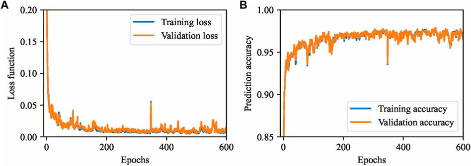
FIGURE 3. (A) Loss curve and (B) accuracy metric curves.
The loss function curves in Figure 3A show that both the training loss curve and validation loss curve decreased smoothly to a steady state as the training epochs increased. They gradually reduced to a small value of approximately 10–4 after 600 epochs, which indicates the successful convergence of our model. Furthermore, the training loss curve (orange curve) shows a slightly higher convergence value than the validation loss curve (blue curve), which means that the prediction fitting precision was affected by the fitting precision of the trained model and limited to a certain value.
The relative accuracy curves in Figure 3B show that the final DC prediction results had an accuracy value of over 0.95. The relative accuracy curve (orange curve) of the validation set shows almost the same accuracy as that of the training dataset (blue curve), which means that our DC-Net model achieved sufficiently accurate predictions, even for input that was not in the training set.
3.2.1 Synthetic test
We conducted several experiments to assess the effectiveness, noise immunity, and usability of our DC-Net model. The experiments and corresponding results are described as follows.
3.3 Validation datasets
We randomly selected a subset of the validation set to determine whether the validation set could be accurately predicted by our DC-Net model. The results are shown in Figure 4. As mentioned in Section 3.1, we set the two observation heights for all the training data to fixed height values of 500 m and 0 m. The same setting is also used in the validation data. Figure 4A is the map of the validation subset composed of several low-resolution gravity anomalies at 500 m, while Figure 4B is the map of the validation subset composed of the corresponding high-resolution gravity anomalies at 0 m, and Figure 4C shows the true value of gravity anomalies at 0 m. The continuation distance between them is a fixed value of 500 m. By comparing of the subset of validation data (Figure 4A), the prediction results of the subset (Figure 4B), and the true value of the prediction results (Figure 4C), we observed that our DC-Net has the ability to recover the shape of all the high-frequency signatures of the gravity anomalies. The predicted results (Figure 4B) are in good agreement with their true values (Figure 4C). Furthermore, complex boundary anomalies and gravity anomalies with significant noise pollution were also well recovered. This fully confirms that our trained DC-Net model has a good ability to avoid the phenomenon of the Gibbs effect and noise contamination.
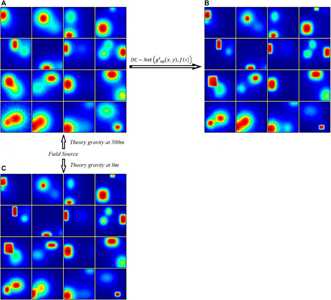
FIGURE 4. Validation dataset prediction effect display: (A) subset of the validation data composed of gravity anomalies at 500 m; (B) subset of the prediction results composed of gravity anomalies at 0 m; (C) true value of gravity anomalies at 0 m.
3.4 Test datasets
Subsequently, we conducted a test on a typical gravity dataset to verify the effect of different DC methods: the damped frequency DC (DFDC) method (Blakely, 1996), the Taylor series expansion DC (TEDC) method (Tran and Nguyen, 2020), and our DC-Net model.
The fundamental principles of the DFDC method are follows: for the continuation problem in Eq. 2, we assume that
which can be expressed in the form of
where
where
Then, we can obtain the solution of the DC problem as
However, the DC problem is an ill-posed problem, and the solution is usually unstable. To ensure the stability of the DC calculation, the trade-off parameter
The TEDC method is a newly published DC method for solve the DC problem of the gravity field. It is proposed based on the combination of the Taylor series expansion and upward continuation methods at different distances. The fundamental principles and computational details can be found in the paper published by Tran and Nguyen (2020).
Based on this, we conducted a simple synthetic gravity data test on two mainstream DC methods (DFDC and TEDC) and our DC-Net model. The synthetic gravity data were not included in the training set, and we conducted the tests independently. The corresponding results are shown in Figure 5.
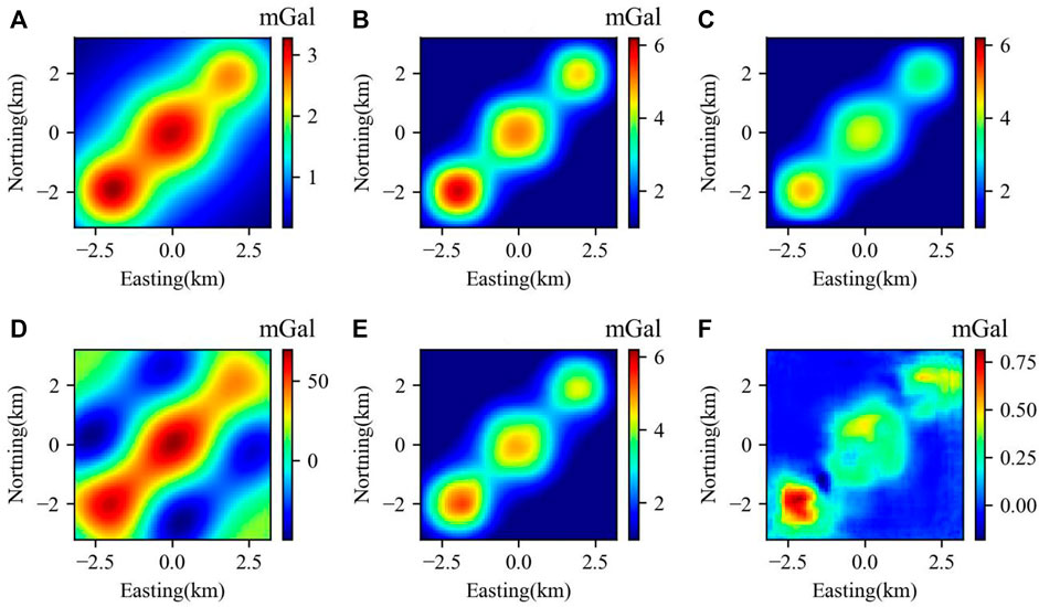
FIGURE 5. DC results for different methods: (A) gravity anomaly at 500 m; (B) true value of the gravity anomaly at 0 m; (C) DC gravity anomaly at 0 m using the TEDC method; (D) DC gravity anomaly at 0 m using the DFDC method with a filter equal to 1000; (E) DC gravity anomaly at 0 m using the DC-Net model; (F) error between (B) and (E).
From the comparison of Figures 5B–E, we observed that the gravity anomaly at 0 m derived from the TEDC method (Figure 5C) is better than that from the DFDC method (Figure 5D), but it is still quite fuzzy in comparison with the true value shown in Figure 5B. In contrast, almost all the high-frequency features of the gravity anomalies are recovered successfully by our DC-Net model (Figure 5F). The gravity anomaly predicted by the DC-Net model (Figure 5E) is more consistent with the true value (Figure 5B) than those obtained by the mainstream methods (Figures 5C, D).
Table 2 shows the different errors between the continuation gravity anomaly results at 0 m altitude (Figures 5C–E) and the true gravity anomaly at the same altitude (Figure 5B). By comparing the different errors in Table 2, we can infer that the continuation high-resolution gravity anomaly at 0 m altitude (Figure 5E) using the CNN model is the most reliable by comparing it with the results of the other two methods (Figures 5B, C). The MSE of the different errors for DC-Net predictions is less than 0.0036 mGal.
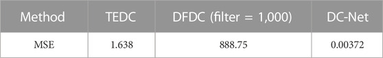
TABLE 2. MSE of errors between the continuation gravity anomaly results and the true gravity anomaly using different methods at 0 m altitude.
This part of the experiment demonstrates that we obtained reliable prediction results, even for data that were not included in the training dataset, which could be explained as follows: during the training process, our network was not only learning a one-to-one analogical connection from the training sets, but also the DC law between them.
3.5 Noise effect
In practice, the observed gravity anomaly is usually severely contaminated by various amounts of high-frequency noise caused by disturbance factors, such as engine vibration, sensor drifts, environmental noise, and irregular operations (Pajot et al., 2008). An obvious problem with traditional DC algorithms is that they are easily affected by high-frequency noise (Tran and Nguyen, 2020). Therefore, it is necessary to test the robustness to noise of our CNN-based model.
To ensure that the test was comprehensive, we trained the model twice under the same CNN framework. We refer to the CNN model applied to noise-free training sets as NFDC-Net and refer to the model applied to training sets with changing levels of noise as DC-Net. In our test, we set noise to a Gaussian stochastic type with the level randomly selected between 0% and 6%. Using the two well-trained models, we conducted eight experiments with four types of low-resolution gravity anomalies contaminated by Gaussian noise with zero mean and with the variances set to 0%, 2%, 5%, and 10% of the maximum amplitude, as shown in Figures 6A–D, respectively. We predicted all the types of gravity data using the NFDC-Net model and the DC-Net model individually. The corresponding prediction results are presented in Figures 6E–L.
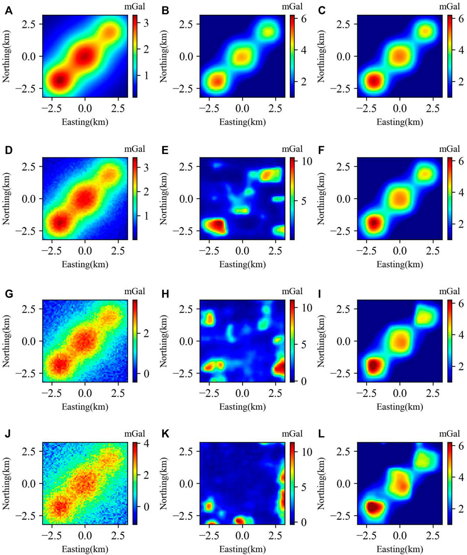
FIGURE 6. Predicted results at 0 m using the NFDC-Net model and the DC-Net model for different gravity anomalies with different noise levels at 500 m: (A) noise-free gravity anomaly; (B) predicted result using the NFDC-Net model for a noise-free gravity anomaly; (C) predicted result using the DC-Net model for a noise-free gravity anomaly; (D) gravity anomaly with 2% Gaussian noise; (E) predicted result using the NFDC-Net model for a gravity anomaly with 2% Gaussian noise; (F) predicted result using the DC-Net model for a gravity anomaly with 2% Gaussian noise; (G) gravity anomaly with 5% Gaussian noise; (H) predicted result using the NFDC-Net model for a gravity anomaly with 5% Gaussian noise; (I) predicted result using the DC-Net model for a gravity anomaly with 5% Gaussian noise; (J) gravity anomaly with 10% Gaussian noise; (K) predicted result using the NFDC-Net model for a gravity anomaly with 10% Gaussian noise; (L) predicted result using the DC-Net model for a gravity anomaly with 10% Gaussian noise.
The results in Figure 6 illustrate that the noise-free trained NFDC-Net model accurately predicted the gravity anomaly without noise (Figure 6E). However, it could not retrieve any useful information from noise-contaminated input data, even when the contamination level was less than 2% (Figures 6F–H). This means that the noise-free trained model failed for the prediction of noisy input. The DC-Net model, which was trained with changing levels of noise, always successfully recovered the high-resolution gravity anomaly at the lower altitude (0 m) both for noise-free input (Figure 6I) and noise-contaminated input (Figures 6I–K). Although the maximum noise level of the DC-Net training sets was 6%, DC-Net still made an effective prediction, even when the input noise was greater than 10%. From these results, we can infer that model training with noise is necessary and that our noise training strategy is effective. Simultaneously, the noise immunity abilities of our CNN-based models can be controlled by the training datasets to a considerable degree.
Table 3 shows the MSE of the errors between the predicted gravity anomaly and true gravity anomaly at 0 m altitude (Figure 5B). By comparing the error results in Table 3, we can see that the predicted near-field gravity anomalies at 0 m altitude using the DC-Net model are more accurate than those predicted by the NFDC-Net model, and the MSE of the different errors for the DC-Net predictions is less than 0.1338 mGal. Consequently, the DC-Net model has the ability to resist noise and is robust.
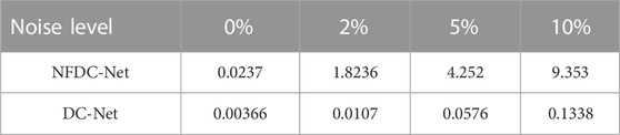
TABLE 3. MSE of errors between the predicted gravity anomaly and the true gravity anomaly at 0 m altitude using different CNN models.
3.6 Multi-times DC
Because we trained our CNN model using only one altitude (500 m), it was difficult for the one-time prediction of our CNN model to satisfy DC requirements with longer continuation distances. Therefore, we implemented repeated continuation tests using the DC-Net model. The test results are shown in Figure 7.
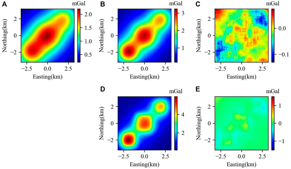
FIGURE 7. Twice DC operation: (A) gravity anomaly at 1,000 m; (B) gravity anomaly at 500 m, calculated by the once DC operation; (C) the error between the predicted gravity anomaly and the true gravity anomaly at 500 m; (D) gravity anomaly at 0 m, calculated by the twice DC operation; (E) error between the predicted gravity anomaly and the true gravity anomaly at 0 m. The true gravity at 500 m is shown in Figure 6A, and the true gravity anomaly at 0 m is shown in Figure 5B.
Figure 7 shows the results and errors of the twice DC operation. First, we calculated the gravity anomaly at 500 m by the once DC operation from the true gravity anomaly at 1,000 m (Figure 7A). The predicted gravity anomaly at 500 m and the error are shown in Figures 7B, C respectively. We then calculated the gravity anomaly at 0 m by another DC operation using the gravity anomaly at 500 m, which was obtained by previous DC operations. The predicted gravity anomaly at 0 m and the error are shown in Figures 7D, E. From the comparison of the predicted gravity anomaly (Figure 7B) and the true value (Figures 6A, 5B) at 500 and 0 m, respectively, we found that the predicted results at different heights are both in good agreement with the true values. However, the predicted error at 500 m, which was obtained by the once DC operation (Figure 7C), is smaller than that at 0 m, which was obtained by the twice DC operation (Figure 7E). The errors could dramatically increase by the accumulation of the DC operation.
This part of the experiment confirmed that our network can be used not only for the continuation distance of 500 m but also longer distances. However, the difference error results (summarized in Table 4) demonstrate an existing accumulative error in the multi-time computation when the continuation distance was increased. It should be noted that a continuation distance that is too long may decrease the prediction accuracy to a certain degree.
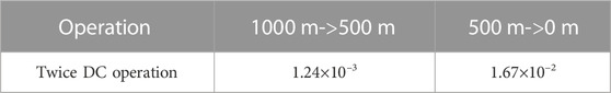
TABLE 4. MSE of errors of repeated DC operations.
4 Application
A test site for AG systems has been established at Kauring, which is approximately 100 km east of Perth, Western Australia. The site was chosen to support AG system tests arranged by the Geological Survey of Western Australia, Geoscience Australia, and Rio Tinto Exploration (Lane et al., 2009). Projects to study different methods to produce terrain correction (Zhdanov and Liu, 2013), to upward continue the ground gravity data (Elieff, 2018), and to separate and interpret vertical gravity data (Liu and Li, 2019) have already commenced.
To verify the validity test of our DC-Net model, we applied the mainstream DC method based on Taylor series expansion (Tran and Nguyen, 2020), which we refer to as the TEDC method, and two CNN-based models (the NFDC-Net model and the DC-Net model) to the gravity anomaly at the Kauring test site at 500 m altitude (Figure 8A). We calculated this gravity anomaly using upward continuation from the observed AG anomaly at the geoid (Figure 8B). We considered the observed gravity anomaly at the geoid as the true value to which the DC predictions should refer.
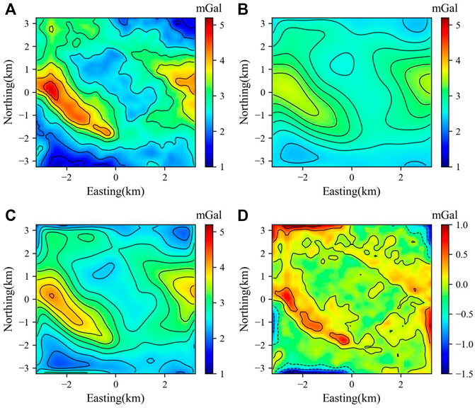
FIGURE 8. (A) Observed gravity anomaly of the Kauring test site at the geoid. (B) Calculated gravity anomaly at 500 m altitude (Blakely, 1996). (C) DC gravity anomaly at 0 m using the Taylor series expansion method (Tran and Nguyen, 2020). (D) Error between (C) and (A).
Figure 8C illustrates the gravity anomaly at the geoid derived from the TEDC method. Figures 9A, C show the gravity anomaly at the geoid predicted by the NFDC-Net model and the DC-Net model, respectively. We then comprehensively compared the continuation results with the true value (Figure 8A). From the comparison of Figures 8A, C, 9A, 9C, we can see that gravity anomalies at the geoid predicted by the NFDC-Net model and the DC-Net model (Figures 9A,C) are more consistent with the true value (Figure 8A) than that obtained by the traditional TEDC method (Figure 8C). The error of the DC gravity anomaly at 0 m based on TEDC method (Figure 8D) is larger than those predicted by the NFDC-Net model and the DC-Net model (Figures 9B,D). The CNN-based models can recover more high-frequency features of the gravity anomaly at the geoid than the TEDC method. This high-frequency anomaly signal is useful for increasing the accuracy of the structural interpretation. Although the actual gravity anomaly data were formed by the superposition of many anomaly bodies, the effectiveness of our two trained models was established.
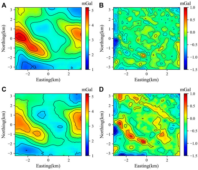
FIGURE 9. (A) Gravity anomaly at the geoid predicted by the NFDC-Net model. (B) Error between (A) and Figure 8A. (C) Gravity anomaly at the geoid predicted by the DC-Net model. (D) Error between (C) and Figure 8A.
Furthermore, the gravity anomaly at the geoid predicted by the NFDC-Net model (Figure 9A) depicted more local partial anomalies than those predicted by the DC-Net model (Figure 9C). The error of the NFDC-Net model prediction (Figure 9B) was smaller than that of DC-Net model prediction (Figure 9D). This may be because during the prediction process using the DC-Net model, certain high-frequency signals were regarded as noise instead of signals. Therefore, in practical applications, we recommend performing noise quantification to constrain the noise level of the training dataset before network training. We expect that this will prevent high-frequency signals from being dropped as unreal noise in real cases.
5 Concluding remarks
In this study, we have proposed DC-Net for the gravity DC problem using DL technology. We introduced the basic theory and critical components of the proposed DC-Net. We performed several synthetic tests and implemented a real application to assess the effectiveness, noise effect, and usability of our DC-Net model. Our main findings are as follows:
(1) The loss function and relative accuracy function curves showed that our network was sufficiently trained. The subset of validation data prediction results showed that a certain number of distinctive boundary and noisy training dataset fed into our DC-Net model ensured that our DC-Net model had a good ability to avoid the Gibbs effect and noise contamination for the DC problem.
(2) We performed DC tests derived from gravity anomaly data that had a different morphological distribution from those in the training dataset using our DC-Net model. The prediction results demonstrated that our DC-Net model learned not only the one-to-one analogical connection from the training sets but also the DC law between them.
(3) DC tests for different gravity anomalies were contaminated with 0%, 2%, 5%, and 10% Gaussian noise successively using different trained models. The prediction results demonstrated that the noise-contaminated trained DC-Net model performed better than the noise-free trained NFDC-Net model. Therefore, noise training is necessary for the DC problem.
(4) The prediction results of repeated DC indicated that our DC-Net model remained valid even for repeated DC. However, there was a cumulative error as the DC distance increased.
(5) The real-world application results demonstrated that the noise-free trained NFDC-Net model predicted more local partial anomalies than the noise-contaminated trained model. Therefore, in a practical scenario, it is necessary to use noise quantification to constrain the noise level of the training dataset. This could prevent high-frequency signals from being dropped as unreal noise.
(6) It is noteworthy that gravity anomalies caused by real geological bodies are not in the training set, but our DC-Net model could still have good DC predictions for real-world data. It may be the case that CNN can provide not only the simple mapping from
Data availability statement
The datasets presented in this study can be found in online repositories. The open-source Python library for the DC-Net model can be downloaded from GitHub (https://github.com/LiYongbo-geo/DCNet-code.git).
Author contributions
HL, SC, YL, BZ, MZ, and JH designed the research plan. HL and YL designed the DC-Net model, conducted the experiments, drew the figures and tables, and wrote the original draft of the manuscript. SC created the concept for the study and supervised the entire study. YL and BZ wrote the program for the CNN. MZ and JH performed validation tests for the program. All authors revised the manuscript and approved the final version for publication validation for the program.
Funding
This work was jointly supported by the National Natural Science Foundation of China (Grant Numbers 42004074 and U1939205) and the Special Fund of the Institute of Geophysics, China Earthquake Administration (Grant Number DQJB22R32, DQJB19A0121, and DQJB22X12).
Acknowledgments
We gratefully acknowledge the researchers, agencies, and companies who established the Kauring test site and made the associated data available. We greatly appreciate the public program about TEDC method sharing by Tran van Kha and Trung Nguyen Nhu. We thank two reviewers SL and DZ, the Editor Prof. SO and assistant Editor for their valuable comments and patience works during the revision process. We thank Jinzhao Liu (The First Monitoring and Application Center, China Earthquake Administration, Tianjin, China) for the helpful discussions of this manuscript and thank Maxine Garcia for editing the English text of a draft of this manuscript.
Conflict of interest
The authors declare that the research was conducted in the absence of any commercial or financial relationships that could be construed as a potential conflict of interest.
Publisher’s note
All claims expressed in this article are solely those of the authors and do not necessarily represent those of their affiliated organizations, or those of the publisher, the editors, and the reviewers. Any product that may be evaluated in this article, or claim that may be made by its manufacturer, is not guaranteed or endorsed by the publisher.
References
Adewumi, T., and Salako, K. (2018). Delineation of mineral potential zone using high resolution aeromagnetic data over part of Nasarawa State, North Central, Nigeria. Egypt. J. Petroleum 27 (4), 759–767. doi:10.1016/j.ejpe.2017.11.002
Alzubaidi, L., Zhang, J., Humaidi, A. J., Al-Dujaili, A., Duan, Y., Al-Shamma, O., et al. (2021). Review of deep learning: Concepts, CNN architectures, challenges, applications, future directions. J. Big Data 8 (1), 53–74. doi:10.1186/s40537-021-00444-8
Bergen, K. J., Johnson, P. A., de Hoop, M. V., and Beroza, G. C. (2019). Machine learning for data-driven discovery in solid Earth geoscience. Science 363 (6433), eaau0323. doi:10.1126/science.aau0323
Blakely, R. J. (1996). Potential theory in gravity and magnetic applications. Cambridge, UK: Cambridge University Press.
Branchaud-Charron, F., Achkar, A., and Jodoin, P. M. (2019). “Spectral metric for dataset complexity assessment,” in Proceedings of the IEEE/CVF conference on computer vision and pattern recognition, Long Beach, CA, USA, 3215–3224, doi:10.1109/CVPR.2019.00333
Chen, M., and Yang, W. (2022). An enhancing precision method for downward continuation of gravity anomalies. J. Appl. Geophys. 204, 104753. doi:10.1016/j.jappgeo.2022.104753
Cooper, G. (2004). The stable downward continuation of potential field data. Explor. Geophys. 35 (4), 260–265. doi:10.1071/eg04260
Cordell, L., and Grauch, V. (1985). “Mapping basement magnetization zones from aeromagnetic data in the San Juan Basin, New Mexico,” in The utility of regional gravity and magnetic anomaly maps. Society of Exploration Geophysicists, Houston, TX 181–197.
Elieff, S. (2018). The interplay of sampling and accuracy in gravity surveys, New Orleans, AK, USA: SEG International Exposition and Annual Meeting.
Geng, Z., Wu, X., Shi, Y., and Fomel, S. (2020). Deep learning for relative geologic time and seismic horizons. Geophysics 85 (4), WA87–WA100. doi:10.1190/geo2019-0252.1
Ghodrati, V., Shao, J., Bydder, M., Zhou, Z., Yin, W., Nguyen, K-L., et al. (2019). MR image reconstruction using deep learning: Evaluation of network structure and loss functions. Quantitative Imaging Med. Surg. 9 (9), 1516–1527. doi:10.21037/qims.2019.08.10
Halpert, A. D. (2018). Deep learning-enabled seismic image enhancement. Houston, TX: SEG Technical Program Expanded Abstracts 2018 Society of Exploration Geophysicists, 2081–2085.
Han, B., Hu, Z., Su, Z., Bai, X., Yin, S., Luo, J., et al. (2022). Mask_LaC R-CNN for measuring morphological features of fish. Measurement 203, 111859. doi:10.1016/j.measurement.2022.111859
Lane, R., Grujic, M., Aravanis, T., Tracey, R., Dransfield, M., Howard, D., et al. (2009). The Kauring airborne gravity test site, western Australia. San Francisco, CA, USA: AGU Fall Meeting Abstracts.
Liu, D-J., Hong, T-Q., Jia, Z-H., Li, J-S., Lu, S-M., Sun, X-F., et al. (2009). Wave number domain iteration method for downward continuation of potential fields and its convergence. Chin. J. Geophys. 52 (6), 1599–1605. doi:10.3969/j.issn.0001-5733.2009.06.022
Liu, J. Z., and Li, H. L. (2019). Separation and interpretation of gravity field data based on two dimensional normal space-scale transform (NSST2D) algorithm: A case study of Kauring airborne gravity test site, western Australia. Pure Appl. Geophys. 176 (6), 2513–2528. doi:10.1007/s00024-019-02131-5
Luo, Y., and Wu, M-P. (2016). Minimum curvature method for downward continuation of potential field data. Chin. J. Geophys. 59 (1), 240–251. doi:10.6038/cjg20160120
Ma, G., Liu, C., Huang, D., and Li, L. (2013). A stable iterative downward continuation of potential field data. J. Appl. Geophys. 98, 205–211. doi:10.1016/j.jappgeo.2013.08.018
Mao, X., Li, Q., Xie, H., Lau, R. Y., Wang, Z., and Paul Smolley, S. (2017). “Least squares generative adversarial networks,” in Proceedings 2017 IEEE International Conference on Computer Vision (ICCV), Venice, Italy, doi:10.1109/ICCV.2017.304
Nagy, D., Papp, G., and Benedek, J. (2000). The gravitational potential and its derivatives for the prism. J. Geodesy 74 (7), 552–560. doi:10.1007/s001900000116
Pajot, G., De Viron, O., Diament, M., Lequentrec-Lalancette, M-F., and Mikhailov, V. (2008). Noise reduction through joint processing of gravity and gravity gradient data. Geophysics 73 (3), I23–I34. doi:10.1190/1.2905222
Pašteka, R., Karcol, R., Kušnirák, D., and Mojzeš, A. (2012). Regcont: A MATLAB based program for stable downward continuation of geophysical potential fields using Tikhonov regularization. Comput. Geosciences 49, 278–289. doi:10.1016/j.cageo.2012.06.010
Peters, L. J. (1949). The direct approach to magnetic interpretation and its practical application. Geophysics 14 (3), 290–320. doi:10.1190/1.1437537
Ronneberger, O., Fischer, P., and Brox, T. (2015). “U-net: Convolutional networks for biomedical image segmentation,” in International Conference on Medical image computing and computer-assisted intervention (Manhattan, NY, USA: Springer Cham), 234–241.
Tai, Z., Zhang, F., Zhang, F., and Hao, M. (2016). Approximate iterative operator method for potential-field downward continuation. J. Appl. Geophys. 128, 31–40. doi:10.1016/j.jappgeo.2016.03.021
Tran, K. V., and Nguyen, T. N. (2020). A novel method for computing the vertical gradients of the potential field: Application to downward continuation. Geophys. J. Int. 220 (2), 1316–1329. doi:10.1093/gji/ggz524
Wang, E., and Nealon, J. (2019). Applying machine learning to 3D seismic image denoising and enhancement. Interpretation 7 (3), SE131–SE139. doi:10.1190/int-2018-0224.1
Wang, Y., Zhang, Y., Fu, L., and Li, H. (2021). Three-dimensional gravity inversion based on 3D U-Net++. Appl. Geophys. 18 (4), 451–460. doi:10.1007/s11770-021-0909-z
Yang, F., and Ma, J. (2019). Deep-learning inversion: A next-generation seismic velocity model building method. Geophysics 84 (4), R583–R599. doi:10.1190/geo2018-0249.1
Yu, S., Ma, J., and Wang, W. (2019). Deep learning for denoising. Geophysics 84 (6), V333–V350. doi:10.1190/geo2018-0668.1
Zeng, X-N., Li, X-H., Han, S-Q., and Liu, D-Z. (2011). A comparison of three iteration methods for downward continuation of potential fields. Prog. Geophys. 26 (3), 908–915. doi:10.3969/j.issn.1004-2903.2011.03.016
Zhang, H., Chen, L. W., Ren, Z. X., Wu, M. P., Luo, S. T., and Xu, S. Z. (2009). Analysis on convergence of iteration method for potential fields downward continuation and research on robust downward continuation method. Chin. J. Geophys. 52 (2), 511–518. doi:10.1002/cjg2.1371
Zhang, H., Yang, X., and Ma, J. (2020). Can learning from natural image denoising be used for seismic data interpolation? Geophysics 85 (4), WA115–WA136. doi:10.1190/geo2019-0243.1
Zhang, Z., Yu, P., Zhang, L., Zhao, C., Wang, Y., and Xu, Y. (2021). Application of U-net for the recognition of regional features in geophysical inversion results. IEEE Trans. Geoscience Remote Sens. 60, 1–7. doi:10.1109/tgrs.2021.3138790
Zhao, M., Chen, S., and Yuen, D. (2019). Waveform classification and seismic recognition by convolution neural network. Chin. J. Geophys. 62 (1), 374–382. doi:10.6038/cjg2019M0151
Zhdanov, M. S., and Liu, X. (2013). 3-D Cauchy-type integrals for terrain correction of gravity and gravity gradiometry data. Geophys. J. Int. 194 (1), 249–268. doi:10.1093/gji/ggt120
Zhou, W., Zhang, C., and Zhang, D. (2022). A novel downward continuation method based on continued fraction in wavenumber domain and its application on aeromagnetic data in the Xuanhua-Huailai area, China. Pure Appl. Geophys. 179 (2), 777–793. doi:10.1007/s00024-021-02937-2
Keywords: gravity downward continuation, convolutional neural network, deep learning, upscaling low-resolution images, DC-Net model
Citation: Li H, Chen S, Li Y, Zhang B, Zhao M and Han J (2023) Stable downward continuation of the gravity potential field implemented using deep learning. Front. Earth Sci. 10:1065252. doi: 10.3389/feart.2022.1065252
Received: 09 October 2022; Accepted: 08 December 2022;
Published: 09 January 2023.
Edited by:
Saulo Oliveira, Federal University of Paraná, BrazilReviewed by:
Shuang Liu, China University of GeosciencesWuhan, ChinaDailei Zhang, Chinese Academy of GeologicalScience, China
Copyright © 2023 Li, Chen, Li, Zhang, Zhao and Han. This is an open-access article distributed under the terms of the Creative Commons Attribution License (CC BY). The use, distribution or reproduction in other forums is permitted, provided the original author(s) and the copyright owner(s) are credited and that the original publication in this journal is cited, in accordance with accepted academic practice. No use, distribution or reproduction is permitted which does not comply with these terms.
*Correspondence: Shi Chen, Y2hlbnNoaUBjZWEtaWdwLmFjLmNu