 Balazs Markus
 Sébastien Valade
 Manuel Wöllhaf
 Olaf Hellwich1
94% of researchers rate our articles as excellent or good
Learn more about the work of our research integrity team to safeguard the quality of each article we publish.
Find out more
ORIGINAL RESEARCH article
Front. Earth Sci., 05 January 2023
Sec. Volcanology
Volume 10 - 2022 | https://doi.org/10.3389/feart.2022.1064171
This article is part of the Research TopicRemote Sensing of Volcanic Gas Emissions from the Ground, Air, and SpaceView all 18 articles
Volcanic sulfur dioxide (SO2) satellite observations are key for monitoring volcanic activity, and for mitigation of the associated risks on both human health and aviation safety. Automatic analysis of this data source, including robust source emission retrieval, is in turn essential for near real-time monitoring applications. We have developed fast and accurate SO2 plume classifier and segmentation algorithms using classic clustering, segmentation and image processing techniques. These algorithms, applied to measurements from the TROPOMI instrument onboard the Sentinel-5 Precursor platform, can help in the accurate source estimation of volcanic SO2 plumes originating from various volcanoes. In this paper, we demonstrate the ability of different pixel classification methodologies to retrieve SO2 source emission with a good accuracy. We compare the algorithms, their strengths and shortcomings, and present plume classification results for various active volcanoes throughout the year 2021, including examples from Etna (Italy), Sangay and Reventador (Ecuador), Sabancaya and Ubinas (Peru), Scheveluch and Klyuchevskoy (Russia), as well as Ibu and Dukono (Indonesia). The developed algorithms, shared as open-source code, contribute to improving analysis and monitoring of volcanic emissions from space.
The accurate retrieval of the source location and mass loading of volcanic plumes is essential to study volcanic processes and mitigate the associated hazards. In particular, Sulfur Dioxide (SO2) gas emissions are a key parameter informing on the eruptive activity of volcanoes (Oppenheimer et al., 2014). An increase in SO2 flux is for instance often considered as a precursor to volcanic eruptions. Likewise, decrease in SO2 emissions can indicate changes in the volcanic conduit permeability (Edmonds et al., 2003), which can lead to violent explosions (Matthews et al., 1997; Campion et al., 2018). Moreover, these volcanic gases can have severe impact on human health (Sierra-Vargas et al., 2018; Carlsen et al., 2021; Heaviside et al., 2021 and air traffic safety Bernard and Rose, 1990; Prata, 2009; Schmidt et al., 2014). In particular, injection of sulfur dioxide in the atmosphere receives considerable attention due to its subsequent conversion into aerosols and potentially strong effects on global climate (Robock, 2000).
Space-based measurements of the atmospheric composition have blossomed over the past 2 decades, from relatively crude, prototype products, to refined products suitable for operational monitoring and assimilation. These products include tropospheric vertical column density of different gases, including SO2 (Carn et al., 2017). In 2017, the Tropospheric Monitoring Instrument (TROPOMI) was launched onboard the Sentinel-5 Precursor satellite. Thanks to an improved spatial resolution at nadir (i.e., 3.5 km × 7 to 5.5 km footprint) and a better SO2 detection limit (by a factor of 4 with respect to previous sensors), it significantly improved the possibility of detecting small SO2 volcanic emissions previously undetectable (Theys et al., 2017; Theys et al., 2019). In turn, TROPOMI has been extensively used to accurately measure SO2 masses and fluxes emitted from both passive volcanic degassing and large explosive eruptions (Corradini et al., 2021; Queißer et al., 2019; Pardini et al., 2020).
Nonetheless, the SO2-contaminated pixels have no data regarding their origin nor source emission, meaning that only manual inspection and interpretation by the user can determine this. Yet it is of primordial importance to be able to discriminate gas plumes originating from neighboring volcanoes, especially in locations where multiple volcanoes are located in a relatively small area. Various attempts have been made to automatically obtain mass of SO2 emitted from active volcanoes. The MOUNTS operational volcano monitoring system (Valade et al., 2019) for example, which automatically processes TROPOMI products over several tens of active volcanoes worldwide, was using in its initial version a radius-based approach to obtain SO2 mass values per volcano, whereby SO2 contaminated pixels were classified based on their distance to the source volcano. This method however presents pitfalls as gas emissions coming from neighboring volcanoes cannot be discriminated in a robust manner.
In general, SO2 source emission estimation is most often performed manually, which is a tedious process involving human work. Automating this process can make analysis of eruptions significantly faster and more accurate, with the ultimate goal to provide the derived information in near real-time. Automatic plume detection algorithms for TROPOMI products have been actively researched in the recent years, not just for SO2 (Cofano et al., 2021), but also for other gas species recorded by TROPOMI such as NO2 (Finch et al., 2022). This work focuses on the retrieval of the gas source emission, rather than on its detection in the TROPOMI product.
We present different algorithms that were developed to retrieve the source of volcanic SO2-contaminated pixels. The efficiency of these algorithms is tested at various active volcanoes worldwide. The article is organized as follows: in Section 2, the used materials and data are presented. In Section 3, the methods developed to classify the source of SO2-contaminated pixels are summarized. The shortcomings, strengths and the overall results are presented in Section 4 while in Section 5 a discussion of the results and areas of improvement are presented. Final conclusions are then drawn in Section 6.
In this work, Sentinel-5P Near-Real-Time (NRTI) L2 SO2 products were used. NRTI products are suited for near-real-time applications and are only available during 15-days after sensing, after which they are merged and replaced by Offline (OFFL) products. For an arbitrary pixel in the product, several relevant data is available, including: vertical column density (VCD), which correspond to SO2 gas density computed over vertical slices (1 km thick slices at three different altitudes of the atmosphere), the latitude and longitude of the pixel center point, and a SO2 detection flag, provided in the TROPOMI SO2 L2 product as “sulfurdioxide_detection_flag”. This flag identifies pixels with a high SO2 concentration (Romahn et al., 2022), by marking them with either 0 for no detection, 1 for SO2 detection, 2 for clear volcanic detection, 3 for detection close to a known anthropogenic source, or 4 for detection at high SZA (potential false-positive). We hereafter use the term “detection mask” to refer to the matrix of all SO2-contaminated pixels (all the pixels marked with flag ≥1), which is used as input to the algorithms presented here. Summing up the pixels volcanic SO2 detection mask, using the vertical column density (VCD), the total mass of volcanic SO2 plumes on the image can be calculated (Valade et al., 2019). This total SO2 mass can then be assigned to one or multiple source volcanoes.
The algorithms were evaluated on non-cropped L2 SO2 NRTI products collected by the monitoring system MOUNTS (http://www.mounts-project.com, Valade et al., 2019) over seven active volcanoes. These include: Sangay, Sabancaya, Nevado del Ruiz, Etna, Popocatépetl, Dukono, and Yasur, as shown in Table 3. These volcanoes were chosen based on their sustained SO2 degassing activity, and based on the fact that several are located in regions where other nearby volcanoes are emitting contemporaneously. This allowed us to test the algorithms capability to discriminate plumes originating from different neighboring volcanoes. It is worth specifying that these volcanoes are those used for the quantitative evaluation of the algorithms, which implied generating hand-labeled ground truth (see Section 2.2). The algorithms were then applied to a larger list of volcanoes for qualitative evaluation, some of which are presented in the paper (e.g., Scheveluch, Klyuchevskoy, Ibu, Ubinas, Reventador). The products used for evaluation were acquired during the year 2021. In order to decrease the overall dataset, we selected 1 TROPOMI acquisition per day and per volcano, with 10-day interval between the products, resulting in a total of 231 non-cropped TROPOMI products used for evaluation. Given that the satellite orbit cycle repeat time is 16 days, this 10-day sampling allowed to sample various swath positions for each volcano, while reducing the overall dataset size.
In order to evaluate the performances of the algorithms, the entire set of volcanic SO2 detection masks was hand-labeled with a unique label according to the source volcano, which was manually determined based on available meteorological data and volcano eruption records. These manual labels form the “ground truth”, which is compared with the automated classification results to obtain metrics of their efficiency. The ground truth has the same size as the SO2 detection mask, but instead of detection flags it contains either the source volcano ID for each flagged pixel, or a label of false volcanic SO2 detection (which may occur when SO2 pixels from anthropological sources get detected by the sensor as a volcanic SO2 pixel–in this case the pixel should not be assigned to any volcano).
The algorithms use a list of volcano-specific data, which consists of the latitude, longitude, elevation, and a unique identification number for several volcanoes. In this list, all the volcanoes from the MOUNTS monitoring system (Valade et al., 2019) are included, even those that are not present in our case study, as they play a role in the way how some of the presented algorithms work.
In order to obtain estimated trajectories of SO2 plumes, the Hybrid Single-Particle Lagrangian Integrated Trajectory model (HYSPLIT) is used. HYSPLIT is a numerical model that is used to compute air parcel trajectories to determine how far and in what direction a parcel of air, and subsequently air pollutants, will travel. Lagrangian particle models compute trajectories of a large number of so-called particles to describe the transport and diffusion of tracers in the atmosphere (Stein et al., 2015). Combined with the archived reprocessed GDAS meteorological models (NCEP, NWS, NOAA, U.S. DOC, 2009), which are publicly available on NOAA’s FTP servers, the estimated latitude and longitude of an air parcel can be obtained along a specified time range with great temporal resolution (Warner, 2018). Although reprocessed GDAS models are less suited to near real-time applications than the forecast GDAS models, these are expected to perform significantly better. The presented plume trajectories used by the algorithms were computed on a 12-h time range before/after sensing with 1-h temporal resolution. When generating forward trajectories, the start time of the trajectory is set to 1 h before the image acquisition time, and the backwards trajectories are started exactly at the image acquisition time.
The goal is, using the input of non-classified pixels of the volcanic SO2 detection map (as non-geocoded matrices), and the additional wind and volcano information, to obtain an output of classified pixels, which can provide information about which volcano each pixel originates from. One volcano represents a class, meaning that a pixel being classified to a volcano can be interpreted as saying that the pixel originates from that specific volcano.
To reach this goal, eight algorithms are presented, as depicted in Table 1, in ascending order of complexity. Two approaches are tested, as shown in Figure 1: the first corresponds to binary classification methods (BC), which can decide whether a pixel is originating from a selected volcano (the queried volcano is required as an input) or not, and the second corresponds to multi-class classification methods (MC), which provide an estimate for each pixel about which volcano it originates from (no input volcano required). In the final subsection, the metrics used for the evaluation of these algorithms are presented.
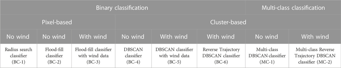
TABLE 1. Overview of all the tested methods.
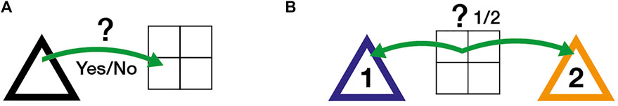
FIGURE 1. Difference between binary and multi-class classification approaches. (A) Binary approach. (B) Multi-class approach.
An intuitive approach is to select a volcano, and iterate through the pixels with a binary decision algorithm that either associates the pixel with the selected volcano, or leaves it unassociated. Six binary-class classification algorithms are tested, which we describe hereafter.
The radius search classifier automatically associates every SO2 detection within a specified arbitrary radius (100 km by default in this paper). The algorithm starts from the pixel at volcano center, then it iteratively jumps onto the next nearest unassociated pixel, as shown in Figure 2A. The distance of the pixel is then calculated with Vincenty’s formulae using the ellipsoidal model WGS-84, which provides better accuracy than a plain spherical model (Vincenty, 1975). This process continues until the calculated distance of the new pixel is above the specified radius.
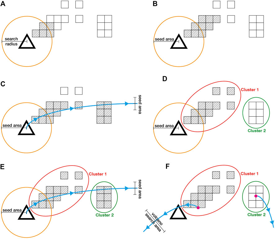
FIGURE 2. Demonstration of the binary classifier algorithms. (A) Radius search classifier. (B) Flood-fill classifier. (C) Flood-fill classifier with wind data. (D) DBSCAN classifier. (E) DBSCAN classifier with wind data. (F) Reverse Trajectory DBSCAN classifier.
Flood-fill is a standard algorithm used to identify and change adjacent values in a multidimensional array, based on their similarity to an initial seed point. The conceptual analogy is the “paint bucket” tool in many graphic editors. The Flood-fill algorithm can be simply modeled as a graph traversal problem, representing the given area as a matrix and considering every cell of that matrix as a vertex that is connected to points around it. The seed point for the algorithm is set by default to the pixel where the volcano of interest is located. As the goal of the algorithm is to classify pixels that are flagged with detected SO2-contamination, the seed point has to be an SO2-flagged one on the detection mask (then, pixels marked with flag ≥1 that are touching the seed point are classified, and the filling continues until there are no additional touching points). If the seed point above the volcano is zero (meaning that there is no flagged SO2 contamination), the algorithm searches for the nearest non-zero element within the seed area (20 km chosen by default in this paper), and if it finds one, it becomes the seed point, as shown in Figure 2B.
With the Flood-fill classifier (BC-2), the algorithm could only have one seed point. This case further increases the number of seed points via an extension where a predicted plume trajectory is generated, starting from the top of the queried volcano. Every point on this trajectory acts as a seed point, and if the trajectory point on the SO2 detection mask is zero, the algorithm searches for the nearest non-zero element in a seed area the same way as with the original seed point, as shown in Figure 2C.
In the three previous algorithms, classification is done on a pixel level, using only information that is available for that individual pixel (i.e., values of pixels within the locality of another pixel are ignored). With object-based classification, the algorithms are working on a localized group of pixels, taking the spatial properties of each pixel and their relationship to each other into account. In this sense, an example for a classification algorithm acts on of a group of pixels, and the classification algorithm would accordingly output a class prediction for pixels on a group basis.
In order to acquire clusters, the DBSCAN (Density-based spatial clustering of applications with noise) algorithm is used. Based on a set of points, DBSCAN can group together points that are close to each other based on a (usually Euclidean) distance measurement and a minimum number of points (Ester et al., 1996). Furthermore, it is also capable of marking points in low-density regions as outliers.
Similarly to the Flood-fill classifier (BC-2), the DBSCAN classifier (BC-4) starts from a seed point and assigns new pixels to the cluster in an iterative way, with the difference that it is not filling pixels one-by-one, but rather whole clusters of pixels, as shown in Figure 2D. The seed area, similarly to the Flood-fill algorithms, is the pixel at the center of the volcano and its near area (20 km chosen by default in this paper).
The algorithm generally requires two parameters. The first is the parameter ɛ, which specifies how close points should be to each other on a pixel grid to be considered a part of a cluster. If the grid distance between two points is lower or equal to this value, those two points are considered neighbors. The second parameter is called minPoints, and it represents the minimum number of points to form a dense region. For example, setting the minPoints parameter as 4 means that at least 4 points are needed to form a dense region. Setting the ɛ parameter low generally produces more clusters, but it also results in an increased number of outliers, as shown in Figure 3. We chose a value ɛ = 4.0 and minPoints = 3 for our use case, which gave best results when applied to the TROPOMI data set. These values were chosen manually by testing several products, where noise points and outliers were minimized while preserving as many clusters as possible. In addition, DBSCAN makes it possible to assign weights to each pixel. We used the SO2 column density value of each pixel as weights when creating clusters. This improves clustering in cases when multiple plumes originating from neighboring volcanoes come to overlap. In such a case they are forming a common plume, but as the SO2 density generally tends to be higher around the center of the source volcanoes, the distinct high-density areas (which are thus highly weighted) can induce a separation of the unique plume into smaller clusters.
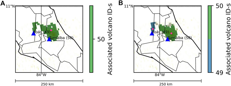
FIGURE 3. Difference in the created DBSCAN clusters with touching plumes (Turrialba and Poás volcanoes, on 23.03.2021), depending on the ɛ value. (A) ɛ = 4.0 (B) ɛ = 1.0.
Similarly to the Flood-fill classifier with wind data (BC-3), this case is an extension of the DBSCAN classifier where a predicted plume trajectory is generated, starting from the top of the queried volcano, as shown in Figure 2E. Every point of this trajectory acts as a seed point, and if the trajectory point on the SO2 detection mask is zero, the algorithm searches for the nearest non-zero element in a seed area the same way as with the original seed point.
A reverse plume trajectory is started from the center of mass of each cluster using the wind models, as shown in Figure 2F. The position of the center of mass is computed in grid space (i.e., in the non-geocoded matrix), weighted by the VCD values (raised to the power of 4 to make the dense parts more dominant in the positioning of the reference point in long plumes, as opposed to the simple DBSCAN classifier, where the weights only serve the cluster generation), and the latitude and longitude of the corresponding pixel is then used to define the cluster position, from which the trajectory is started. On the other hand, the altitude from which the trajectory is computed is defined as the summit altitude of the queried volcano. If a trajectory that was started from a plume is within a specified distance of the queried volcano (50 km by default in this paper), the cluster is associated with it. In the ideal case, the trajectory that starts from a cluster that is actually originating from the queried volcano should go right over the volcano.
The aforementioned algorithms have a common shortcoming: when applied to a TROPOMI product that covers an area that contains multiple volcanoes (which happens frequently in areas with high volcano density), the iterative use of binary classifiers can result in ambiguous, overlapping classifications, as shown in Figure 4. For example, if the predicted plume trajectories of two different volcanoes intersect, i.e. contain the same pixels, those pixels are going to be associated with both volcanoes. This happens frequently with nearby volcanoes (e.g., Ibu and Dukono volcanoes, only 35 km apart from one another). To prevent that, the algorithms should be retrofitted based on the fundamental concept that a pixel can only be associated with one volcano.

FIGURE 4. Iterative use of binary classifiers on the same image can result in overlapping classifications.
The binary DBSCAN classifier algorithm could only associate one cluster to a volcano, even though it is possible for multiple clusters to originate from one source. To eliminate this problem, first we build the clusters the same way as we did in the binary DBSCAN case (BC-4), then we decide whether a cluster is going to be associated or not. This algorithm does not use any wind models, it only relies on the location of the volcanoes and the generated clusters (see Algorithm 1 pseudo-code). The latitude and longitude position of a cluster are equal to its calculated center of mass (computed in grid space, as described in BC-6), and the distance to the volcano is computed as the geodetic distance to the volcano summit. The plume height does not play a role in this case.
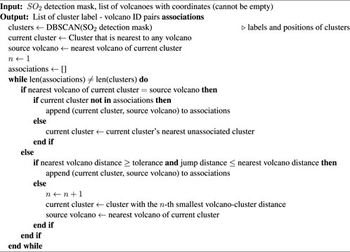
ALGORITHM 1. Multi-class DBSCAN classifier algorithm (MC-1).
First, the cluster that is the nearest to any volcano on the image is selected as a starting cluster, and its nearest volcano becomes the “source volcano”. The algorithm associates the nearest unassociated clusters until the new cluster’s nearest volcano is not the source volcano anymore - in that case, it checks how far the new cluster is from the nearest volcano. If it’s above a specified tolerance (200 km by default in this paper), and the new cluster is closer to the previous cluster than to the nearest volcano, it keeps assigning it to the original source volcano. This is to prevent another volcano of “hijacking” a plume in long stretched plume groups, when the plume is already closer to another cluster than to the original source volcano. Without this addition, the algorithm would associate every cluster automatically to the closest volcano. The procedure is depicted in Figure 5A.
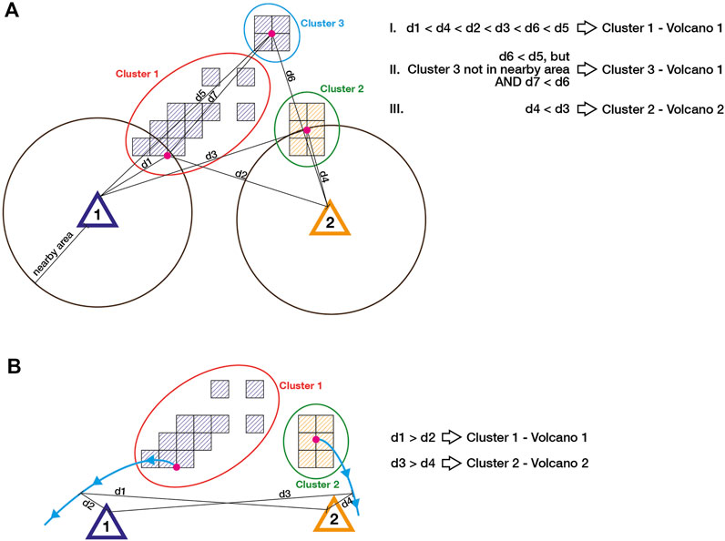
FIGURE 5. Demonstration of the multi-class algorithms. The magenta dot represents the plume center of mass, and the colored ovals show the generated clusters. (A) Multi-class DBSCAN classifier. (B) Multi-class Reverse Trajectory DBSCAN classifier.
If the aforementioned conditions do not apply, meaning that the next nearest cluster is farther than the specified tolerance (200 km), or if it is closer to its nearest volcano than to the previous cluster, the algorithm stops assigning clusters to the original source volcano, and it selects a new source volcano to start from. This is the volcano that is the nearest to any unassociated cluster (similarly, at the beginning we started at the smallest volcano-unassociated cluster distance, but at that time all the clusters were unassociated). The clusters are then being assigned the same way as with the original source volcano. To keep track of the jumps (and to be able to select the new source volcano), the number of source volcano changes is stored. Optionally, clusters that are further away from volcanoes and other clusters than a specified tolerance can be left unclassified. This is to ignore occasional false positives in the volcanic SO2 detection mask in the TROPOMI product.
This algorithm follows the same logic as the binary Reverse Trajectory DBSCAN classifier (BC-6), with the additional rule that every cluster has to be associated with only one volcano (see Algorithm 2 pseudo-code). A reverse plume trajectory is started from the center of mass of every cluster using the wind models, as shown in Figure 5B. The latitude and longitude position of a cluster are equal to its center of mass, and the height of the plume, where the trajectory is started from, is equal to the elevation of its nearest volcano. As the TROPOMI L2 SO2 product does not include plume height, using an input volcano’s elevation as a plume height would make the algorithm volcano-dependent, and with this solution we can overcome that problem. The cluster is associated with the volcano that is nearest to any point of the reverse trajectory. In the ideal case, the trajectory goes right over the source volcano, which makes this distance zero.
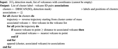
ALGORITHM 2. Multi-class Reverse Trajectory DBSCAN classifier algorithm (MC-2).
Evaluation of classification methods can be quite complex because it is required to measure classification accuracy as well as localization correctness. The aim is to score the similarity between the predicted and annotated volcanoes (prediction vs. ground truth). Over the years, a large variety of evaluation metrics has been introduced. The presented metrics in this work are common, widespread scores for performance measurement in computer vision and remote sensing fields. The main goal in metric selection was to minimize statistical bias in evaluation.
All presented metrics are based on the computation of a confusion matrix for a binary segmentation task, which contains the number of true positive (TP), false positive (FP), true negative (TN), and false negative (FN) predictions. In this context, a true positive pixel is a detected SO2-contaminated pixel which was correctly classified to the queried volcano, and a false positive pixel is one that was incorrectly classified to the queried volcano. Similarly, a true negative pixel is one that is correctly not classified to the queried volcano, and a false negative pixel is one that is incorrectly not classified to the queried volcano. Generally, the value ranges of all presented metrics span from zero (worst) to one (best). The selected metrics are Accuracy, Precision, Recall, and the F1-Score, as presented in Table 2.
• Accuracy represents the fraction of predictions that the evaluated model got right.
• Precision shows the proportion of positive identifications that were actually correct.
• Recall shows the proportion of actual positives that were identified correctly.
• The F1-score is an overall measure of a model’s effectiveness that combines precision and recall, by calculating the harmonic mean. We use the harmonic mean instead of a simple average because it punishes extreme values. A classifier with a precision of 1.0 and a recall of 0.0 has a simple average of 0.5 but an F1-score of 0. That is, a good F1-score means that we have low false positives and low false negatives, so we are correctly identifying real threats and we are not disturbed by false alarms. The aforementioned features make this metric well suited for measuring the performance of the tested algorithms.
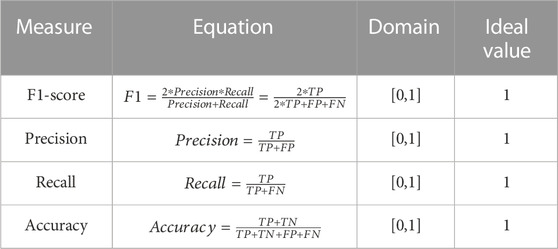
TABLE 2. The performance metrics used in the evaluation.
In this section, the performances of the proposed algorithms are compared using the presented metrics. The algorithms were all implemented in a Python environment. The source code of the algorithms is publicly available from a GitHub repository (Markus, 2022a).
To verify that the accuracy improvement provided by the proposed methods is significant, and to systematically evaluate the performance of the proposed methods we conduct an averaging of the results for different products. We select TROPOMI SO2 products of seven volcanoes, with a 10-day temporal resolution across the year of 2021, as shown in Table 3. The labeled ground truth and the configuration files are publicly available (Markus, 2022b). We compute the accuracy, precision, recall and F1-score for the presented algorithms using the selected products within the specified time range. The values are then averaged for the cases where classification is possible (empty cases without detection are not taken into account). The initial hypothesis is that the multi-class methods reach a higher overall mean accuracy.
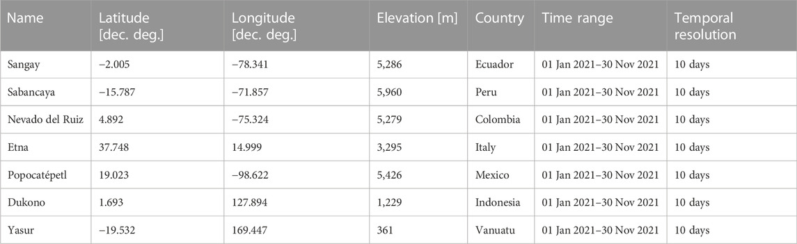
TABLE 3. Contents of the evaluating dataset.
Figure 6 shows a series of TROPOMI SO2 images, overlaid with the classification results of the 8 algorithms described previously. Three cases were considered: Sangay (queried volcano) vs. Reventador 2021-08-15 acquisition, Ubinas (queried volcano) vs. Sabancaya 2021-04-27 acquisition where a plume originating from Sabancaya traveled over the Ubinas volcano, and Sheveluch (queried volcano) vs. Kluchevskoy 2021-03-19 acquisition. Each row in Figure 6 shows the result of a given algorithm for all three cases. The shades of white to yellow/red represent the SO2 gas concentration, the gray pixels are the flagged SO2 detections in the TROPOMI product, and the green/blue filled pixels are the pixels that were associated with a volcano label according to the color bar. The cyan lines are the wind trajectories, and the magenta points represent the center of mass of a generated cluster.
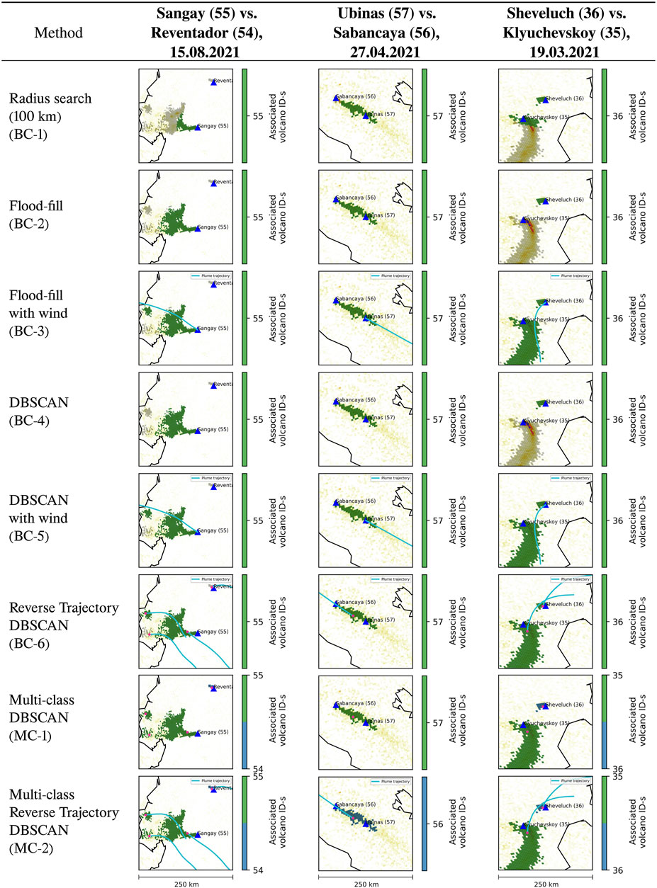
FIGURE 6. Plots of evaluation runs with different classifier algorithms on three volcanic scenarios. The plots represent 250 × 250 km regions. Magenta dots represent cluster center of mass, and cyan lines are computed plume trajectories.
The results for each metric respective to the algorithms are presented in Table 4. Results show that on average, the radius search algorithm (BC-1) under-performs compared to other methods. The precision of the algorithm is high, but the recall value is comparatively low. The small value of recall indicates that this algorithm is prone to under-segmentation (which means it ignores pixels that should have been associated with the volcano), while also not providing any prevention from falsely associating SO2 pixels of nearby volcanoes. This algorithm performs best in areas where the spatial density of volcanoes is low, and/or where winds are low (i.e., plume stays close to the volcano).
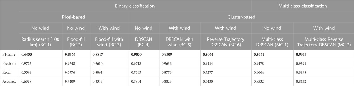
TABLE 4. The mean values of performance metrics across the evaluating dataset.
The second proposed method, Flood-fill (BC-2) shows a higher degree of robustness with respect to the accuracy, and is able to classify entire plumes, which the radius search algorithm failed to achieve (see Figure 7). Still, it fails to provide fully satisfactory classification as it is only able to fill interconnected plumes. Indeed, SO2 plumes often appear discontinuous in TROPOMI imagery, thus making the filling approach incapable of classifying the gas plume as a whole. Small isolated SO2-contaminated pixels near the plume are also left unfilled, as there is no direct connection to the plume. The extension of the Flood-fill algorithm with the air parcel trajectory (BC-3) starting from the volcano achieves a better accuracy, because it is able to fill disconnected plumes, thanks to the wind trajectory which acts as an extended seed area. Although it still leaves isolated SO2 pixels near the main plume unfilled, the bulk of the plume can be successfully filled. Extension of the seed area induces a significant increase in recall, but a small decrease in precision can be observed. Informally, besides reducing under-segmentation, the larger seed area caused the algorithm to incorrectly associate pixels that were originating from a different source, especially in areas of multiple SO2 sources.
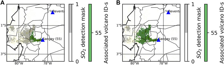
FIGURE 7. Comparison of two basic binary classifications (Sangay volcano, on 15.08.2021). (A) Radius search classifier. (B) Flood-fill classifier.
The cluster-based DBSCAN filling method (BC-4) demonstrates higher accuracy and recall value with respect to the pixel-based Flood-fill, as besides incorporating small isolated SO2 pixels near the edges a plume, fragmented but cohesive plumes are considered as one entity. Extending this with the air parcel trajectory starting from the volcano (BC-5) eliminates the under-segmentation problem when multiple plumes are originating from one volcano, as shown in Figure 8, increasing the recall value even higher than the “Flood-fill with wind” algorithm. This method performs well in most cases, i.e., when the plumes from a volcano are not traveling over other volcanoes (in which case the plume can be associated with multiple volcanoes). Compared to the one-trajectory DBSCAN algorithm, the binary reverse trajectory classification (BC-6) generally under-performed in all metrics. Possible causes for this include: the fixed time ranges of the trajectories (which makes the trajectories fall out of the volcano search area, causing under-segmentation), and/or the fact that the trajectory is arbitrarily computed starting from the volcano summit altitude. Addressing this problem would require prior knowledge of SO2 layer height, which is currently not provided in the product.
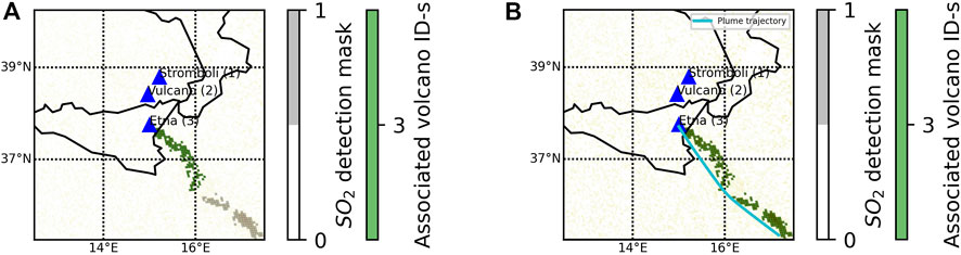
FIGURE 8. Difference in binary DBSCAN classifications (Etna volcano, on 17.06.2021). (A) Without wind. (B) With wind.
The multi-class DBSCAN algorithm (MC-1) achieves the best overall metrics, with the highest F1-score and a better accuracy. The main reference points of this algorithm are the volcano center points, making this algorithm vulnerable to areas where the spatial density of volcanoes is high, but performing well in general cases. The multi-class nature eliminates false associations that are caused by the binary classification, as shown on Figure 9C: no matter which volcano we are starting from, the plume is always going to be associated with one volcano. This is more robust than the binary classifications (Figure 9A for Dukono and Figure 9B for Ibu), where depending on the selected source volcano the plume is being associated with the currently selected one. Basically the multi-class algorithm answers the question “Which volcano does this plume originate from?”, while the binary algorithms are based on the question “Is this plume coming from the selected source volcano?”.
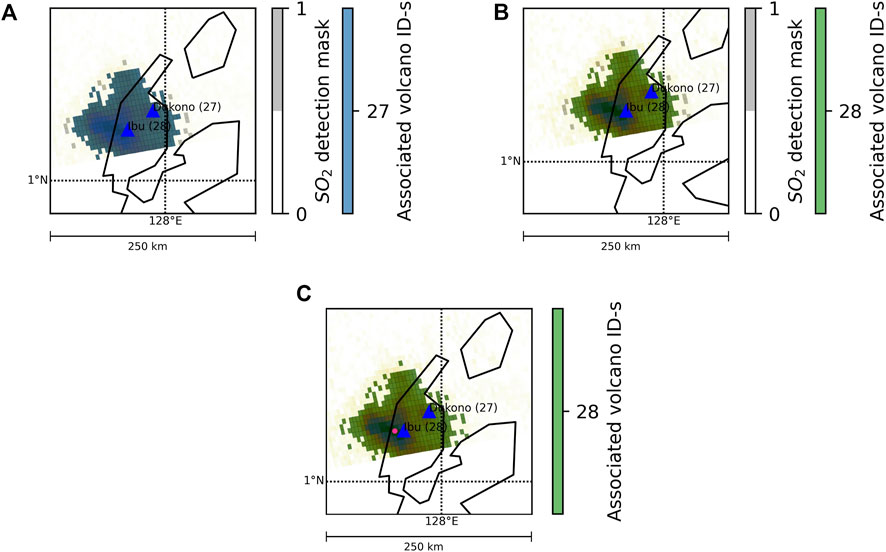
FIGURE 9. Difference in binary floodfill (A,B) vs. multi-class DBSCAN (C) classifications in an ambiguous case (Ibu volcano, on 19.03.2021). (A) Binary flood-fill with Dukono (27) as source volcano. (B) Binary flood-fill with Ibu (28) as source volcano. (C) Multi DBSCAN with Dukono (27) as source volcano.
The wind-based multi-class algorithm (MC-2) performs generally well in dense areas where plumes can travel over other volcanoes, as shown on Figure 10. However it is prone to errors in the wind models and the trajectories, which are started from the height of the nearest volcano, instead of using the actual SO2 plume height. Utilizing the multi-class approach, the plume is always associated with the volcano that is nearest to the trajectory starting from it, avoiding overlapping classifications, as shown on Figure 11B, where the small pixel cluster originating from the volcano Sheveluch is classified correctly with the multi-class method, while the binary approach fails (Figure 11A). The method generally reaches good metric values, with the F1-score being the second best in comparison, as the precision and recall values are similarly high. These results demonstrate that the multi-class method is capable of segmenting remote sensing volcanic SO2 products to multiple sources, based on both their physical features and external meteorological information.
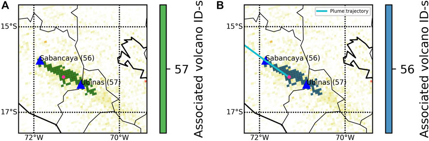
FIGURE 10. Difference in multi-class classifications in an ambiguous case (Plume from Sabancaya traveling over Ubinas volcano, on 27.04.2021). (A) Without wind data. (B) With the predicted trajectory.
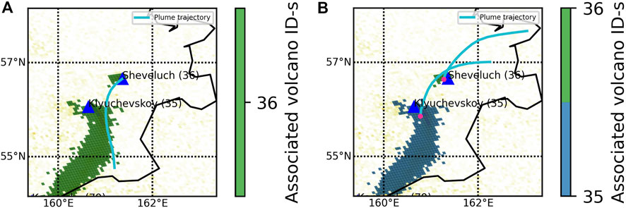
FIGURE 11. Difference in binary vs. multi-class DBSCAN classifications in an ambiguous case (Sheveluch volcano, on 19.03.2021). (A) Binary (DBSCAN with wind, with forward wind trajectory). (B) Multi-class (Multi Reverse Trajectory DBSCAN, with reverse wind trajectory).
Overall, the results follow intuitive expectations. Contrary to expectations however, the multi-class classification without wind performed slightly better than the one which uses reverse trajectories. One possible cause for this are the limitations of the meteorological models used. GDAS has a 1-degree resolution, compared to GFS, which has 0.25. Using GFS models might improve trajectory prediction, but with more data, the file size of the meteorological models increases dramatically, reducing the portability of the wind-based algorithms by a substantial amount (NCEP, NWS, NOAA, U.S. DOC, 2009). For computational reasons, only one trajectory is started from each cluster, dividing the clusters and starting multiple trajectories has the potential of improving the results, but it also greatly increases computation time. The environmental characteristics of tested volcanoes also play a role in the overall outcome. As an example, the algorithms tend to perform better with volcanoes where the plumes are generally less fragmented due to stable, continuous degassing and less wind influence. Furthermore, because the plume height is not retrieved from the TROPOMI product but rather assumed to be equal to the volcano summit altitude, the generated trajectories can suffer errors, as the strength and direction of the wind changes with the elevation.
The presented algorithms are relatively small and require limited computing time, ranging from a few milliseconds to a few seconds, with the wind-based algorithms having longer computing times as the ones without wind data. As such, they could be suited for near real-time operational volcano monitoring tasks. As the multi-class classification algorithms provides the best effectiveness/implementation complexity ratio, they are recommended for implementation in operational frameworks. Future work will focus on testing the algorithms on a larger number and variety of eruptive plumes, with the aim to implement them in monitoring systems such as MOUNTS (Valade et al., 2019).
Considering the previously presented strengths and weaknesses, the algorithms still provide room for further research and development. A first aspect to improve in the multi-class classification algorithms is the way pixel clusters are assigned to volcanoes. As of now, the assignment is based on the distance between a cluster’s center of mass (in grid space), and the volcano summit coordinates. Although this is efficient in a large majority of cases (i.e., small gas plumes, and/or plumes where the highest gas concentration is located nearby the volcano summit), it can fail in the case of strong eruption plumes, where high gas concentrations can extend several tens-hundreds of kilometers away form the emitting volcano. Indeed, this can result in the plume center of mass being off-centered with respect to the volcano, which can potentially result in erroneous associations of the SO2 plume to another non-emitting volcano closer to the plume center. An alternative to the center of mass could be using the cluster skeleton (Zhang and Suen, 1984), or the cluster shape to determine the source emission point.
Secondly, the results can be possibly improved for strong eruption plumes by incorporating near-real-time SO2 layer height retrieval, which would make the reverse trajectory calculation more deterministic and exact. As mentioned before, because the plume height is not retrieved from the TROPOMI product but rather assumed to be equal to the volcano summit altitude, the generated trajectories can suffer errors. This could be improved in the future via the SO2 Layer Height product (Hedelt et al., 2019), which provides accurate information about the height of the plumes, making reverse trajectory based algorithms more accurate (Theys et al., 2022). There are promising developments underway for that, as for major eruptions the TROPOMI SO2 Layer Height product is available. Because these products are a separate entity distinct from the actual SO2 product, and because they are only available for major eruptions, the algorithms have to query for their presence to make sure that the layer height can be retrieved. It should be stressed that using layer heights would be very useful for explosive eruption plumes having high gas concentrations and high altitudes; however they are likely to be much less useful for passive degassing plumes having have lower gas content and altitudes, as the layer height retrieval is more complicated in these cases.
As the TROPOMI L2 SO2 product is being continuously developed, the initial segmentation of volcanic SO2 detection mask is improved as well, which results in easier cluster generation, less outliers, and less false associations. This enables the lowering of ɛ values without losing outliers, although the increased number of clusters makes the trajectory generation slower and more complicated.
In the compared methods each pixel is associated with exactly one source. A future version should make a weighted attribution to multiple sources per pixel for cases of merging plumes.
In this work, we have managed to classify volcanic SO2 plume pixels in satellite imagery using classic clustering, segmentation and image processing techniques. The developed algorithms can be applied to SO2 L2 products from the Sentinel-5P TROPOMI instrument, to help with the accurate source estimation of SO2 plumes originating from various volcanoes. Furthermore, besides contributing to improving analysis and monitoring of volcanic processes from space, these algorithms can be useful in other general plume localization tasks. In particular, another potential application of the presented methods is to identify anthropogenic plume sources.
The TROPOMI SO2 data used in this paper can be downloaded from the Copernicus Open Access Hub. The Global Data Assimilation System (GDAS) meteorological files used in the trajectory generation are publicly available through the NOAA ARL FTP server. HYSPLIT is available on NOAA’s website.
BM performed the bulk of the data analysis, design and implementation of the algorithms, created the figures and wrote the first draft of the manuscript. BM, SV, and MW conceptualized the study. SV collected and analyzed the volcanic gas data. MW and OH ensured the fundamental theoretical correctness of the methods. All authors provided comments and input on the results and final version of the manuscript. Work was done as part of a BM’s Master’s Thesis, supervised by SV and MW.
We acknowledge support by the German Research Foundation and the Open Access Publication Fund of TU Berlin. SV was supported by DGAPA-PAPIIT grant IA102221.
We wish to thank the special editor Christoph Kern, as well as the two anonymous reviewers for their valuable suggestions which helped improve the manuscript. We also acknowledge the European Space Agency for providing open-access TROPOMI data, and the NOAA for providing access to GDAS meteorological models. Lastly, we wish to thank Pascal Hedelt for providing access to SO2 Layer Height products.
The authors declare that the research was conducted in the absence of any commercial or financial relationships that could be construed as a potential conflict of interest.
All claims expressed in this article are solely those of the authors and do not necessarily represent those of their affiliated organizations, or those of the publisher, the editors and the reviewers. Any product that may be evaluated in this article, or claim that may be made by its manufacturer, is not guaranteed or endorsed by the publisher.
Bernard, A., and Rose, W. I. (1990). The injection of sulfuric acid aerosols in the stratosphere by the El Chichón volcano and its related hazards to the international air traffic. Nat. Hazards (Dordr). 3, 59–67. doi:10.1007/bf00144974
Campion, R., Delgado-Granados, H., Legrand, D., Taquet, N., Boulesteix, T., Pedraza-Espitía, S., et al. (2018). Breathing and coughing: The extraordinarily high degassing of Popocatépetl volcano investigated with an SO2 camera. Front. Earth Sci. (Lausanne). 6, 163. doi:10.3389/feart.2018.00163
Carlsen, H. K., Valdimarsdóttir, U., Briem, H., Dominici, F., Finnbjornsdottir, R. G., Jóhannsson, T., et al. (2021). Severe volcanic SO2 exposure and respiratory morbidity in the Icelandic population – A register study. Environ. Health 20, 23. doi:10.1186/s12940-021-00698-y
Carn, S. A., Fioletov, V. E., McLinden, C. A., Li, C., and Krotkov, N. A. (2017). A decade of global volcanic SO2 emissions measured from space. Sci. Rep. 7, 44095. doi:10.1038/srep44095
Cofano, A., Cigna, F., Amato, L. S., de Cumis, M. S., and Tapete, D. (2021). Exploiting sentinel-5P TROPOMI and ground sensor data for the detection of volcanic SO2 plumes and activity in 2018–2021 at stromboli, 21. Basel, Switzerland: Italy. Sensors. doi:10.3390/s21216991
Corradini, S., Guerrieri, L., Brenot, H., Clarisse, L., Merucci, L., Pardini, F., et al. (2021). Tropospheric volcanic SO2 mass and flux retrievals from satellite. The Etna december 2018 eruption. Remote Sens. (Basel). 13, 2225. doi:10.3390/rs13112225
Edmonds, M., Oppenheimer, C., Pyle, D., Herd, R., and Thompson, G. (2003). So2 emissions from soufrière hills volcano and their relationship to conduit permeability, hydrothermal interaction and degassing regime. J. Volcanol. Geotherm. Res. 124, 23–43. doi:10.1016/S0377-0273(03)00041-6
Ester, M., Kriegel, H.-P., Sander, J., and Xu, X. (1996). A density-based algorithm for discovering clusters in large spatial databases with noise. KDD, 226.
Finch, D. P., Palmer, P. I., and Zhang, T. (2022). Automated detection of atmospheric NO2 plumes from satellite data: A tool to help infer anthropogenic combustion emissions. Atmos. Meas. Tech. 15, 721–733. doi:10.5194/amt-15-721-2022
Heaviside, C., Witham, C., and Vardoulakis, S. (2021). Potential health impacts from sulphur dioxide and sulphate exposure in the UK resulting from an Icelandic effusive volcanic eruption. Sci. Total Environ. 774, 145549. doi:10.1016/j.scitotenv.2021.145549
Hedelt, P., Efremenko, D. S., Loyola, D. G., Spurr, R. J. D., and Clarisse, L. (2019). Sulfur dioxide layer height retrieval from Sentinel-5 Precursor/TROPOMI using FP_ILM. Atmos. Meas. Tech. 12, 5503–5517. doi:10.5194/amt-12-5503-2019
Markus, B. (2022a). bazsimarkus/tropomi-emission-source: Initial release. Zenodo. doi:10.5281/zenodo.7311026
Markus, B. (2022b). bazsimarkus/tropomi-emission-source: Supplementary data. Zenodo. doi:10.5281/zenodo.7311105
Matthews, S. J., Gardeweg, M. C., and Sparks, R. S. J. (1997). The 1984 to 1996 cyclic activity of lascar volcano, northern Chile: Cycles of dome growth, dome subsidence, degassing and explosive eruptions. Bull. Volcanol. 59, 72–82. doi:10.1007/s004450050176
NCEP, NWS, NOAA, U.S. DOC (2009). NCEP GDAS satellite data 2004-continuing. Research Data Archive at the National Center for Atmospheric Research, Computational and Information Systems Laboratory. doi:10.5065/DWYZ-Q852
Oppenheimer, C., Fischer, T., and Scaillet, B. (2014). “Volcanic degassing: Process and impact,” in Treatise on geochemistry (Elsevier), 111–179. doi:10.1016/b978-0-08-095975-7.00304-1
Pardini, F., Corradini, S., Costa, A., Esposti Ongaro, T., Merucci, L., Neri, A., et al. (2020). Ensemble-based data assimilation of volcanic ash clouds from satellite observations: Application to the 24 december 2018 Mt. Etna explosive eruption. Atmosphere 11, 359. doi:10.3390/atmos11040359
Prata, A. J. (2009). Satellite detection of hazardous volcanic clouds and the risk to global air traffic. Nat. Hazards (Dordr). 51, 303–324. doi:10.1007/S11069-008-9273-Z
Queißer, M., Burton, M. R., Theys, N., Pardini, F., Salerno, G., Caltabiano, T., et al. (2019). TROPOMI enables high resolution SO2 flux observations from Mt. Etna, Italy, and beyond. Sci. Rep. 9, 957. doi:10.1038/s41598-018-37807-w
Robock, A. (2000). Volcanic eruptions and climate. Rev. Geophys. 38, 191–219. doi:10.1029/1998RG000054
Romahn, F., Pedergnana, M., Loyola, D., Apituley, A., Sneep, M., and Veefkind, J. P. (2022). S5P/TROPOMI L2 product user manual sulphur dioxide SO2 - S5P-L2-DLR-PUM-400E. European Space Agency.
Schmidt, A., Witham, C. S., Theys, N., Richards, N. A. D., Thordarson, T., Szpek, K., et al. (2014). Assessing hazards to aviation from sulfur dioxide emitted by explosive Icelandic eruptions. J. Geophys. Res. Atmos. 119 (14), 14, 180196–180214, 196. doi:10.1002/2014JD022070
Sierra-Vargas, M. P., Vargas-Domínguez, C., KarenBobadilla-Lozoya, C., and Aztatzi-Aguilar, O. G. (2018). Health impact of volcanic emissions. Volcanoes - Geological and geophysical setting, theoretical Aspects and numerical modeling, Applications to Industry and their Impact on the human health. Rijeka: IntechOpen. doi:10.5772/INTECHOPEN.73283
Stein, A. F., Draxler, R. R., Rolph, G., Stunder, B., Cohen, M. D., and Ngan, F. (2015). NOAA’s HYSPLIT atmospheric transport and dispersion modeling system. Bull. Am. Meteorol. Soc. 96, 2059–2077. doi:10.1175/BAMS-D-14-00110.1
Theys, N., Hedelt, P., de Smedt, I., Lerot, C., Yu, H., Vlietinck, J., et al. (2019). Global monitoring of volcanic SO2 degassing with unprecedented resolution from TROPOMI onboard Sentinel-5 Precursor. Sci. Rep. 9, 2643. doi:10.1038/s41598-019-39279-y
Theys, N., Lerot, C., Brenot, H., van Gent, J., de Smedt, I., Clarisse, L., et al. (2022). Improved retrieval of SO2 plume height from TROPOMI using an iterative Covariance-Based Retrieval Algorithm. Atmos. Meas. Tech. 15, 4801–4817. doi:10.5194/amt-15-4801-2022
Theys, N., Smedt, I. D., Yu, H., Danckaert, T., van Gent, J., Hörmann, C., et al. (2017). Sulfur dioxide retrievals from TROPOMI onboard sentinel-5 precursor: Algorithm theoretical basis. Atmos. Meas. Tech. 10, 119–153. doi:10.5194/AMT-10-119-2017
Valade, S., Ley, A., Massimetti, F., D’Hondt, O., Laiolo, M., Coppola, D., et al. (2019). Towards global volcano monitoring using multisensor Sentinel missions and artificial intelligence: The MOUNTS monitoring system. Remote Sens. (Basel). 11, 1528. doi:10.3390/RS11131528
Vincenty, T. (1975). Direct and inverse solutions of geodesics on the ellipsoid with application of nested equations. Surv. Rev. 23, 88–93. doi:10.1179/SRE.1975.23.176.88
Warner, M. S. C. (2018). Introduction to PySPLIT: A Python toolkit for NOAA ARL’s HYSPLIT model. Comput. Sci. Eng. 20, 47–62. doi:10.1109/MCSE.2017.3301549
Keywords: clustering, satellite remote sensing, semantic segmentation, SO2 volcanic plumes, volcano monitoring
Citation: Markus B, Valade S, Wöllhaf M and Hellwich O (2023) Automatic retrieval of volcanic SO2 emission source from TROPOMI products. Front. Earth Sci. 10:1064171. doi: 10.3389/feart.2022.1064171
Received: 07 October 2022; Accepted: 29 November 2022;
Published: 05 January 2023.
Edited by:
Christoph Kern, Unite○d States Geological Survey (USGS), United StatesReviewed by:
Taryn Lopez, University of Alaska Fairbanks, United StatesCopyright © 2023 Markus, Valade, Wöllhaf and Hellwich. This is an open-access article distributed under the terms of the Creative Commons Attribution License (CC BY). The use, distribution or reproduction in other forums is permitted, provided the original author(s) and the copyright owner(s) are credited and that the original publication in this journal is cited, in accordance with accepted academic practice. No use, distribution or reproduction is permitted which does not comply with these terms.
*Correspondence: Manuel Wöllhaf, d29lbGxoYWZAdHUtYmVybGluLmRl
Disclaimer: All claims expressed in this article are solely those of the authors and do not necessarily represent those of their affiliated organizations, or those of the publisher, the editors and the reviewers. Any product that may be evaluated in this article or claim that may be made by its manufacturer is not guaranteed or endorsed by the publisher.
Research integrity at Frontiers
Learn more about the work of our research integrity team to safeguard the quality of each article we publish.