 Jingru Yan
 Yushan Zhang
- China Earthquake Disaster Prevention Center, Beijing, China
In the numerical simulation of site seismic responses, traditional equivalent linearization methods typically realized in the frequency domain cannot satisfactorily analyze the high-degree non-linearity of soil under strong input motions. Therefore, the “true” non-linear numerical methods performed in the time domain are often utilized in such cases. However, a crucial element of the time-domain non-linear method, which is the hysteresis model of soil that describes the rule controlling the loading–unloading behavior of soil, has no established guidelines for earthquake engineering. Different researchers presented different models, revealing the epistemic uncertainty related to the dynamic properties of soil. Thus, the time-domain non-linear method should consider this uncertainty in practice. Therefore, in this study, a one-dimensional (1D) time-domain non-linear site seismic response analysis program was developed. The developed program was coded using Fortran95 and integrates two kinds of soil hysteresis models (i.e., extended Masing model and dynamic skeleton curve model). In both models, the damping correction was introduced to calibrate the hysteresis loop area toward the damping ratio measured in the dynamic triaxial test or resonant column test. Moreover, the temporospatial finite difference algorithm was used to resolve the 1D non-linear wave equation, and its precision was demonstrated in comparison with the results of the frequency-domain program for the linear case. Finally, the non-linear seismic response of a specific site was calculated by the proposed program. The findings of the fitting were compared to those of the two popular time-domain non-linear programs DEEPSOIL (Hashash, V6.1) and CHARSOIL (Streeter et al., CHARSOIL, Characteristics Method Applied to Soils, 1974 March 25). Simultaneously, the Japanese KIK-net strong motion observation station data were applied to validate the reliability of this program.
1 Introduction
Many data on earthquake investigation and observation show that (Seal, 1988; Gao et al., 1996; Beresnev, 2002; Kokusho et al., 2008; Kim et al., 2013) local site conditions will directly affect the ground motion amplitude, spectral characteristics, and the distribution of earthquake disaster degree. The amplification effect of ground-to-ground motion must be considered in seismic zoning, seismic safety evaluation, and seismic design analysis of engineering sites. When the ground motion parameters of engineering site design are determined, it has to consider the influence of site conditions on ground motion amplification by using corresponding adjustment methods (Li, 2013). The adjustment relationship of site ground vibration parameter should be established based on many obtained strong vibration observation data and numerical calculation results of site model. In addition, the statistical relationship of site characteristic data and ground motion property spectrum has to be analysis to determine the adjustment model of site ground vibration parameters. This requires collecting sufficient basic data for research in addition to ensuring reasonable and reliable results. Site model with numerical calculation by means of the study of field adjustment should involve the soil seismic response calculation, the construction of the theoretical model, and the reasonable descriptions on the non-linear change of stress and strain of soil constitutive relationship. In this case, it can support the large-scale site numerical model for computing platform and improve the field response calculation efficiency.
At present, the frequency-domain equivalent linearization method and time-domain non-linear (TNL) method are the most widely applied in soil seismic response analysis. The influence of site soil conditions is analyzed by using a frequency-independent equivalent linearization method in China (Bo, 1998; Li et al., 2005; Li, 2010), which is widely used in engineering due to simple concept and small calculation. However, the equivalent linearization method is often no longer applicable in weak sites with large strain and strong non-linearity (Qi et al., 2010). To ensure the calculated results being consistent with the observed results, the TNL stepwise integration rule is proposed, which is a seismic response analysis method with clear physical significance and can more truly reflect the non-linear physical process of soil under stress state (Li, 1992). The true non-linear analysis method can describe the dynamic stress-strain non-linear hysteresis model of soil (Luan et al., 1994).
There are three aspects for the one-dimensional (1D) time-domain calculation method of the site non-linear seismic response, including the model of the soil skeleton curve, the soil loading-unloading-reloading criterion, and the time-domain integration method. The soil loading-unloading-reloading criterion was firstly established by Masing in 1926 (Masing, 1926). Later, it is revised continually and the empirical function form of the skeleton curve is proposed, which is a constitutive model that can better fit the test results (Pyke, 1979; Matasovic et al., 1993; Wang et al., 1981; Li, 1992; Luan, 1992; Chen, 2006; Qi et al., 2010; Martin et al., 1982; Yee et al., 2013). At present, the TNL constitutive models are widely applied in China, including Wang Zhiliang’s extended Masing criterion (Wang et al., 1981), Li Xiaojun’s dynamic skeleton curve (Li, 1992), Luan Maotian’s true non-linear model (Luan et al., 1992), and Qi Wenhao’s UE model (Qi et al., 2010). With the development of computer technology and engineering fluctuation, various site seismic reaction analysis programs have been developed based on soil constitutive model and time-domain numerical integration methods, which are widely applied in the international geotechnical seismic engineering. At present, the internationally well-known CHARSOIL program proposed by Streeter in 1974 (Streeter et al., 1974) is based on the finite difference method and uses the Ramberg-Osgood constitutive model to reflect the dynamic non-linear characteristics of soil. It is the first TNL soil seismic response analysis program in the world. However, it uses rigid boundary conditions, so sometimes the calculation results are not consistent with the actual situation. DEEPSOIL (Hashash, 2009) is a non-linear seismic response analysis program of 1D soil layer widely used abroad. It adopts a variety of numerical analysis methods (frequency-domain equivalent linearization methods and TNL methods), and introduces several constitutive models to describe the non-linear changes of soil in the TNL method. It can be applied for different soil layer earthquake responses. In addition to that, similar programs include DesRA-2C (Idriss et al., 1968), MASH (Martin et al., 1978), D-MOD (Kavazanjian and Matasovic, 1995), and ONDA (Diego et al., 2006).
The current dilemma of the TNL methods is analyzed as follows. On the one hand, the key elements of the current TNL method, namely the soil constitutive model describing the behavior of soil addition and unloading hysteresis, is not a universally accepted rule in seismic engineering. Therefore, most research focuses on developing a more scientific and reasonable method which can actually describe the non-linear dynamic changes of soil constitutive relationship. Based on previous studies and combination of the experiment data, a simplified constitutive model for complex mathematical correction with a variety of test soil parameters can be more reasonable to describe the dynamic skeleton curve model of the relationship. However, it ignores the analysis of cognitive uncertainty related to soil dynamic properties revealed by different constitutive models. In practical engineering applications, the TNL method considers this uncertainty and the good combination of developing constitutive models and engineering applications. On the other hand, more mature international geotechnical TNL method generally exist interface interaction with poor intuition and efficiency and more complex modelling process. In addition, it gives an upper limit on the calculation scale of site model and seismic input. The research trend of the field adjustment model based on many statistical results is to adopt a variety of computational methods and constitutive models for large-scale site seismic response, so as to eliminate the uncertain impact caused by the single frequency-domain equivalent linearization method and the small calculation site type. Therefore, it is imperative to develop efficient and diversified geotechnical non-linear calculation methods with independent property rights.
This work develops a new non-linear seismic response analysis program based on Fortran95, which integrates two hysteresis models of soil, namely extended Masing criterion and dynamic skeleton curve. Meanwhile, it introduces the damping correction coefficient to calibrate the lag ring area to match the damping ratio measured in dynamic triaxial test or resonance column test. It can store data by using dynamic array technology. In principle, there is no limit on the number of site models and the calculation scale of time and space points of input and output data. The results of this work can be used for calculation of large-scale site seismic response and uncertainty analysis of site calculation method, based on which the influence characteristics of site conditions on ground motion can be studied.
2 Soil skeleton curve model
The hyperbolic skeleton model is adopted to describe the soil skeleton curve, namely, a function of strain-stress. The soil skeleton curve model is described below by taking the shear deformation as an example. The vertices of stress-strain hysteresis cycles corresponding to different strain amplitudes are connected to each other to form the soil skeleton curve, as shown in Figure 1. If any point on the skeleton curve is connected to the origin, the slope of the resulting line is the cut modulus G corresponding to the point. In addition, due to the non-linear nature of the soil, the modulus is a function of the strain, namely
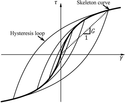
FIGURE 1. Soil skeleton curve.
If a hyperbolic function is employed to describe a 1D soil constitutive model, Eq. 1 above can be expressed as follows:
In the equation above,
In Eq. 2,
Thus:
Typically, dynamic triaxial or resonant column tests can provide discrete data between the shear modulus ratio
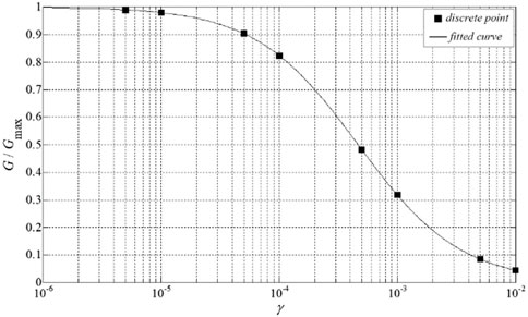
FIGURE 2. The shear modulus ratio curve.
In this work, the hyperbolic model can describe the soil skeleton curve.
3 Soil loading and unloading criterion
After the soil skeleton curve is defined, the corresponding loading and unloading criteria should be set to fully describe the loading-unloading-reloading dynamic process of the soil under the complex cyclic load. This work provides two addition and unloading criteria by previous study: extended Masing criteria proposed by Wang Zhiliang (Wang et al., 1981) and dynamic skeleton curve proposed by Li Xiaojun (Li, 1992).
3.1 Extended Masing criterion
The extended Masing criterion is widely used in seismic engineering. It is developed on the basis of Masing Criterion (Masing, 1926) and proposed by Wang Zhiliang. Its basic rules are as follows:
1) During the initial loading, the stress-strain relationship follows the skeleton curve
2) During the unloading and reverse loading, the tangent modulus at the initial unloading is equal to the maximum shear modulus
If the hyperbolic model shown in Eq. 2 is used, Eq. 6 can be expressed as follows:
In the above equations,
3) If the stress-strain curve of unloading and reverse loading intersects the skeleton curve, the subsequent stress-strain relation curve follows the skeleton curve, satisfying the “upper skeleton curve” rule;
4) If the unloaded and reverse loaded stress-strain curve intersects the previous load-unloading curve, the subsequent stress-strain curve follows the previous stress-strain curve, which is the upper circle rule.
According to the above extended Masing criterion, the 1D non-linear dynamic stress-strain relation of soil can be given for any dynamic loading process.
Figure 3 shows the hysteretic process of soil loading, unloading, and reloading under the extended Masing criterion. During the initial loading, the stress-strain relationship follows the skeleton curve, namely the 0→2 curve. If unloading is performed at point 2 and loading is realized in the direction after unloading to zero stress point 2′, the unloading-reverse loading curve follows curve 2→2′→1 in Figure 3. The unloading-reverse loading curve intersects the skeleton curve at point 1, which is symmetric about the origin. When the stress-strain relationship reaches point 1 along the curve 2→2′→1, the subsequent reverse loading curve follows the skeleton curve 1→1′. If the stress-strain relationship is reverse unloaded and reloaded along the curve 2→2′→1, the stress-strain curve follows the line 1→2. The expression of the curve 2→2′→1 can be determined by Eq. 7 according to the above rule (2). In the equation,

FIGURE 3. The extended Masing criterion (without considering damping correction).
In the above unloading-reverse loading process 2→2′→1, if reverse loading is carried out at point 3, the reverse unloading-reverse loading curve still can be determined according to Eq. 7. It illustrates that the curve determined in such way necessarily intersects the skeleton curve at point 2 and the unload-reverse loading curve 2→2′→1. Therefore, this reverse unloading-reloading curve will follow the 3→4→2 curve. If this reverse unloading-reloading process reaches point 2, then the skeleton curve is followed if loading continues, and the above unloading-reloading curve 2→2′→1 is followed if unloading.
If the reverse unloading and reloading process 3→4→2 is unloaded and reverse loaded after reaching point 4, the unloading and reverse loading curve 4→5 can be obtained by substituting the stress and strain corresponding to point 4 into Eq. 7. In this case, the extension line of the curve should meet the corresponding “big circle,” that is, the unloading and reverse loading curve 2→2′→1 of the upper layer reaches point 3. If the unloading and reverse loading process 4→5→3 reaches point 3, the subsequent reverse loading curve follows the curve 3→1 with the principle of “upper big circle” if the revserse loading continues. If this unload-reverse loading process 4→5→3 reaches point 3, the reverse unloading and reverse loading process 3→4→2 above is repeated.
The figures above illustrate the rules that should be followed in the stress-strain relationship of soil under the extended Masing criterion.
The soil-like non-linear dynamic parameter test demonstrates the relationship between shear modulus ratio and damping ratio-shear strain. An analytical representation of the soil skeleton curve can be obtained based on the relationship between the shear modulus ratio and shear strain shown in Figure 3. In combination with the above expansion Masing criteria, the soil retardation curve under equal amplitude cyclic load is obtained, including the hysteresis loops 2→2′→3→1→2 and 4→5→3→4. The area of the resulting lag loop is different from that of the damping ratio corresponding to the maximum strain (i.e., half of the difference between the maximum strain and the arrested loop). To correct this deviation, the damping correction coefficient
After that, the stress-strain relationship of soil is obtained based on the extended Masing criterion, which can be expressed as Eq. 8:
If the stress-strain state point is under the skeleton curve, the above equation is applicable for calculation; otherwise, the following equations are applicable:
In the above equations,
Equation 12 defines the correction coefficient, which is introduced for better consideration of the damping fit. The soil stress-strain change corresponding to Figure 3 is given in Figure 4, which considers the damping correction according to the hysteresis curve. It suggests that after the damping correction, the “double” relationship between the unloading-reverse loading curve and the skeleton curve is no longer satisfied, and the area of the damping correction is the same as the damping circle corresponding to the test damping ratio. Moreover, for the correction case shown in the figure, the two branches of the hysteresis curve intersect in the skeleton curve. In this case, the unloading-reverse loading curve determined in Eq. 8 intersects the skeleton curve in advance without adopting the “upper skeleton curve” criterion. In Figure 4, the unloading-reverse loading curve 2→2′→3→1 intersects the skeleton curve even at the point 3′, but the upper skeleton curve criterion is followed at point 1. Therefore, both the “upper skeleton curve” criterion and the “upper large circle” criterion are based on whether the current stress-strain curve reaches and exceeds the previous inflection point. For the first loading, the first inflection point appears (point 2 in Figure 4), then the previous inflection point is symmetrical with the origin (point 1). Therefore, the unloading-reverse loading process from point 2 follows the curve 2→2′→3→1.
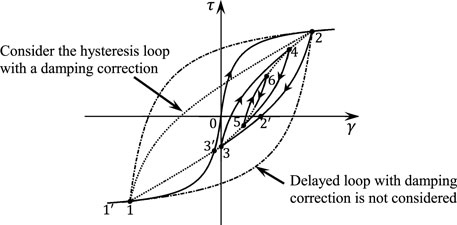
FIGURE 4. Extended Masing criterion (damping correction not considered).
3.2 Dynamic skeleton curve criteria
When the soil stress-strain arrest behavior is described by using the extended Masing criteria, it should repeatedly remember and identify the current inflection point and its previous inflection point. It will be more complex and detrimental to programs when the cyclic load is complex (such as ground motion input). Due to the complexity and uncertainty of the dynamic characteristics of the soil, the hysteresis criterion based on the dynamic skeleton curve proposed by Li (1992) remembers and identifies the current inflection point and the maximum inflection point of stress-strain history while showing the basic characteristics of the Masing criterion, so it is easier to implement.
The dynamic skeleton curve describes the loading-unloading hysteresis criterion for 1D soil based on the following three basic hypotheses:
1) During the initial loading, the stress-strain relationship curve coincides with the soil skeleton curve;
2) During the unloading and reverse loading, the stress-strain relationship curve directly points to the absolute maximum stress-strain point of the stress-strain history or its reverse symmetry point, enabling that the stress and strain relationship curve and the skeleton curve meet the “double” relationship for the equal amplitude cyclic load process;
3) The stress and strain relationship curve of the subsequent loading process after meeting with the skeleton curve will follow the skeleton curve.
The above hypotheses are not the exactly same as those of the extended Masing criterion, where it assumes that hypothesis (3) is the “upper skeleton curve” criterion. The biggest difference between the two is the above hypothesis (2). In the extended Masing criterion, the unloading-reverse loading stress-strain relationship curve points to the previous inflection point of the current inflection point. While in the dynamic skeleton curve criterion, it points directly to the absolute maximum stress-strain point of the stress-strain history or its reverse symmetry point.
According to the above hypotheses, the relationship between soil shear stress and strain corresponding to the hyperbolic dynamic skeleton curve criterion can be obtained as follows:
In the above relationship,
Equation 17 is the same form as Eq. 12, but the definition
Without the damping correction,
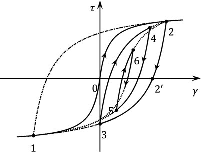
FIGURE 5. Dynamic skeleton curve criterion (damping correction not considered).
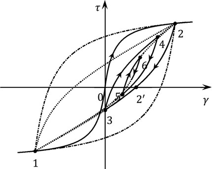
FIGURE 6. Dynamic skeleton curve criterion (damping correction considered).
3.3 Time-space finite difference method
In this work, the finite difference method is employed to discretize the time-domain and the space-domain. The dynamic equilibrium equation of the 1D wave can be written as follows:
The deformation coordination condition is expressed as follows:
The non-linear constitutive equation between stress and strain is expressed as follows:
In the several equations above,
Before the dynamic equation difference is solved differentially, each soil layer should be subdivided according to corresponding stability conditions of the differential format. Because the space-time center difference scheme is adopted to solve the dynamic equation in this work, the thickness of each soil layer after the subdivision layer should satisfy Eq. 21 below:
To ensure smaller calculation error caused by spatial discretization, the thickness of each calculated soil should satisfy the below relationship as much as possible:
After spatial-temporal discretization of Eqs 18–20 by using the central difference method, the following explicit difference stepwise integral scheme can be acquired:
They can be rewritten as follows:
In the equations above.
The Eq. 24 is adopted to combine the boundary conditions with initial conditions, it can gradually integrate the velocity of the medium at the top of each layer and the shear stress and shear strain response of the medium at the midpoint of the layer. The corresponding acceleration and displacement can be derived from the velocity response quantity. The initial conditions for calculation are as follows:
The boundary conditions are defined as follows:
In Eq. 28,
In the above equation,
Figure 7 presents the explicit space-time finite difference grids. Among them, solid points indicate the known initial conditions or boundary conditions, hollow points represent the spacetime points to be solved, square points mark the stress (or strain) spacetime points, and circular points represent the velocity spacetime points. According to the grid, the speed and stress at each space-time point can be gradually found.

FIGURE 7. Space-time explicit finite difference grid.
In the above time-domain numerical integration method, the discretized time interval ∆t should be small enough to ensure computational stability due to the application of central difference algorithm. Thickness of soil calculation stratification should meet the requirements of Eq. 21.
4 Numerical examples
This section employs several basic numerical examples to validate the reliability of the time-domain non-linear calculation program developed for this paper.
4.1 Example 1
This example verifies the accuracy of the time-space finite difference method, which is introduced in the field seismic response by comparing with an ideal two-layer field and a complex multi-layer field of an actual major project.
As for the mechanical parameters of the two models (Tables 1, 2), site 1 is an ideal two-storey site, and site 2 is a complex multi-storey site for a practical major project, which contains a hard interlayer with thickness of 15.9 m. In this example, all media are assumed to be linear elastic media, and the damping ratio is set to 0.05. Meanwhile, site-2 was chosen to verify the accuracy of the time-space finite difference method when the difference between the upper and lower soil layers is significant. Whereupon, a comparison is performed between the numerical solution and the analytical solution.
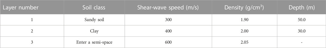
TABLE 1. Computational model of site 1.
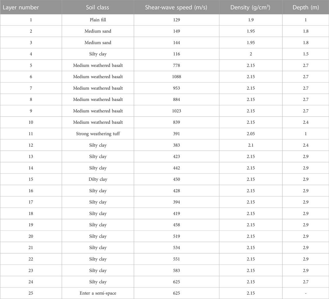
TABLE 2. Computational model of site 2.
The time history curves of upgoing waves at the top of input half space in terms of accelerated speed, velocity and displacement (incident wave) are indicated in Figure 8. Under the ground motion input as indicated in Figure 8, the time-history curve of ground motion on site 1 surface obtained with the time-space finite difference method as described in Section 3.3 is compared with the calculation result obtained with the frequency domain method, as shown in Figure 9, with the comparison result of response spectrum curve presented in Figure 10. Figures 11, 12 indicate the corresponding results of site 2.
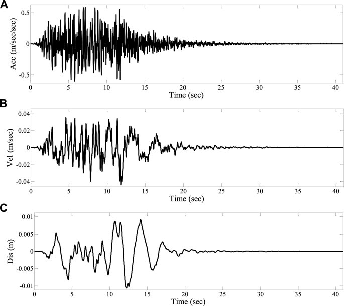
FIGURE 8. Time history curve of upgoing wave at the top of input half space (A) Accelerated speed. (B) Velocity. (C) Displacement.
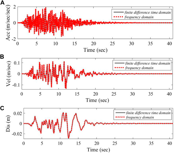
FIGURE 9. Comparison between ground motion time history curves of site 1. (A) Accelerated speed. (B) Velocity. (C) Displacement.
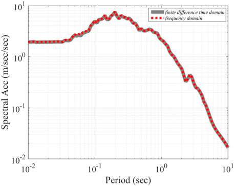
FIGURE 10. Comparison of ground motion response spectrum curves of site 1.
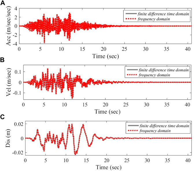
FIGURE 11. Comparison between ground motion time history curves of site 2. (A) Accelerated speed. (B) Velocity. (C) Displacement.
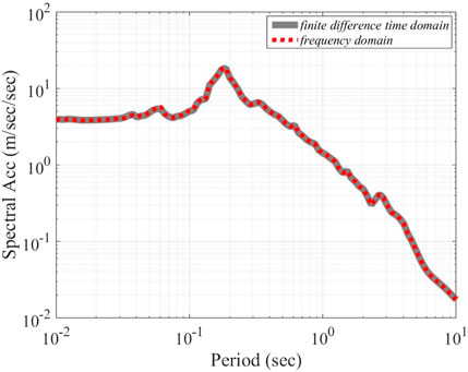
FIGURE 12. Comparison of ground motion response spectrum curves of site 2.
It can be observed that the calculation results of the two methods are basically consistent. It needs to be noted that the time-space finite difference method adopts the central difference method to replace the time and spatial derivatives of the wave equation, and then it determines the numerical solution of the fluctuation problem by explicit numerical integration, while the frequency domain method determines the analytical expression of the steady-state solution followed by the transient reaction by Fourier transformation. Moreover, when referring to the time-space finite difference method, the artificial boundary processing method is adopted to handle the infinite domain problem of the input half space, while the frequency domain method may eliminate the infinite domain truncation problem, without considering the exact accuracy of the numerical error of the discrete Fourier transformation itself. The consistency of the calculation results as presented in Figures 9–12 indicates that it is reliable to solve one-dimensional site seismic response with time-space finite difference method by the numerical program developed in this work.
4.2 Example 2
In this section, the data from a certain practical engineering site and the KiK-net station was introduced. With contrastive analysis of DEEPSOIL (Hashash, V6.1) and CHARSOIL (Streeter et al., 1974), the non-linear time-domain programs used worldwide, the reliability of the program developed herein was further demonstrated.
Presently, DEEPSOIL is the most extensively adopted time-domain non-linear soil layer seismic response analysis and calculation program in the world, representing the highest level of time-domain non-linear analysis. Therefore, in this section, the actual project site with silt soil layer is used as the calculation model (the mechanical parameters of the model are shown in Table 3). The Northridge strong seismic observation data is used as input for a comparative analysis of the proposed method (the constitutive model adopts the extended Masing criterion, same as below) and the DEEPSOIL time domain algorithm. Figures 13, 14 depict the calculated surface acceleration time history and response spectrum. In comparison, the proposed method is consistent with the time-history curve of surface acceleration calculated by DEEPSOIL, with a marginally lower amplitude than the DEEPSOIL results. According to the comparison curves of the reaction spectrum, the proposed method for fitting the long-period reaction spectrum is relatively consistent. While the high-frequency component is less than the DEEPSOIL calculation results. The reason for the difference is inferred to be the difference between the backbone curves of the non-linear constitutive model of rock and soil and the finite difference method utilized by the two programs.
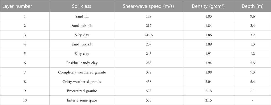
TABLE 3. Computational model of site 3.
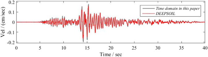
FIGURE 13. Comparison between ground motion time history curves of site 3 (Accelerated speed).
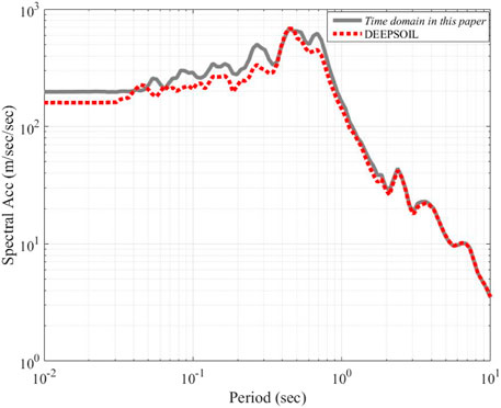
FIGURE 14. Comparison of ground motion response spectrum curves of site 3.
Observation station data from the Japanese KiK-net network at a class II site are used concomitantly. The observation point is used as the input; and by comparing and analyzing the calculation results of various time-domain non-linear programs (the proposed method, DEEPSOIL, CHARSOIL) with the actual surface observation records corresponding to the observation points, the reliability of the non-linear program in this paper is verified.
Figure 15 depicts the comparison results of the seismic response spectrum curve at the surface. In accordance with the figure, the research methodology and DEEPSOIL calculation findings are comparable to the actual surface observation record. The overall reaction spectrum curve is essentially consistent with the actual surface observation record, especially the curves of the long period (T > 2 s), which completely overlap, with the exception of the large fitting error of individual reaction spectrum periods (such as T = 0.5 s ∼ 1 s). Whereas the GHARSOIL calculation result represents a significant error.
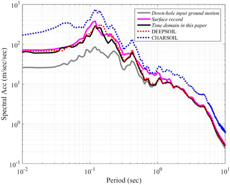
FIGURE 15. Comparison of ground motion response spectrum curves of different programs with actual observation records.
In terms of this section, the non-linear method is comparable to the internationally recognized DEEPSOIL program’s calculation results and is superior to the CHARSOIL when compared to actual observation records. In contrast to DEEPSOIL, the developed procedure is simple, quick, and has a high modeling efficiency, particularly when the site soil layer is thick and the soil is abundant.
5 Conclusion
In order to solve the problems such as the uncertainty of site non-linear seismic response results caused by a single calculation method and the restriction of traditional site non-linear calculation program on the calculation scale, a site non-linear seismic response analysis program is developed based on fortran95 software platform for the time-space finite difference method in this work. To facilitate the consideration of the uncertainty effect of various soil constitutive models under the TNL method, the program is embedded in two relatively mature soil constitutive models at the present stage, namely the extended Masing criterion model and the dynamic skeleton curve model. Simultaneously, port is reserved for the further introduction of various soil constitutive models, and it can be a tool platform for the uncertainty research work of soil non-linear dynamic change. Moreover, the program uses dynamic array technology to store relevant data, and it has no limitation on the computational scale of the site model, the time points and space points of the input and output data principally. In addition, the program can be used for large-scale site seismic response calculation work, and facilitate the research work of site adjustment coefficient in the new generation of zoning map in China. Finally, the reliability of the developed calculation program are verified based on the practical examples, and through a comparative analysis of a relatively mature time-domain non-linear program and testing with actual records from the KiK-net strong motion observation station in Japan, the time-nonlinear program developed in this paper demonstrates a high degree of calculation reliability and modeling efficiency. Consequently, it is applicable to the calculation of more complex site conditions and large-scale site seismic response. Due to the singularity and uniqueness of the example model, additional real site models should be included in the follow-up work to validate the procedure’s applicability. Moreover, an uncertainty analysis of various site calculation methods should be carried out.
Data availability statement
The raw data supporting the conclusion of this article will be made available by the authors, without undue reservation.
Author contributions
All authors listed have made a contribution to conception and design of the study, and approved it for publication. Main program development: YZ. Collection and processing of data: YZ and JY. Writing-original draft: JY. Writing-reviewing and editing: YZ and JY. All authors contributed to manuscript revision, read, and approved the submitted version.
Funding
This study is supported by the Science for Earthquake Resilience of China Earthquake Administration (XH22013YA).
Conflict of interest
The authors declare that the research was conducted in the absence of any commercial or financial relationships that could be construed as a potential conflict of interest.
Publisher’s note
All claims expressed in this article are solely those of the authors and do not necessarily represent those of their affiliated organizations, or those of the publisher, the editors and the reviewers. Any product that may be evaluated in this article, or claim that may be made by its manufacturer, is not guaranteed or endorsed by the publisher.
References
Beresnev, I. A. (2002). Nonlinearity at California generic soil sites from modeling recent strong-motion data. Bull. Seismol. Soc. Am. 92 (2), 863–870. doi:10.1785/0120000263
Bo, J. S. (1998). Site Classification and design response spectrum adjustment method (postdoctoral research Report). China Earthquake Administration: Institute of Engineering Mechanics, 55–58.
Chen, X. L. (2006). Study on soil dynamic properties, and nonlinear seismic response of complex site and its methods. China Earthquake Administration, Institute of Engineering Mechanics.
Diego, C. F. L. P., Carlo, G. L., and Ignazio, P. (2006). ONDA: Computer code for nonlinear seismic response analyses of soil deposits. J. Geotech. Geoenviron. Eng. 132 (2), 223–236.
Gao, S., Liu, H., and Davis, P. M., (1996). Localized amplification of seismic waves and correlation with damage due to the northridge earthquake: Evidence for focusing in santa monica. Bull. Seismol. Soc. Am. 869 (1B), 209–230.
Idriss, I. M., and Seed, H. B. (1968). Seismic response of horizontal soil layers. Soil Mechanics and Foundations Division. J. Soil Mech. Found. Div. 94 (4), 1003–1031. doi:10.1061/jsfeaq.0001163
Kavazanjian, E., and Matasovic, N. (1995)., 46. New Orleans, Louisiana, USA, 1066–1080.Seismic analysis of solid waste landfillsGeoenvironmental 2000, Geotech. Spec. Publ.2
Kim, B., and Hashash, Y. M. A. (2013). Site response analysis using downhole array recordings during the march 2011 tohoku-oki earthquake and the effect of long-duration ground motions. Earthq. Spectra 29 (S1), 37–54. doi:10.1193/1.4000114
Kokusho, T., and Sato, K. (2008). Surface-to-base amplification evaluated from KiK-net vertical array strong motion records. Soil Dyn. Earthq. Eng. 28 (9), 707–716. doi:10.1016/j.soildyn.2007.10.016
Li, P. (2010). The effect of site types on platform value of the design response spectrum. China Earthquake Administration: Harbin: Institute of Engineering Mechanics.
Li, X. J. (1992). A method for analysing seismic response of nonlinear soil layers. South China J. Seismol. 12 (4), 1–8.
Li, X. J. (1992). A simple function expression of the soil dynamic constitutive relationship. Chin. J. Geotechnical Eng. (05), 90–94.
Li, X. J. (2013). Adjustment of seismic ground motion parameters considering site effects in seismic zonation map. Chin. J. Geotechnical Eng. 35 (S2), 21–29.
Li, Y. Y., Xu, Y., and Li, D. M. (2005). Analysis of earthquake responses for different site categories. Earthq. Res. Shanxi 4, 27–33.
Luan, M. T., and Lin, G. (1994). An effective time-domain computational method for nonlinear seismic response analysis of soil deposit. J. Dalian Univ. Technol. 34 (2), 228–234.
Luan, M. T., and Lin, G. (1992). Computational model for nonlinear analysis of soil site seismic response. Eng. Mech. 9 (1), 94–103.
Luan, M. T. (1992). Ramberg-osgood constitutive model with variable parameters for dynamic nonlinear analysis of soils. Earthq. Eng. Eng. Vib. (02), 69–78.
Martin, P. P., and Seed, H. B. (1982). One-dimensional dynamic ground response analyses. J. Geotech. Engrg. Div. 108 (7), 935–952. doi:10.1061/ajgeb6.0001316
Martin, P. P., and Seed, H. B. (1978). MASH-A computer program for the non-linear analysis of vertically propagating shear waves in horizontally layered deposits. Calif: Report EERC, University of California at Berkeley, 78–23.
Masing, G. (1926). Eigenspannungeu and verfertigung beim Messing. Zurich: Proceedings of the 2nd International Congress on Applied Mechanics.
Matasovic, N., and Vucetic, M. (1993). Cyclic characterization of liquefiable sands. J. Geotech. Engrg. 119 (11), 1805–1822. doi:10.1061/(asce)0733-9410(1993)119:11(1805)
Pyke, R. M. (1979). Nonlinear soil models for irregular cyclic loadings. J. Geotech. Engrg. Div. 105 (6), 715–726. doi:10.1061/ajgeb6.0000820
Qi, W. H., Wang, Z. Q., and Bo, J. S. (2010). Development and verification of a method for analyzing the nonlinear seismic response of soil layers. J. Harbin Eng. Univ. 31 (4), 444–450.
Qi, W. H., and WangBo, Z. Q, J. S. (2010). Development and verification of a method for analyzing the nonlinear seismic response of soil layers. J. Harbin Eng. Univ. 31 (04), 444–450.
Seed, H. B., Romo, M. P., Sun, J. I., Jaime, A., and Lysmer, J. (1988). The Mexico earthquake of september 19, 1985: Relationships between soil conditions and earthquake ground motions. Earthq. Spectra 4 (4), 687–729. doi:10.1193/1.1585498
Streeter, V. L., Wylie, E. B., and Richart, F. E. (1974). CHARSOIL, 100(3), 247-263, characteristics method applied to soils.
Wang, Z. L., and Han, Q. Y. (1981). Analysis of wave propagation for the site seismic response, using the visco-elastoplastic model. Earthq. Eng. Eng. Vibraion (01), 117–137.
Keywords: soil dynamics, soil modulus, non-linear hysteretic response, backbone curve, soil seismic response
Citation: Yan J and Zhang Y (2023) One dimensional time-domain non-linear site seismic response analysis program integrating two hysteresis models of soil. Front. Earth Sci. 10:1058386. doi: 10.3389/feart.2022.1058386
Received: 30 September 2022; Accepted: 05 December 2022;
Published: 30 January 2023.
Edited by:
Yefei Ren, China Earthquake Administration, ChinaReviewed by:
Ba Zhenning, Tianjin University, ChinaYushi Wang, Beijing University of Technology, China
Copyright © 2023 Yan and Zhang. This is an open-access article distributed under the terms of the Creative Commons Attribution License (CC BY). The use, distribution or reproduction in other forums is permitted, provided the original author(s) and the copyright owner(s) are credited and that the original publication in this journal is cited, in accordance with accepted academic practice. No use, distribution or reproduction is permitted which does not comply with these terms.
*Correspondence: Yushan Zhang, aHlzemhhbmdAMTYzLmNvbQ==