 Hongyun Jiao
 Junju Xie
 Mi Zhao2
 Juke Wang
95% of researchers rate our articles as excellent or good
Learn more about the work of our research integrity team to safeguard the quality of each article we publish.
Find out more
ORIGINAL RESEARCH article
Front. Earth Sci. , 04 January 2023
Sec. Structural Geology and Tectonics
Volume 10 - 2022 | https://doi.org/10.3389/feart.2022.1057316
This article is part of the Research Topic Measuring, Modeling and Predicting the Seismic Site Effect View all 20 articles
This study proposes a seismic input method for layered slope sites exposed to obliquely-incident seismic waves which transforms the waves into equivalent nodal forces that act on the truncated boundary of a finite element model. The equivalent nodal forces at the left and right boundaries are obtained by combining the free field response of a one-dimensional layered model with a viscoelastic boundary. The equivalent nodal forces at the bottom boundary are obtained by combining the incident wave field with the viscoelastic boundary. This proposed seismic input method for slope sites exposed to obliquely incident seismic waves is implemented with the aid of MATLAB software; it is applied to the seismic response analysis of slope sites in the commercial finite element ABAQUS software. The calculation results are compared with the reference solutions obtained by using the extended model to verify the correctness of the established seismic input method. The proposed seismic input method is then employed to investigate the influencing factors of the seismic response of layered slope sites exposed to oblique incidence P waves. The results show that the angle of incidence, location of the interface between soft and hard rocks, and impedance ratio have significant effects on the seismic landslide.
Landslides are frequent during earthquakes in mountainous and hilly areas (Prestininzi and Romeo, 2000; Chigira et al., 2005; Sato et al., 2007; Semblat et al., 2011). Hillside topography can magnify seismic intensity and change seismic frequency content—termed “topographic effects”. Landslide disasters caused by earthquakes have been a frequent subject of geological hazard research because of their wide distribution, considerable quantity, and great harm (Bird et al., 2004; Owen et al., 2008). Since the 1960s, scholars have begun identifying and analyzing the seismic response of slope sites exposed to seismic waves (Cavallin and Slejko, 1986; Jibson et al., 2000; Pareek and Arora, 2010; Li et al., 2022). Analysis methods have included landslide observation, model testing, and numerical simulations (Keeper, 1984). The finite element method (FEM) is the most common numerical method; it can effectively simulate the geometric and material non-linear characteristics of slope sites.
When analyzing the seismic response of slope sites based on FEM, it is necessary to introduce artificial boundary conditions at the truncated boundaries of the finite domain to simulate the radiation damping effect of the infinite domain on the finite domain. The artificial boundary appropriate to the characteristics and specific conditions of the research object must be deduced. Due to the irregular terrain of slope sites, poor geological conditions, and the existence of free surfaces, the topographic effect of slope site has attracted research attention (Gischig et al., 2015; Poursartip et al., 2017). It is necessary to deduce the appropriate artificial boundary according to the characteristics of the research object and the specific situation. In previous finite element analysis of the seismic response of slope sites, most scholars have assumed that the bottom boundary of the model is rigid, while the lateral side boundaries adopt roller boundaries (Rizzitano et al., 2014), viscous boundaries (Lysmer and Kuhlemeyer, 1969; Athanasopoulo et al., 1999; Pelekis, 2017), viscoelastic boundaries (Deeks and Randolph, 1994; Liu et al., 2006; Maleki and Khodakarami, 2017), transmissive boundaries (Liao and Wong, 1984), paraxial approximate boundaries (Clayton and Engquist, 1977), and infinite element boundaries (Bettess, 1977; Astley, 2000). Seismic input is completed by converting the seismic wave action into the equivalent forces applied to boundaries; however, this treatment method is not applicable in cases where the lower part of the site model is not bedrock.
Much recent research has been conducted on the seismic response analysis of slope sites with non-rigid bedrock at the bottom of the site model. Based on the viscous boundary, Bouckovalas and Papadimitriou (2005) presented numerical analyses for the seismic response of step-like ground slopes in uniform viscoelastic soil under vertically propagating SV seismic waves. Assimaki et al. (2005) employed the viscous boundary to address vertically incident seismic wave action and obtained a seismic input method suitable for layered slopes. Based on the viscous boundary, Lenti and Martino (2012) studied a landslide disaster on a stepped slope under the action of a vertically incident seismic wave. Nakamura (2012) adopted the energy-transmitting boundary to study the seismic input and established the seismic response analysis method for the layered slope. However, when the source is shallow or the site is far from the epicenter, the seismic input cannot be assumed to be vertically incident seismic waves but can be considered obliquely incident.
Scholars have thus conducted research on the seismic response of regular sites under the action of obliquely incident seismic waves. Liu and Lu (1998) proposed a seismic input method based on spring-buffer boundary conditions that convert seismic waves with arbitrary incident angles into equivalent nodal forces acting on boundary nodes. Based on the viscoelasticity boundary, Huang et al. (2017a) and Huang et al. (2017b) used the FEM to analyze the non-linear seismic response of tunnels with a normal fault ground subjected to obliquely incident seismic waves. Bazyar and Song (2017) expressed such a wave as the boundary condition applied to the near field by the proportional boundary FEM. Based on the one-dimensional time-domain FEM proposed by Liu and Wang (2007), Zhao et al. (2013) and Zhao et al. (2017) proposed an improvement by establishing a site response analysis method and applying it to study the influence of the oblique incidence of ground motion on the seismic response of subway stations. However, previous seismic input methods have been established for seismic response analysis of regular sites under the action of obliquely incident seismic waves; this is not applicable to the seismic response of slope sites under the action of obliquely incident seismic waves. There are few studies on the seismic input method of slope sites exposed to obliquely incident seismic waves.
In this paper, obliquely incident seismic waves are transformed into equivalent nodal forces that act on the truncated boundary of the finite element model as the seismic input. Based on the viscoelastic artificial boundary, the free field responses of one-dimensional layered sites with different heights are taken as the seismic input for the left and right boundaries, and the incident wave field is used as the seismic input for the bottom. Then, the proposed seismic input method for slope sites under the action of obliquely incident seismic waves is implemented with the aid of MATLAB software and is applied to the seismic response analysis of slope sites in the commercial finite element ABAQUS software. Accordingly, the numerical simulation results of a two-dimensional layered slope site obtained using the established seismic input method are compared with the numerical results of an extended computational model to verify the accuracy of this method. Finally, with the aid of the proposed seismic input method, the influencing factors of the seismic response of layered slope sites under oblique incidence P waves are determined.
Figure 1A illustrates the schematic diagram of the seismic response analysis of a layered slope site subjected to P waves obliquely incident at an angle of α. When analyzing the seismic response of a two-dimensional layered slope site with the aid of the FEM, the finite computational domain needs to be cut off from the infinite ground. Artificial boundaries are usually used to simulate waves scattered by target structures and the non-reflecting wave effect of truncated infinite domains (Du et al., 2006; Huang et al., 2016; Zhao et al., 2019; Li et al., 2020). The stable and accurate viscoelasticity artificial boundary developed by Du et al. (2006) is adopted in this study. For a given boundary node l (xl, yl, zl), one pair of dashpots and springs in the normal and tangential directions of the boundary plane are established respectively (Figure 1B).
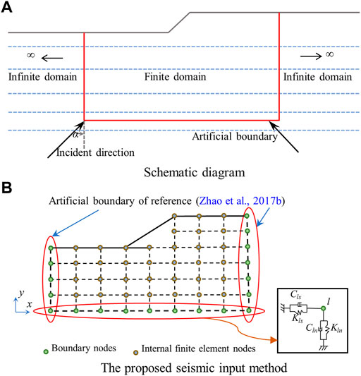
FIGURE 1. Model of a layered slope site under obliquely incident P waves. (A) Schematic diagram. (B) Proposed seismic input method.
At a given boundary node l (xl, yl) of the 2-D finite element model, the parameters for the springs and dashpots are
where Kln and Kls denote the normal and tangential spring stiffnesses at the boundary node l (xl, yl); Cln and Cls denote the normal and tangential damping coefficients at the boundary node l (xl, yl); Al is half of the total length of all boundary elements containing the boundary node l (xl, yl); R is the distance between the scattering source and the artificial boundary node; λ, G, and ρ are the Lamé constant, shear modulus, and mass density of the ground, respectively; cs and cp represent the shear and compression wave velocities of the ground, respectively; ar and br are the modified coefficients with good values of 0.8 and 1.1, respectively (Du et al., 2006).
The dynamic finite element equation for the finite domain has the form
where subscript B represents the boundary node and subscript I represents the internal node,
The seismic waves can be separated into the free field motion of the infinite domain and scattering wave motion generated by all scattering sources. The free field motion in the infinite domain or engineering site is expressed by the superscript f, and the scattering wave motion is expressed by the superscript s. The displacement
where
where
Substituting Eqs 3–5 into Eq. 6 after rearrangement, the following equation can be obtained:
where
Then, substituting Eq. 7 into Eq. 2, the dynamic finite element equation is:
where submatrices [CB] and [KB] are both diagonal. For the boundary node l (xl, yl), [CB]l = Cl, [KB]l = Kl. [Ff] represents the equivalent seismic forces acting on the artificial boundary.
Equation 9 provides the method of converting seismic waves into equivalent nodal forces that act on artificial boundary nodes to realize the seismic wave input in the seismic response analysis of the finite element model. To calculate the equivalent node force at each boundary node, it is necessary to provide the free field velocity, displacement, and stress at the node.
For the incidence of the seismic waves, the wave motions can be transferred into equivalent node forces applied at the boundary nodes. However, due to the topographic effect of the slope site, the seismic input wave fields at the left, right, and bottom boundaries of the two-dimensional finite element model are different. Realization of the seismic wave input at the left and right artificial boundaries requires the free field response calculation for a one-dimensional layered site. Because of the different heights of the left and right sides of the slope terrain, one-dimensional FEM calculations are necessary (Figure 2) (Zhao et al., 2017). The equivalent nodal forces at the left and right boundaries are then obtained by combining the calculation results of the one-dimensional FEM with the viscoelastic artificial boundary to complete the seismic input at the left and right boundaries.
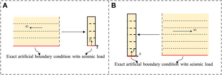
FIGURE 2. One-dimensional finite element model. (A) Left boundary. (B) Right boundary.
For node l (xl, yl) on the left or right boundary, the equivalent nodal forces of obliquely incident P waves can be given as
where
For node l (xl, 0) on the bottom boundary, the equivalent nodal forces of obliquely incident P waves can be given as
where
Since the P waves are obliquely incident at an angle of α, there is a time delay in the response of any node on the bottom boundary relative to that of the initial incident node in the finite element model.
where
The stresses along and perpendicular to the incident direction of the P wave are expressed as
The stresses
The seismic input method established in Section 2 is realized through programming with MATLAB software and is applied to the seismic response analysis of slope sites in the commercial finite element ABAQUS software. To verify the accuracy of the proposed seismic input method, this section simulates the free field response of a layered slope site under the action of obliquely incident P waves. The size of the finite element model of the two-dimensional slope site is 240 m long, 70 m high on the left side, and 100 m high on the right side (Figure 3). h represents the thickness of soft layer; in this section, h = 30 m. The reference solution is the calculation result of an extended computational model with a length of 4100 m, a right-side height of 2100 m, and a left-side height of 2070 m. The slope site is meshed by solid elements, with a mesh size of 1 m. The material parameters of each layer of the slope site are shown in Table 1 (JTG/T D70-2010, 2010). The form of the obliquely incident pulse wave with an incident angle of α acting on the slope site calculation model is shown in Figure 4.

FIGURE 3. Calculation model for the layered slope site exposed to obliquely incident P waves.
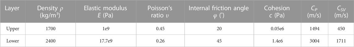
TABLE 1. Material constants of the soil.
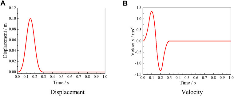
FIGURE 4. Time history curve of the input seismic wave. (A) Displacement. (B) Velocity.
In verifying the seismic input method for the layered slope site, the P wave is incident from the left corner of the model with angles of 0°, 10°, 20°, and 30°. The observation nodes are arranged at each node of the free surface within the range of 10 m from the left side of the slope toe to 10 m from the right side of the slope top (Figure 3). Top node A and toe node B are the main observation nodes. The results of the acceleration, velocity, and displacement time history of the layered slope site model, calculated on the established seismic input method, are compared with the results of the extended model. The comparison results are shown in Figure 5. The results obtained with the aid of the established seismic input method agree well with the reference solutions. The accuracy and applicability of the established seismic wave input method for slope sites are thus verified.
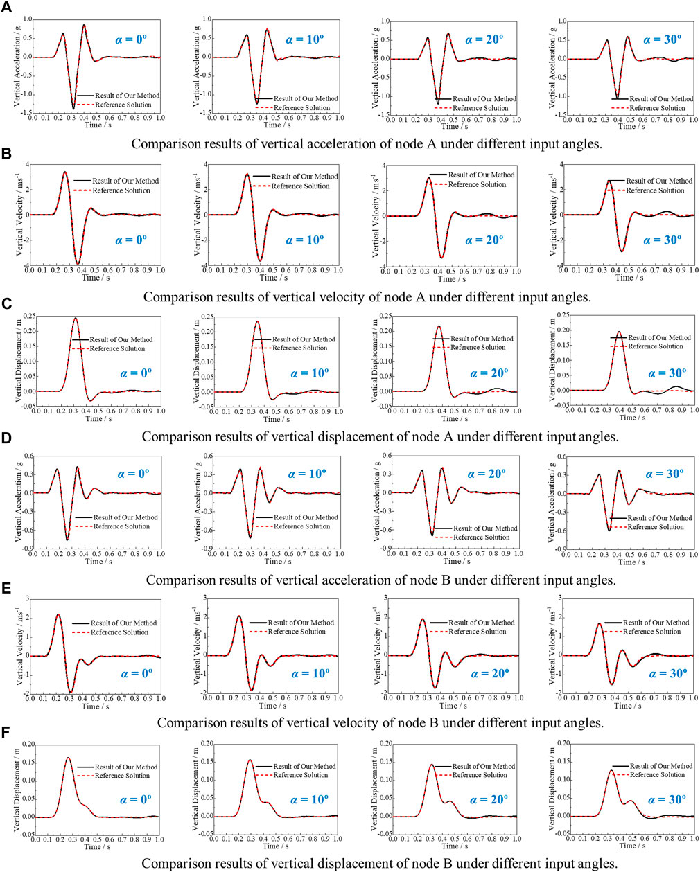
FIGURE 5. Comparison results at different input angles. (A) Comparison of the vertical acceleration results of node A at different input angles. (B) Comparison of the vertical velocity results of node A at different input angles. (C) Comparison of the vertical displacement results of node A at different input angles. (D) Comparison of the vertical acceleration results of node B at different input angles. (E) Comparison of the vertical velocity results of node B at different input angles. (F) Comparison of the vertical displacement results of node B at different input angles.
The relative error of the peak displacement value is used to measure the accuracy of the calculation results; the calculation formula is
where r0(t) is the displacement reference solution, r(t) is the displacement calculation result obtained using the seismic input method proposed in this paper, | | represents the absolute value, and the subscript max is used to evaluate the maximum value.
The comparison of the results and relative errors of the vertical displacement peaks of each observation node on the free surface are shown in Figure 6. The change in the dynamic amplification effect of the displacement peak with topographic relief is negligible, and the maximum error of the displacement peak at four incident angles is less than 1%. Therefore, by comparing the calculated results of the small model of the slope site with the numerical results of the extended model, the high accuracy of the developed seismic input method is further demonstrated.
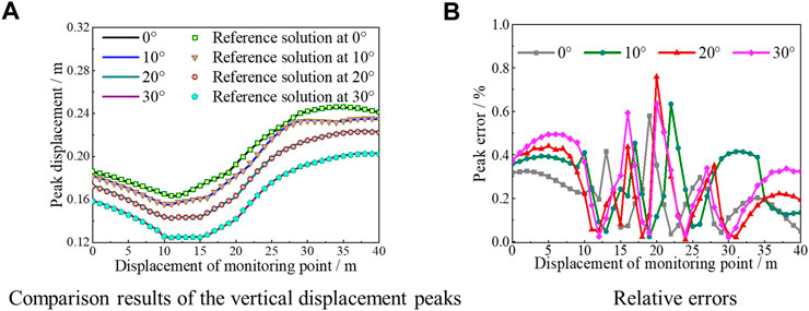
FIGURE 6. Comparison of the results and relative errors of the vertical displacement peaks of each observation node on the free surface. (A) Comparison of the results of the vertical displacement peaks. (B) Relative errors.
This section discusses the effects of incident angles, soft-hard rock interface positions, and impedance ratios on the seismic responses of slope sites exposed to obliquely incident P waves. The seismic input method of the slope site established in Section 2 is employed.
The upper soft rock and lower hard rock of the slope site is modeled in ABAQUS software, and the Mohr-Coulomb elastic-plastic model is selected for the constitutive relationship. The model dimensions are shown in Figure 3. The Kobe wave (Figure 7) is input by the seismic input method proposed in this paper to study the factors that influence seismic landslides.
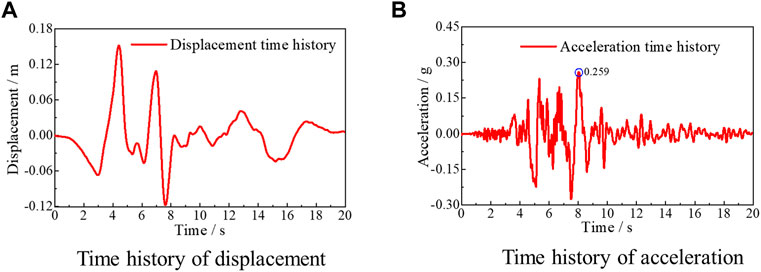
FIGURE 7. Time histories of the Kobe wave for Kobe University. (A) Time history of displacement. (B) Time history of acceleration.
This subsection investigates the influence of the different incident angles (α = 0°, 15°, 30°, and 45°) of P waves on the dynamic responses of the slope site. The site parameters are shown in Table 1, with the soft and hard rock interface 30 m from the slope top. Figure 8 shows the plastic strain nephograms of the slope site at different timing exposed to obliquely incident P waves with different angles. The displacement nephograms of the slope site at t = 20 s are illustrated in Figure 9A.
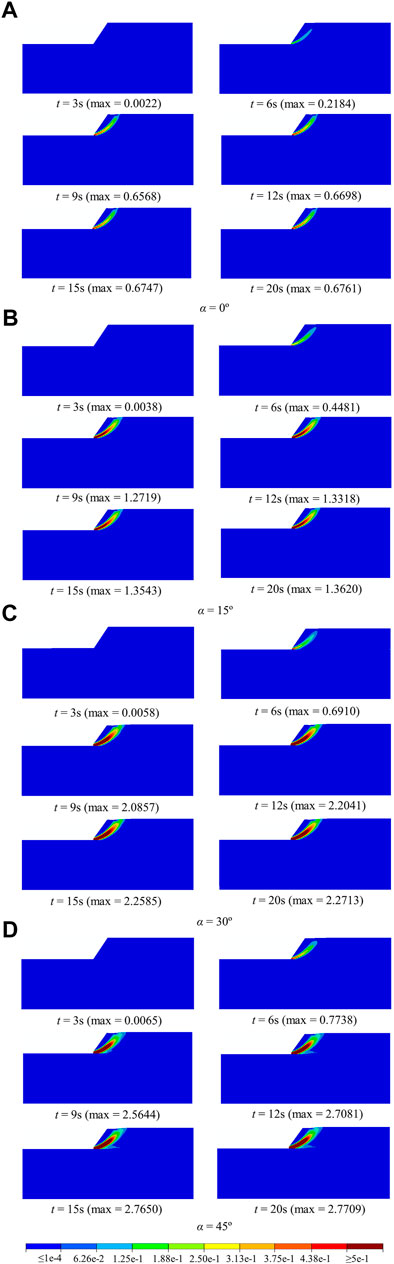
FIGURE 8. Plastic strain nephograms of the slope at different timing with different incident angles. (A) α = 0°. (B) α = 15°. (C) α = 30°. (D) α = 45°.
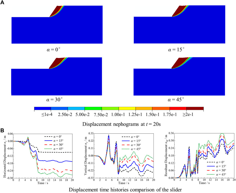
FIGURE 9. Displacement of the slope at different incident angles. (A) Displacement nephograms at t = 20 s. (B) Displacement time history comparison of the slider.
As shown in Figure 8, landslides occur in the slope sites of upper soft rock and lower hard rock exposed to obliquely incident P waves with different incident angles. Landslide surfaces appear on the slope bodies, and the blocks slide down along the landslide surfaces. With increasing incident angle, the maximum plastic strain value increases, and the plastic zone of the slope site enlarges. Meanwhile, the landslide surface starts earlier at larger incident angles. Figure 9A shows that the volume and sliding displacement of the landslide mass increase with an increasing incident angle, and the sliding slope surface changes from steep to gentle. This means that the landslide hazard becomes higher with an increase in the oblique incidence angle of the P wave.
To better reflect the displacement of each slider at different incident angles, Figure 9B shows the displacement time history comparison of a slider at such angles. As shown in Figure 9B, the absolute value of the horizontal average displacement of the slider increases with an increase of the incident angle, while the absolute value of the vertical average displacement decreases. The resultant displacement of the sliding block first decreases and then increases with an increase of the incidence angle, and the corresponding deformation of the slope site gradually changes from elastic to plastic deformation.
This subsection analyzes the effect of the soft and hard rock interface positions on the dynamic response of the slope site by adopting the slope site model of the upper soft rock and lower hard rock shown in Figure 3. The distances between the soft–hard rock interface and the slope top are h = 30, 27, 24, and 21 m, respectively. The smaller the distance between the soft-hard rock interface and the slope top, the thinner the soft rock overburden is above the hard rock. The site parameters are shown in Table 1.
P waves are obliquely incident at an angle of α = 45° from the lower left corner of the model. Figure 10 shows the plastic strain nephograms of the slope site under the action of obliquely incident P waves with different soft–hard rock interface positions at different timings. Figure 11A depicts the displacement nephograms of the slope site at t = 20 s. Figures 10, 11A show that, for the slope site with upper soft rock and lower hard rock, the plastic zones first appear at the interfaces between soft rock and hard rock and then continuously develop upward to form landslide surfaces. A thicker soft-rock overburden tends to cause an earlier appearance of the plastic strain zone, faster sliding surface formation, a greater plastic zone and plastic deformation, and stronger sliding.
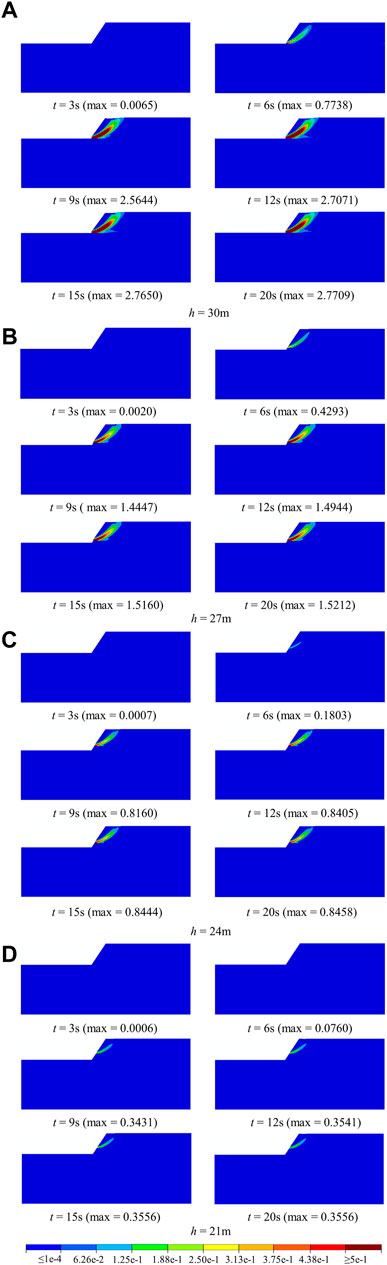
FIGURE 10. Plastic strain nephograms of the slope at different timings with different soft–hard rock interface positions. (A) h = 30 m. (B) h = 27 m. (C) h = 24 m. (D) h = 21 m.
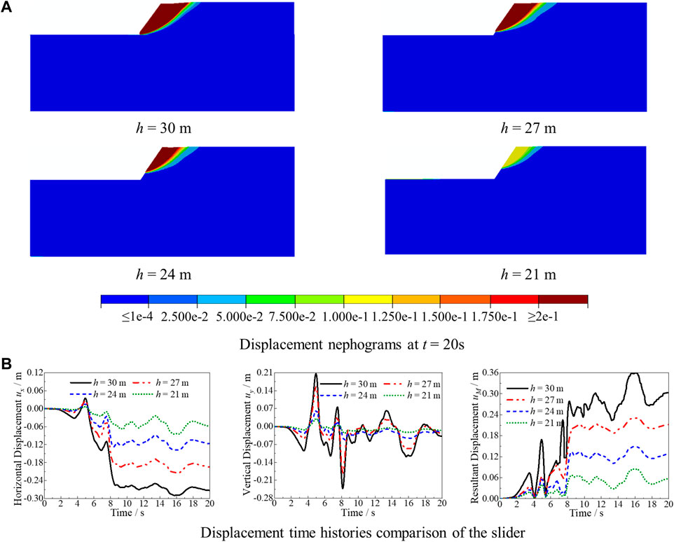
FIGURE 11. Displacement of the slope at different interface positions of soft and hard rock. (A) Displacement nephograms at t = 20 s. (B) Displacement time history comparison of the slider.
In order to better reflect the influence of the soft–hard rock interface position on the sliding displacement of the slider, Figure 11B describes the displacement time history comparison results of the slider at different positions of the soft–hard rock interface. Thus, the absolute value of the horizontal and vertical average displacement and the resultant displacement of the slider all increase as the distance between the soft–hard rock interface to the top of the slope changes from near to far.
According to the comprehensive analysis in Figures 10, 11, on slope sites of upper soft rock and lower hard rock, the smaller the thickness of the soft rock layer, the safer the site will be. When the interface between soft and hard rock is 21 m from the slope top, the plastic strain zone appears late, and the plastic strain and sliding displacement of the slider are small. The thickness of soft rock is small enough to prevent landslides.
This subsection analyzes the dynamic responses of the layered slope site at different impedance ratios (η = 0.2, 0.4, 0.6, 0.8, and 1.0) of the upper and lower layers. The size of the slope site finite element model is the same as in Section 4.1; the site parameters are shown in Table 2. P waves are obliquely incident at an angle of α = 15° from the lower left corner of the model.
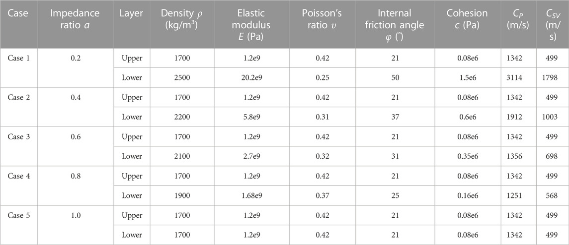
TABLE 2. Material constants of the slope site.
Plastic strain nephograms of the slope with different impedance ratios are given in Figure 12. The greater the impedance ratio between the upper and lower media, the later the plastic strain zone appears, the slower the development speed, and the later the landslide surface will occur. The maximum plastic strain of the slope site decreases with increasing impedance ratio between the upper and lower media.
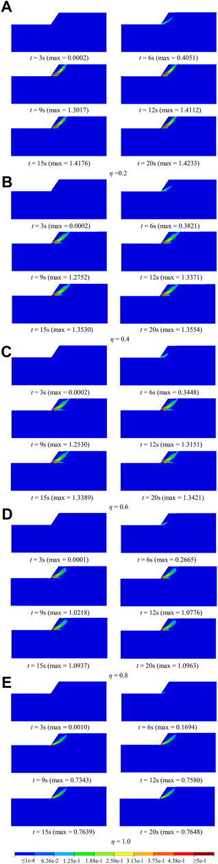
FIGURE 12. Plastic strain nephograms of the slope at different timing with different impedance ratios. (A) η = 0.2. (B) η = 0.4. (C) η = 0.6. (D) η = 0.8. (E) η = 1.0.
Figure 13A illustrates the displacement nephograms of the slope site with different impedance ratios at t = 20 s. The impedance ratio has no effect on the position of the landslide surface and the volume of the sliding block but has a significant effect on the sliding displacement of the sliding block.
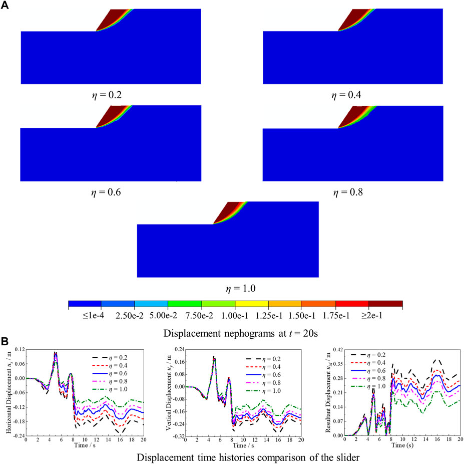
FIGURE 13. Displacement of the slope at different impedance ratios. (A) Displacement nephograms at t = 20 s. (B) Displacement time history comparison of the slider.
To better reflect the influence of the impedance ratio between the upper and lower media on the sliding displacement of the slider, Figure 13B describes the displacement time history comparison results of the slider at different impedance ratios. It can be concluded that the absolute value of the horizontal and vertical average displacement and the resultant displacement of the slider have the same change trend under different impedance ratios, and that they all decrease with the increase in impedance ratio. With this increase, the landslide hazard of the slope site decreases significantly.
Landslide seismic disasters have become a focus of geological hazard research because of their wide distribution, frequency, and great harm. Due to the topographic effect of slope sites, the seismic input method of regular sites is no longer applicable. This paper combines viscoelastic boundary with a seismic input method for slope sites under the action of obliquely incident P waves. Application is made with MATLAB programming software. The finite element model of the slope site is established in the application software ABAQUS, and the seismic mechanical behavior of the slope site is simulated by the Mohr-Coulomb model. Compared with the calculation results of the extended model, the established seismic input method is verified as correct. The established seismic input method is applied to analyze the parameters of landslide disasters in slope sites with upper soft rock and lower hard rock.
Under all calculation working conditions, the landslide hazard occurrence process of the slope site is basically the same, but the severity of the landslide hazard is different. Under the action of obliquely incident P waves, a small range of plastic deformation in upper soft rock slopes and lower hard rock slopes first occurs at the soft–hard rock interface. Next, the plastic zone expands upward to form a small-scale plastic zone, and the maximum plastic strain value increases continuously; the input velocity time history is then close to the peak. Thereafter, the plastic zone expands upward. When the input seismic wave reaches peak value, an obvious slip surface is formed. The slope body slides downward along this, and the deformation of the slope top is obvious. After the peak value is reached, there is no obvious change in the size of the plastic zone, but the maximum plastic strain value still increases in a small range over time. The details are as follows.
(1) For the slope site with upper soft rock and lower hard rock, the plastic zone and plastic strain value increase as the incident angle of the P wave changes from 0° to 45°. The larger the incident angle of the P wave, the earlier the landslide surface will form, the larger the landslide volume and sliding displacement, and the more serious the landslide disaster will be.
(2) For slope sites with upper soft rock and lower hard rock, the plastic zones first appear at the soft–hard rock interface and then continuously develop upward to form the landslide surfaces. The farther the soft–hard interface is from the slope top, the earlier the plastic strain zone will appear, and the faster the slip surface forms. With the thickening of the soft rock overburden, the plastic zone area and plastic deformation increase, and the sliding displacement of the slider is more obvious.
(3) The greater the impedance ratio between the upper and lower media of the layered slope site, the later the plastic strain zone will appear, and the slower the plastic zone develops. At different impedance ratios, the location of the landslide surface and the volume of the sliding block are basically the same. The maximum plastic strain and sliding displacement of the sliding block decrease with the increase of impedance ratio.
Some limitations should be noted with this paper. As the type of seismic failure of hard rock slopes is different from that studied in this paper, the proposed method is not suitable for such slopes. These conclusions and findings are based on the simulation results of the calculation model of the soft rock slope site and slope site with upper soft rock and lower hard rock. Due to the complexity of the problems, the validity of these conclusions and findings for calculating a model of hard rock slope sites or soil slope sites need much more study. Moreover, the simulation of the material of the slope site is based on the Mohr-Coulomb model without considering the existence of cracks and structural planes in rock mass materials. In general, the limits mentioned above should be addressed in future work.
Finally, the proposed method only discusses seismic landslides under the action of P waves, and further research is needed on seismic landslides under the action of shear waves and Rayleigh waves. Follow-up study regarding these issues is needed.
The original contributions presented in the study are included in the article/supplementary material; further inquiries can be directed to the corresponding author.
HJ: data curation, writing—original draft preparation, and program. JX: conceptualization, writing-reviewing, and fund support. MZ: guide the establishment of method and writing-reviewing. JH: software and assist in the establishment of the method. XD: resources, supervision, writing—review and editing. JW: visualization and data curation.
This work was supported by Postdoctoral Science Foundation of China (2022M722929), the Special Fund of the Institute of Geophysics, China Earthquake Administration (DQJB20B23), and Beijing Natural Science Foundation Program (JQ19029). The support is gratefully acknowledged.
The authors declare that the research was conducted in the absence of any commercial or financial relationships that could be construed as a potential conflict of interest.
All claims expressed in this article are solely those of the authors and do not necessarily represent those of their affiliated organizations, or those of the publisher, the editors and the reviewers. Any product that may be evaluated in this article, or claim that may be made by its manufacturer, is not guaranteed or endorsed by the publisher.
Assimaki, D., Gazetas, G., and Kausel, E. (2005). Effects of local soil conditions on the topographic aggravation of seismic motion: Parametric investigation and recorded field evidence from the 1999 athens earthquake. Bull. Seismol. Soc. Am. 95 (3), 1059–1089. doi:10.1785/0120040055
Astley, R. J. (2000). Infinite elements for wave problems: A review of current formulations and an assessment of accuracy. Int. J. Numer. Methods Eng. 49 (7), 951–976. doi:10.1002/1097-0207(20001110)49:7<951::aid-nme989>3.0.co;2-t
Athanasopoulos, G. A., Pelekis, P. C., and Leonidou, E. A. (1999). Effects of surface topography on seismic ground response in the Egion (Greece) 15 June 1995 earthquake. Soil Dyn. Earthq. Eng. 18 (2), 135–149. doi:10.1016/s0267-7261(98)00041-4
Bazyar, M. H., and Song, C. (2017). Analysis of transient wave scattering and its applications to site response analysis using the scaled boundary finite-element method. Soil Dyn. Earthq. Eng. 98, 191–205. doi:10.1016/j.soildyn.2017.04.010
Bettess, P. (1977). Infinite elements. Int. J. Numer. Methods Eng. 11 (1), 53–64. doi:10.1002/nme.1620110107
Bird, J. F., and Bommer, J. J. (2004). Earthquake losses due to ground failure. Eng. Geol. 75 (2), 147–179. doi:10.1016/j.enggeo.2004.05.006
Bouckovalas, G. D., and Papadimitriou, A. G. (2005). Numerical evaluation of slope topography effects on seismic ground motion. Soil Dyn. Earthq. Eng. 25 (7-10), 547–558. doi:10.1016/j.soildyn.2004.11.008
Cavallin, A., and Slejko, D. (1986). Statistical approach to landslide and soil liquefaction hazards in seismic areas. Geol. Appl. E Idrogeol. 21 (2), 231–236.
Chigira, M., and Yagi, H. (2005). Geological and geomorphological characteristics of landslides triggered by the 2004 Mid Niigta prefecture earthquake in Japan. Eng. Geol. 82 (4), 202–221. doi:10.1016/j.enggeo.2005.10.006
Clayton, R., and Engquist, B. (1977). Absorbing boundary conditions for acoustic and elastic wave equations. Bull. Seismol. Soc. Am. 67 (6), 1529–1540. doi:10.1785/bssa0670061529
Deeks, A. J., and Randolph, M. F. (1994). Axisymmetric time-domain transmitting boundaries. J. Eng. Mech. 120 (1), 25–42. doi:10.1061/(asce)0733-9399(1994)120:1(25)
Du, X. L., Zhao, M., and Wang, J. T. (2006). A stress artificial boundary in FEA for near-field wave problem. Chin. J. Theor. Appl. Mech. 38, 49–56.
Gischig, V. S., Eberhardt, E., Moore, J. R., and Hungr, O. (2015). On the seismic response of deep-seated rock slope instabilities—insights from numerical modeling. Eng. Geol. 193, 1–18. doi:10.1016/j.enggeo.2015.04.003
Huang, J. Q., Du, X. L., Jin, L., and Zhao, M. (2016). Impact of incident angles of P waves on the dynamic responses of long lined tunnels. Earthq. Eng. Struct. Dyn. 45 (15), 2435–2454. doi:10.1002/eqe.2772
Huang, J. Q., Du, X. L., Zhao, M., and Zhao, X. (2017b). Impact of incident angles of earthquake shear (S) waves on 3-D non-linear seismic responses of long lined tunnels. Eng. Geol. 222, 168–185. doi:10.1016/j.enggeo.2017.03.017
Huang, J. Q., Zhao, M., and Du, X. L. (2017a). Non-linear seismic responses of tunnels within normal fault ground under obliquely incident P waves. Tunn. Undergr. Space Technol. 61, 26–39. doi:10.1016/j.tust.2016.09.006
Jibson, R. W., Harp, E. L., and Michael, J. A. (2000). A method for producing digital probabilistic seismic landslide hazard maps. Eng. Geol. 58 (3), 271–289. doi:10.1016/s0013-7952(00)00039-9
JTG/T D70-2010 (2010). Guidelines for Design of Highway Tunnel. The People’s Republic of China: Industry Recommended Standards of the People’s Republic of China, 35–48 (In Chinese).
Keeper, D. K. (1984). Landslides caused by earthquakes. Geol. Soc. Am. Bull. 95 (4), 406. doi:10.1130/0016-7606(1984)95<406:lcbe>2.0.co;2
Lenti, L., and Martino, S. (2012). The interaction of seismic waves with step-like slopes and its influence on landslide movements. Eng. Geol. 126, 19–36. doi:10.1016/j.enggeo.2011.12.002
Li, C., He, J., Wang, Y., and Wang, G. (2022). A novel approach to probabilistic seismic landslide hazard mapping using Monte Carlo simulations. Eng. Geol. 301, 106616. doi:10.1016/j.enggeo.2022.106616
Li, H. F., Zhao, M., and Du, X. L. (2020). Accurate H-shaped absorbing boundary condition in frequency domain for scalar wave propagation in layered half-space. Int. J. Numer. Methods Eng. 121, 4268–4291. doi:10.1002/nme.6424
Liao, Z. P., and Wong, H. L. (1984). A transmitting boundary for the numerical simulation of elastic wave propagation. Int. J. Soil Dyn. Earthq. Eng. 3 (4), 174–183. doi:10.1016/0261-7277(84)90033-0
Liu, J. B., Du, Y. X., Du, X. L., Wang, Z. Y., and Wu, J. (2006). 3D viscous-spring artificial boundary in time domain. Earthq. Engin. Engin. Vib. 5 (1), 93–102. doi:10.1007/s11803-006-0585-2
Liu, J. B., and Lu, Y. D. (1998). A direct method for analysis of dynamic soil-structure interaction based on interface idea. Dev. Geotechnical Eng. 83 (3), 261–276. doi:10.1016/s0165-1250(98)80018-7
Liu, J. B., and Wang, Y. (2007). A 1D Time-domain method for inplane wave motion of free field in layered media. Chin. J. Eng. Mech. 24 (7), 16–22.
Lysmer, J., and Kuhlemeyer, R. L. (1969). Finite dynamic model for infinite media. J. Engrg. Mech. Div. 95 (4), 859–877. doi:10.1061/jmcea3.0001144
Maleki, M., and Khodakarami, M. I. (2017). Feasibility analysis of using MetaSoil scatterers on the attenuation of seismic amplification in a site with triangular hill due to SV-waves. Soil Dyn. Earthq. Eng. 100, 169–182. doi:10.1016/j.soildyn.2017.05.036
Nakamura, N. (2012). Two-dimensional energy transmitting boundary in the time domain. Earthquakes Struct. 3 (2), 97–115. doi:10.12989/eas.2012.3.2.097
Owen, L. A., Kamp, U., Khattak, G. A., Harp, E. L., Keefer, D. K., and Bauer, M. A. (2008). Landslides triggered by the 8 october 2005 kashmir earthquake. Geomorphology 94 (1-2), 1–9. doi:10.1016/j.geomorph.2007.04.007
Pareek, N., Arora, S., and Arora, M. K. (2010). Impact of seismic factors on landslide susceptibility zonation: A case study in part of Indian himalayas. Landslides 7, 191–201. doi:10.1007/s10346-009-0192-1
Pelekis, P., Batilas, A., Pefani, E., Vlachakis, V., and Athanasopoulos, G. (2017). Surface topography and site stratigraphy effects on the seismic response of a slope in the Achaia-Ilia (Greece) 2008 Mw6. 4 earthquake. Soil Dyn. Earthq. Eng. 100, 538–554. doi:10.1016/j.soildyn.2017.05.038
Poursartip, B., Fathi, A., and Kallivokas, L. F. (2017). Seismic wave amplification by topographic features: A parametric study. Soil Dyn. Earthq. Eng. 92, 503–527. doi:10.1016/j.soildyn.2016.10.031
Prestininzi, A., and Romeo, R. W. (2000). Earthquake-induced ground failures in Italy. Eng. Geol. 58 (3-4), 387–397. doi:10.1016/s0013-7952(00)00044-2
Rizzitano, S., Cascone, E., and Biondi, G. (2014). Coupling of topographic and stratigraphic effects on seismic response of slopes through 2D linear and equivalent linear analyses. Soil Dyn. Earthq. Eng. 67, 66–84. doi:10.1016/j.soildyn.2014.09.003
Sato, P. H., Hasegawa, H., Fujiwara, S., Tobita, M., Koarai, M., Une, H., et al. (2007). Interpretation of landslide distribution triggered by the 2005 Northern Pakistan earthquake using SPOT 5 imagery. Landslides 4 (2), 113–122. doi:10.1007/s10346-006-0069-5
Semblat, J. F. (2011). Modeling seismic wave propagation and amplification in 1D/2D/3D linear and nonlinear unbounded media. Int. J. Geomech. 11 (6), 440–448. doi:10.1061/(asce)gm.1943-5622.0000023
Zhao, M., Gao, Z. D., Du, X. L., Wang, J. T., and Zhong, Z. L. (2019). Response spectrum method for seismic soil-structure interaction analysis of underground structure. Bull. Earthq. Eng. 17, 5339–5363. doi:10.1007/s10518-019-00673-6
Zhao, M., Gao, Z. D., Wang, L. T., Du, X. L., Huang, J. Q., and Li, Y. (2017). Obliquely incident earthquake input for soil-structure interaction in layered half space. Earthquakes Struct. 13 (06), 573–588.
Keywords: seismic input method, obliquely incident P waves, layered slope site, influencing factors, seismic landslide
Citation: Jiao H, Xie J, Zhao M, Huang J, Du X and Wang J (2023) Seismic response analysis of slope sites exposed to obliquely incident P waves. Front. Earth Sci. 10:1057316. doi: 10.3389/feart.2022.1057316
Received: 29 September 2022; Accepted: 05 December 2022;
Published: 04 January 2023.
Edited by:
Yefei Ren, Institute of Engineering Mechanics, China Earthquake Administration, ChinaReviewed by:
Zhang Yushan, China Earthquake Disaster Prevention Centre, ChinaCopyright © 2023 Jiao, Xie, Zhao, Huang, Du and Wang. This is an open-access article distributed under the terms of the Creative Commons Attribution License (CC BY). The use, distribution or reproduction in other forums is permitted, provided the original author(s) and the copyright owner(s) are credited and that the original publication in this journal is cited, in accordance with accepted academic practice. No use, distribution or reproduction is permitted which does not comply with these terms.
*Correspondence: Junju Xie, eGllanVuanYwNUBtYWlscy51Y2FzLmFjLmNu
Disclaimer: All claims expressed in this article are solely those of the authors and do not necessarily represent those of their affiliated organizations, or those of the publisher, the editors and the reviewers. Any product that may be evaluated in this article or claim that may be made by its manufacturer is not guaranteed or endorsed by the publisher.
Research integrity at Frontiers
Learn more about the work of our research integrity team to safeguard the quality of each article we publish.