Strategy for eliminating high-frequency instability caused by multi-transmitting boundary in numerical simulation of seismic site effect

A multi-transmitting boundary is a local artificial boundary widely used for numerically simulating seismic site effects. However, similar to other artificial boundaries, the multi-transmitting boundary has instability issue in numerical simulation. Based on the concept of multi-directional transmitting formula, a strategy for eliminating the high-frequency instability of the transmitting boundary is studied and a measure is proposed using a neighbour node of a boundary node to realize smoothing filtering. The proposed measure is verified through numerical analysis. The smoothing coefficient chosen for this measure provides a reference for deriving the coefficient of multidirectional transmitting formula in the time domain.

1 Introduction

The influence of local topography on ground motion is fundamentally a wave scattering problem. Hence, simulating near-field waves is crucial to the numerical simulation of seismic site effects. The accuracy of near-field wave numerical simulations directly depends on whether artificial boundary conditions can accurately simulate an infinite domain. Since the 1960s, several achievements have been attained in the study of artificial boundaries (Liao, 1984, 2002; Wolf, 1988; Givoli, 1992; Cheng et al., 1995; Wolf, 1996; Xu et al., 2018; Xing et al., 2021). Among the established artificial boundary conditions, the multi-transmitting boundary (Liao et al., 1984a; Liao et al., 1984b; Xing et al., 2017a; Xing et al., 2017b) has a wide application range and high precision. Moreover, combined with the finite element method, the multi-transmitting boundary can facilitate decoupling.

Similar to other local artificial boundaries, the transmitting boundary’s computational stability is a key issue that requires further study. High-frequency oscillation and low-frequency drift are two types of numerical instability phenomena that may occur when the multi-transmission boundary is combined with the finite element method (Li et al., 2012; Yang et al., 2014). In this paper, a strategy for eliminating the instability of high-frequency oscillations of the multi-transmission boundary is suggested.

Smoothing factor filtering is an effective measure for restraining high-frequency instability of transmission boundary (Liao et al., 1989; Liao et al., 1992; Liao et al., 2002). Another measure to restrain high-frequency instability is utilizing the energy consumption characteristics of explicit integration scheme. This measure inhibits high-frequency instability by increasing damping in proportion to strain velocity (Li et al., 1992; Li et al., 2007; Tang et al., 2010). Modifying the internal node motion equation and stiffness of the finite element is also an effective measure for stabilizing the high-frequency of multi-transmission boundary (Xie et al., 2012; Zhang et al., 2021).

This paper proposes an improved measure for existing strategies to restrain high-frequency instability using a smoothing factor. When considering only the high-frequency error oscillation perpendicular to the artificial boundary and ignoring the high-frequency oscillation parallel to the artificial boundary, the current method only smooths the points perpendicular to the boundary. Based on the concept of a multidirectional transmitting formula, this paper proposes smoothing the points on the artificial boundary to restrain high-frequency instability.

2 Multi-transmitting formula and its instability of high-frequency oscillation for restraining instability

2.1 Multi-transmitting formula (MTF)

The multi-transmitting boundary is also called Multi-transmitting formula (MTF), which is a boundary condition using the general expression of a one-sided traveling wave solution to simulate an external wave crossing the boundary at a point on the artificial boundary. It uses internal point displacement to represent the boundary point displacement. MTF was proposed by Liao et al. (Liao, 1984, 2002). In the finite element discrete model (Figure 1), the MTF of the arbitrary artificial boundary point J can be expressed as

${\mathit{u}}_{\mathit{J}}^{\mathit{P}+\mathbf{1}}={\displaystyle \sum }_{\mathit{n}=\mathbf{1}}^{\mathit{N}}{\left(-\mathbf{1}\right)}^{\mathit{n}+\mathbf{1}}{\mathit{C}}_{\mathit{n}}^{\mathit{N}}\overline{{\mathit{T}}_{\mathit{n}}}\overline{{\mathit{u}}_{\mathit{n}}}(1)$

where J of ${\mathit{u}}_{\mathit{J}}^{\mathit{P}+\mathbf{1}}$ represents the position in the discrete grid (e.g., point J in Figure 1), P + 1 of ${\mathit{u}}_{\mathit{J}}^{\mathit{P}+1}$ represents moment P+1, N is the order of MTF, and ${\mathit{C}}_{\mathit{n}}^{\mathit{N}}$ is a binomial coefficient (${\mathit{C}}_{\mathit{n}}^{\mathit{N}}=\mathit{N}!/\left(\left(\mathit{N}-\mathit{n}\right)!\mathit{n}!\right)$). The following yields $\overline{{\mathit{T}}_{\mathit{n}}}$ and $\overline{{\mathit{u}}_{\mathit{n}}}$:

$\left\{\begin{array}{l}\overline{{\mathit{u}}_{\mathit{n}}}={\left[{\mathit{u}}_{\mathit{J}}^{\mathit{P}-\mathit{n}+\mathbf{1}},{\mathit{u}}_{\mathit{J}-\mathbf{1}}^{\mathit{P}-\mathit{n}+\mathbf{1}},\cdots ,{\mathit{u}}_{\mathit{J}-\mathbf{2}\mathit{n}}^{\mathit{P}-\mathit{n}+\mathbf{1}}\right]}^{\mathit{T}}\\ \overline{{\mathit{T}}_{\mathit{n}}}=\left[{\mathit{T}}_{\mathbf{1}},{\mathit{T}}_{\mathbf{2}},\cdots ,{\mathit{T}}_{\mathbf{2}\mathit{n}+\mathbf{1}}\right]\\ {\mathit{T}}_{\mathit{K}}=\sum {\mathit{t}}_{{\mathit{K}}_{\mathbf{1}}}{\mathit{t}}_{{\mathit{K}}_{\mathbf{2}}}\cdots {\mathit{t}}_{{\mathit{K}}_{\mathit{n}}}\left(K=\mathbf{1,2},\cdots ,\mathbf{2}n+\mathbf{1}\right)\end{array}\right.(2)$

where ${\mathit{T}}_{\mathit{K}}$ and ${\mathit{t}}_{{\mathit{K}}_{\mathit{n}}}$ are dimensionless parameters. Here, ${\mathit{T}}_{\mathit{K}}$ is obtained by summing ${\mathit{t}}_{{\mathit{K}}_{\mathit{n}}}$ to satisfy the following:

${\mathit{K}}_{\mathbf{1}}+{\mathit{K}}_{\mathbf{2}}+\cdots +{\mathit{K}}_{\mathit{n}}=\mathit{K}+\mathit{n}-\mathbf{1},{\mathit{K}}_{\mathbf{1}},{\mathit{K}}_{\mathbf{2}},\cdots ,{\mathit{K}}_{\mathit{n}}=\mathbf{1,2,3}(3)$

$\left\{\begin{array}{l}{\mathit{t}}_{\mathbf{1}}=\frac{\left(\mathbf{2}-\mathit{s}\right)\left(\mathbf{1}-\mathit{s}\right)}{\mathbf{2}}\\ {\mathit{t}}_{\mathbf{2}}=\mathit{s}\left(\mathbf{2}-\mathit{s}\right)\\ {\mathit{t}}_{\mathbf{3}}=\frac{\mathit{s}\left(\mathit{s}-\mathbf{1}\right)}{\mathbf{2}}\\ \mathit{s}=\frac{{\mathit{c}}_{\mathit{a}}\Delta \mathit{t}}{\Delta \mathit{x}}\end{array}\right.(4)$

FIGURE 1

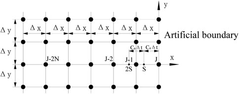
FIGURE 1. Discrete model of multi-transmitting boundary.

In Eq. 4, ${\mathit{c}}_{\mathit{a}}$ is the artificial wave velocity. The wave unilaterally travels at velocity $\mathit{c}$ and transmits in the direction of angle $\mathit{\theta }$ with a boundary surface (${\mathit{c}}_{\mathit{a}}=\mathit{c}/\mathit{cos}\mathit{\theta }$). As shown in Figure 1, Δx is the spatial step of the discrete grid in the direction perpendicular to the artificial boundary; Δt is the time step of the finite element calculation; and $\mathit{s}$ is a dimensionless parameter.

For first-order transmission (N=1), under the condition that Eq. 3 is satisfied, Eq. 1 can be written as follows:

${\mathit{u}}_{\mathit{J}}^{\mathit{P}+\mathbf{1}}=\left[{\mathit{t}}_{\mathbf{1}},{\mathit{t}}_{\mathbf{2}},{\mathit{t}}_{\mathbf{3}}\right]{\left[{\mathit{u}}_{\mathit{J}}^{\mathit{P}},{\mathit{u}}_{\mathit{J}-\mathbf{1}}^{\mathit{P}},{\mathit{u}}_{\mathit{J}-\mathbf{2}}^{\mathit{P}}\right]}^{\mathit{T}}(5)$

By substituting Eq. 4 into Eq. 5, the first-order MTF can be derived as

${\mathit{u}}_{\mathit{J}}^{\mathit{P}+\mathbf{1}}=\frac{\mathbf{1}}{\mathbf{2}}\left(\mathbf{1}-\mathit{s}\right)\left(\mathbf{2}-\mathit{s}\right){\mathit{u}}_{\mathit{J}}^{\mathit{P}}+\mathit{s}\left(\mathbf{2}-\mathit{s}\right){\mathit{u}}_{\mathit{J}-\mathbf{1}}^{\mathit{P}}+\frac{\mathbf{1}}{\mathbf{2}}\mathit{s}\left(\mathit{s}-\mathbf{1}\right){\mathit{u}}_{\mathit{J}-\mathbf{2}}^{\mathit{P}}(6)$

2.2 Analysis of the instability of high-frequency oscillations

The most intuitive explanation for high-frequency oscillation instability of MTF is the reflection amplification of high-frequency wave component in the artificial boundary. An amplification error wave is reflected to the artificial boundary in the finite calculation area and then amplified again, resulting in the instability of the artificial boundary. Such error wave amplification only occurs in high-frequency waves approaching the cut-off frequency. These high-frequency fluctuations causing oscillation instability are outside the scope of the frequency components considered in numerical simulation; and they do not benefit the computational stability of numerical simulation. In the numerical simulation, the high-frequency waves approaching the cut-off frequency have an insignificant effect on the accuracy of frequency bands. These high-frequency fluctuations exist perpendicular and parallel to the artificial boundary. Therefore, the elimination of useless high-frequency fluctuations in all directions can stabilize high-frequency oscillation without affecting the calculation accuracy.

2.3 Fundamental ideas of stabilization measures

In the meaningful frequency band of the finite element (or finite difference) simulation of the wave, the transmission boundary does not produce oscillation instability. Oscillation instability only occurs in the high-frequency band approaching the cut-off frequency. Therefore, the guiding principle of stabilization is to eliminate meaningless high-frequency components without affecting the low-frequency components meaningful for wave simulation.

In this paper, the proposed measure for suppressing oscillation instability is inspired by the concept of a multi-directional transmitting formula (Liao et al., 1993). The fundamental concept of the multi-direction transmitting formula is that the scattering wave from various directions radiates to the artificial boundary. This abandons the assumption that the scattering wave is based on a single direction and only uses the motion information of the node in the normal direction of the boundary. Instead, the transmission boundary formula is established using the motion information of all nodes adjacent to the artificial boundary node (including those on the artificial boundary and normal line).

The node position is shown in Figure 2 (I is the target node, and smooth filtering is performed using the nodes adjacent to point I on the boundary). When smoothing using three points, I, I − 1, and I + 1 are involved. When five points are used, I − 2, I − 1, I, I + 1, and I+2 are involved. In this regard, the following three considerations are emphasized.

1) Smoothing is performed after calculating the artificial boundary point at time P + 1.

2) Three or five points are selected to be used in smoothing; all points use their P + 1 values of time. For example, if the smoothing target point is I on the boundary, the participating points include point I on the boundary and the points adjacent to the boundary.

3) Smoothing is performed not only for displacement but also for the velocity values of the boundary point. This is implemented after calculating the displacement and velocity of the artificial boundary point at time P + 1.

FIGURE 2

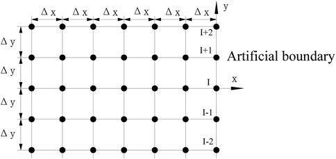
FIGURE 2. Position of the boundary point involvedin filtering.

After calculating the movement of the artificial boundary point at P + 1 using MTF (Eq. 1), the displacement and velocity values of the artificial boundary point I at P + 1 are smoothed. For point I on the boundary shown in Figure 2, three-point smoothing involves I − 1, I, and I + 1, and five-point smoothing involves I − 2, I − 1, I, I + 1, and I + 2. If three-point smoothing is used, the displacement and velocity can be calculated using Eqs 7, 9, respectively. If five-point smoothing is used, the displacement and velocity can be calculated using Eqs 8, 10, respectively. The displacement and velocity of point I after smoothing at P+1 are ${\stackrel{\sim }{\mathit{u}}}_{\mathit{i}}^{\mathit{P}+1}$ and ${\stackrel{\sim }{\dot{\mathit{u}}}}_{\mathit{i}}^{\mathit{P}+1}$, respectively. Coefficients β₁, β₂, and β₃ in Eqs 7, 9 are three-point smoothing coefficients, and coefficients β₁, β₂, β₃, β₄, and β₅ in Eqs 8, 10 are five-point smoothing coefficients. The values of the smoothing coefficients in Eqs 7–10 are presented in Section 2.4 of this paper.

${\stackrel{\sim }{\mathit{u}}}_{\mathit{i}}^{\mathit{P}+\mathbf{1}}={\mathit{\beta }}_{\mathbf{1}}{\mathit{u}}_{\mathit{i}}^{\mathit{P}+\mathbf{1}}+{\mathit{\beta }}_{\mathbf{2}}{\mathit{u}}_{\mathit{i}-\mathbf{1}}^{\mathit{P}+\mathbf{1}}+{\mathit{\beta }}_{\mathbf{3}}{\mathit{u}}_{\mathit{i}+\mathbf{1}}^{\mathit{P}+\mathbf{1}}(7)$

${\stackrel{\sim }{\mathit{u}}}_{\mathit{i}}^{\mathit{P}+\mathbf{1}}={\mathit{\beta }}_{\mathbf{1}}{\mathit{u}}_{\mathit{i}}^{\mathit{P}+\mathbf{1}}+{\mathit{\beta }}_{\mathbf{2}}{\mathit{u}}_{\mathit{i}-\mathbf{1}}^{\mathit{P}+\mathbf{1}}+{\mathit{\beta }}_{\mathbf{3}}{\mathit{u}}_{\mathit{i}+\mathbf{1}}^{\mathit{P}+\mathbf{1}}+{\mathit{\beta }}_{\mathbf{4}}{\mathit{u}}_{\mathit{i}-\mathbf{2}}^{\mathit{P}+\mathbf{1}}+{\mathit{\beta }}_{\mathbf{5}}{\mathit{u}}_{\mathit{i}+\mathbf{2}}^{\mathit{P}+\mathbf{1}}(8)$

${\stackrel{\sim }{\dot{\mathit{u}}}}_{\mathit{i}}^{\mathit{P}+\mathbf{1}}={\mathit{\beta }}_{\mathbf{1}}{\dot{\mathit{u}}}_{\mathit{i}}^{\mathit{P}+\mathbf{1}}+{\mathit{\beta }}_{\mathbf{2}}{\dot{\mathit{u}}}_{\mathit{i}-\mathbf{1}}^{\mathit{P}+\mathbf{1}}+{\mathit{\beta }}_{\mathbf{3}}{\dot{\mathit{u}}}_{\mathit{i}+\mathbf{1}}^{\mathit{P}+\mathbf{1}}(9)$

${\stackrel{\sim }{\dot{\mathit{u}}}}_{\mathit{i}}^{\mathit{P}+\mathbf{1}}={\mathit{\beta }}_{\mathbf{1}}{\dot{\mathit{u}}}_{\mathit{i}}^{\mathit{P}+\mathbf{1}}+{\mathit{\beta }}_{\mathbf{2}}{\dot{\mathit{u}}}_{\mathit{i}-\mathbf{1}}^{\mathit{P}+\mathbf{1}}+{\mathit{\beta }}_{\mathbf{3}}{\dot{\mathit{u}}}_{\mathit{i}+\mathbf{1}}^{\mathit{P}+\mathbf{1}}+{\mathit{\beta }}_{\mathbf{4}}{\dot{\mathit{u}}}_{\mathit{i}-\mathbf{2}}^{\mathit{P}+\mathbf{1}}+{\mathit{\beta }}_{\mathbf{5}}{\dot{\mathit{u}}}_{\mathit{i}+\mathbf{2}}^{\mathit{P}+\mathbf{1}}(10)$

2.4 Derivation of smoothing formula coefficient

For the foregoing smoothing formula, the key problem is the means for determining the value of the smoothing coefficient. The values of the smoothing coefficients are discussed as follows.

The relationship between the wavelength that may cause high-frequency instability at the boundary point and the mesh size of the finite element calculation is simplified into four cases, as shown in Figure 3.

FIGURE 3

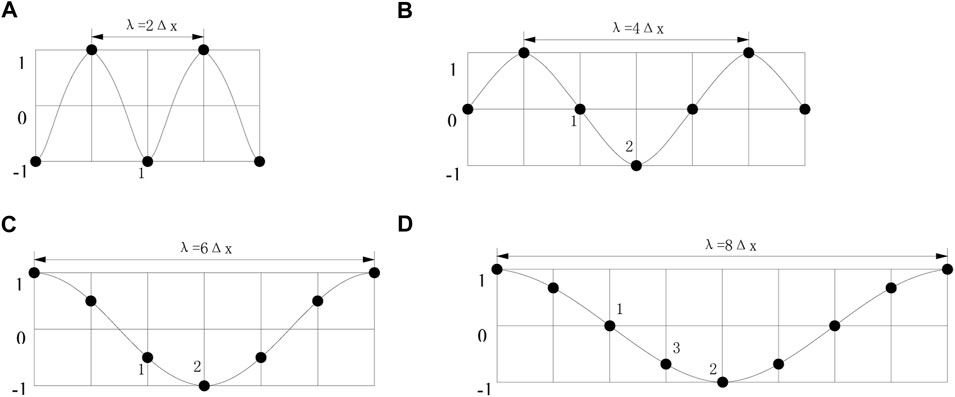
FIGURE 3. Wavelength and mesh size. (A) Wavelength and mesh size of case (a). (B) Wavelength and mesh size of case (b). (C) Wavelength and mesh size of case (c). (D) Wavelength and mesh size of case (d).

The smoothing effect of the coefficients considering four wavelengths shown in the figure is evaluated. Consider three-point smoothing as an example. The following four situations are discussed:

1) For case (a), the amplitude at point 1 in Figure 3A represents all points under the case. At point 1, the amplitudes before and after smoothing are −1 and ½ × (−1) + ¼ ×1 + ¼ × 1 = 0, respectively. The smoothed amplitude is found to be 0% of the original amplitude.

2) For case (b), the amplitudes at points 1 and 2 in Figure 3B represent those at all points. The amplitudes before and after smoothing at point 1 are 0 and ½ × 0 + ¼ × (−1) + ¼ × 1 = 0, respectively. The smoothed amplitude is found to be 0% of the original amplitude. At point 2, the amplitudes before and after smoothing are −1 and ½ × (−1) + ¼ × 0 + ¼ × 0 = −½, respectively. The smoothed amplitude is observed to be 50% of the original amplitude.

3) In case (c), the amplitudes at points 1 and 2 in Figure 3C represent those at all points in the case. At point 1, the amplitudes before and after smoothing are -1/2 and ½ × (−½) + ¼ × ½ + ¼ × (−1) = −3/8, respectively. The smoothed amplitude is observed to be 75% of the original amplitude. At point 2, the amplitudes before and after smoothing are −1 and ½ × (−1) + ¼× (−½) + ¼ × (−½) = −3/4, respectively. The smoothed amplitude is 75% of the original amplitude.

4) For case (d), the amplitudes at points 1, 2, and 3 in Figure 3D represent those at all points. At point 1, the amplitudes before and after smoothing are 0 and ½ × 0 + ¼ × ½ + ¼ × (−½) = 0, respectively. The smoothed amplitude is 0% of the original amplitude. At point 2, the amplitudes before and after smoothing are −1 and ½ × (−1) + ¼ × (−½) + ¼ × (−½) = −3/4, respectively. The smoothed amplitude is observed to be 75% of the original amplitude. At point 3, the amplitudes before and after smoothing are −½ and ½ × (−½) + ¼× 0 + ¼× (−1) = −½, respectively. The smoothed amplitude is 100% of the original amplitude.

Table 1 summarizes the smoothing values of using three coefficients in the four wavelength cases. The values in the table are amplitude percentages after smoothing relative to the original amplitude.

TABLE 1

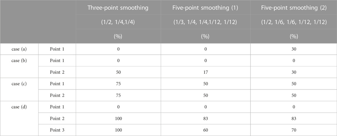
TABLE 1. Smoothed amplitude percentage.

With this filtering method, the amplitudes of the high-frequency and low-frequency waves are expected to decrease after smoothing. The foregoing eliminates meaningless high-frequency components without affecting the low-frequency part of the wave simulation. The percentage values corresponding to the calculation in this study after smoothing situations (a) and (b) are anticipated to be lower than those before smoothing. The percentage values after smoothing situations (c) and (d) must be higher than those before smoothing.

Table 1 indicates that the effect of values resulting from three-point smoothing is closest to that expected, followed by the effect of the five-point smoothing coefficient values (1/3, 1/4, 1/4, 1/12, and 1/12). The five-point smoothing coefficient values (1/2, 1/6, 1/6, 1/12, and 1/12) have the worst effect. Later, numerical tests are conducted to verify the effects.

3 Modified formula of the MTF with stabilization measure proposed

First-order and three-point smoothing are considered as an example to discuss the MTF after smoothing. With point I on the boundary shown in Figure 4 as the target point, three points, I, J, and R, on the boundary are involved in smoothing point I. According to Eq. 7, the motion expression of point I after smoothing at time P + 1 is.

${\stackrel{\sim }{\mathit{u}}}_{\mathit{I}}^{\mathit{P}+\mathbf{1}}={\mathit{\beta }}_{\mathbf{1}}{\mathit{u}}_{\mathit{I}}^{\mathit{P}+\mathbf{1}}+{\mathit{\beta }}_{\mathbf{2}}{\mathit{u}}_{\mathit{J}}^{\mathit{P}+\mathbf{1}}+{\mathit{\beta }}_{\mathbf{3}}{\mathit{u}}_{\mathit{R}}^{\mathit{P}+\mathbf{1}}(11)$

FIGURE 4

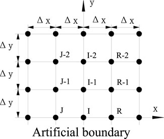
FIGURE 4. Discrete model of multi-transmitting boundary area.

According to Eq. 6, the motion expressions of I, J, and R at time P + 1 are Eqs 12–14, respectively:

${\mathit{u}}_{\mathit{I}}^{\mathit{P}+\mathbf{1}}=\frac{\mathbf{1}}{\mathbf{2}}\left(\mathbf{1}-\mathit{S}\right)\left(\mathbf{2}-\mathit{S}\right){\mathit{u}}_{\mathit{I}}^{\mathit{P}}+\mathit{S}\left(\mathbf{2}-\mathit{S}\right){\mathit{u}}_{\mathit{I}-\mathbf{1}}^{\mathit{P}}+\frac{\mathbf{1}}{\mathbf{2}}\mathit{S}\left(\mathit{S}-\mathbf{1}\right){\mathit{u}}_{\mathit{I}-\mathbf{2}}^{\mathit{P}}(12)$

${\mathit{u}}_{\mathit{J}}^{\mathit{P}+\mathbf{1}}=\frac{\mathbf{1}}{\mathbf{2}}\left(\mathbf{1}-\mathit{S}\right)\left(\mathbf{2}-\mathit{S}\right){\mathit{u}}_{\mathit{J}}^{\mathit{P}}+\mathit{S}\left(\mathbf{2}-\mathit{S}\right){\mathit{u}}_{\mathit{J}-\mathbf{1}}^{\mathit{P}}+\frac{\mathbf{1}}{\mathbf{2}}\mathit{S}\left(\mathit{S}-\mathbf{1}\right){\mathit{u}}_{\mathit{J}-\mathbf{2}}^{\mathit{P}}(13)$

${\mathit{u}}_{\mathit{R}}^{\mathit{P}+\mathbf{1}}=\frac{\mathbf{1}}{\mathbf{2}}\left(\mathbf{1}-\mathit{S}\right)\left(\mathbf{2}-\mathit{S}\right){\mathit{u}}_{\mathit{R}}^{\mathit{P}}+\mathit{S}\left(\mathbf{2}-\mathit{S}\right){\mathit{u}}_{\mathit{R}-\mathbf{1}}^{\mathit{P}}+\frac{\mathbf{1}}{\mathbf{2}}\mathit{S}\left(\mathit{S}-\mathbf{1}\right){\mathit{u}}_{\mathit{R}-\mathbf{2}}^{\mathit{P}}(14)$

By substituting Eqs 12–14 into Eq. 11, the motion expression of point I after smoothing at time P + 1 is derived as follows:

${\stackrel{\sim }{\mathit{u}}}_{\mathit{I}}^{\mathit{P}+\mathbf{1}}=\frac{\mathbf{1}}{\mathbf{2}}\left(\mathbf{1}-\mathit{S}\right)\left(\mathbf{2}-\mathit{S}\right)\left({\mathit{\beta }}_{\mathbf{1}}{\mathit{u}}_{\mathit{I}}^{\mathit{P}}+{\mathit{\beta }}_{\mathbf{2}}{\mathit{u}}_{\mathit{J}}^{\mathit{P}}+{\mathit{\beta }}_{\mathbf{3}}{\mathit{u}}_{\mathit{R}}^{\mathit{P}}\right)+\mathit{S}\left(\mathbf{2}-\mathit{S}\right)\left({\mathit{\beta }}_{\mathbf{1}}{\mathit{u}}_{\mathit{I}-\mathbf{1}}^{\mathit{P}}+{\mathit{\beta }}_{\mathbf{2}}{\mathit{u}}_{\mathit{J}-\mathbf{1}}^{\mathit{P}}+{\mathit{\beta }}_{\mathbf{3}}{\mathit{u}}_{\mathit{R}-\mathbf{1}}^{\mathit{P}}\right)+\frac{\mathbf{1}}{\mathbf{2}}\mathit{S}\left(\mathit{S}-\mathbf{1}\right)\left({\mathit{\beta }}_{\mathbf{1}}{\mathit{u}}_{\mathit{I}-\mathbf{2}}^{\mathit{P}}+{\mathit{\beta }}_{\mathbf{2}}{\mathit{u}}_{\mathit{J}-\mathbf{2}}^{\mathit{P}}+{\mathit{\beta }}_{\mathbf{3}}{\mathit{u}}_{\mathit{R}-\mathbf{2}}^{\mathit{P}}\right)(15)$

Eq. 15 can also be regarded as a multi-directional transmitting formula constructed using the information of all nodes (including I − 1, I − 2, J, J − 1, J − 2, R, R − 1, and R −2) around boundary node I, as shown in Figure 5. Coefficients β₁, β₂, and β₃ in Eq.15 can be considered as the share coefficients of node participation in transmission.

FIGURE 5

FIGURE 5. Multi-directional transmitting boundary.

Next, to verify the effectiveness of the proposed measure in suppressing high-frequency instability, numerical tests are conducted.

4 Numerical test

As an example, the wave propagation is simulated for a semi-infinite space model, as shown in Figure 6. The coordinates of the observation points are as follows: point 1 (0 m, 0 m); point 2 (−500 m, 0 m); point 3 (−500 m, −500 m); point 4 (−500 m, −1,000 m); point 5 (0 m, −1,000 m); and point 6 (0 m, −500 m). The input SH wave pulse–time history is shown in Figure 7. The incident angle is 0°, and the wave velocity is 2000 m/s. The mesh size is Δx = 10 m and Δy = 5 m. The calculated time step is Δt = 0.0025 s.

FIGURE 6

FIGURE 6. Calculation model.

FIGURE 7

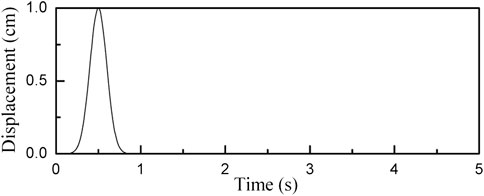
FIGURE 7. Displacement pulse.

Figure 8 shows the comparison results between implementing and not implementing the proposed measures for eliminating high-frequency instability. As shown in Figure 8, the coefficients are as follows: in three-point smoothing, β₁ = 1/2 and β₂ = β₃ = ¼; in five-point smoothing (1), β₁ = 1/3, β₂ = β₃ = ¼, and β₄ = β₅ =1/12; and in five-point smoothing (2), β₁ = 1/2, β₂ = β₃ = 1/6, and β₄ = β₅ =1/12.

FIGURE 8

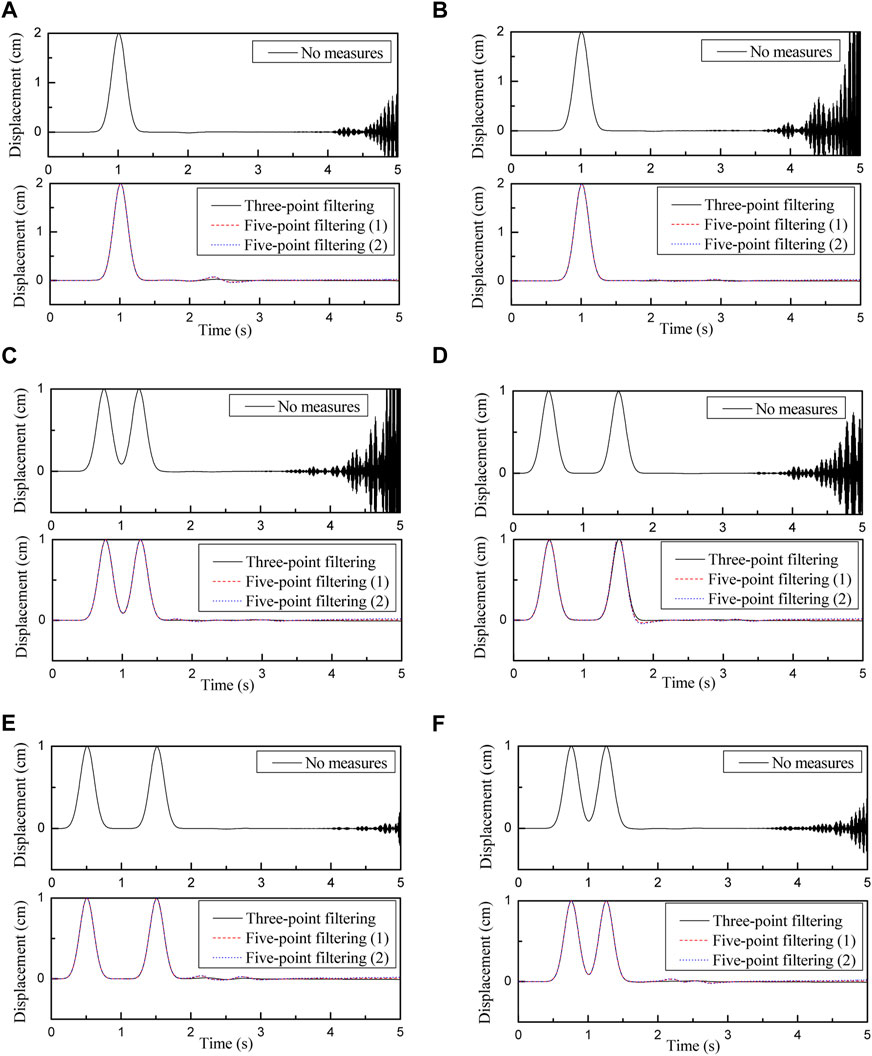
FIGURE 8. Displacement time history, (A) Observation point 1 (B) Observation point 2, (C) Observation point 3 (D) Observation point 4, (E) Observation point 5 (F) Observation point 6

By analysing the results of the displacement–time history comparison of observation points in Figure 8, the following are deduced.

1) The processing method of adjacent nodes participating in filtering smoothing on the artificial boundary is effective for suppressing the instability of high-frequency oscillations.

2) The corresponding curve of the three-point smoothing measure does not exhibit high-frequency oscillations, indicating that the measure has a satisfactory effect on suppressing high-frequency instability.

3) The time history curve of the observation point obtained using the five-point smoothing measure exhibits slight oscillations. Between the two values yielded by five-point smoothing, the following coefficients is the worst: 1/2, 1/6, 1/6, 1/12, and 1/12. In Figure 8B, C, E, the time history curves corresponding to the foregoing set of values have small high-frequency oscillations, indicating that this group of values cannot completely eliminate high-frequency instability.

4) In Figure 8E, F, the curves corresponding to the two five-point smoothing measures have distinct abnormal fluctuations between 2 and 3 s. No abnormal fluctuations are observed in the curves corresponding to those in which no measure for eliminating high-frequency oscillation is applied and the curves corresponding to the three-point smoothing measure. This shows that the abnormal fluctuation is caused by the disturbance from numerous low-frequency components introduced by the five-point smoothing method while filtering high-frequency components. The disturbance due to numerous low-frequency components causes abnormal fluctuations. This also demonstrates that the effect of the three-point smoothing measure is superior to that of the five-point smoothing one.

Table 2 lists the peak displacement–time histories of each observation point shown in Figure 8. The data in Table 2 indicate that the peak value of point 4 significantly differs. The peak value error obtained by the three-point smoothing measure is only 0.83%, whereas the errors obtained by the five-point smoothing one are 4.5% and 5.6%. This further demonstrates that three-point smoothing measure is better than five-point smoothing one. By considering the results in Figure 8; Table 2, the three-point smoothing measure is found to resolve the high-frequency instability, and the peak value of the observation point is least disturbed. This verifies the observation presented in Section 1.4. In terms of practical implementation, three-point smoothing is simpler than five-point smoothing. Accordingly, the use of the three-point smoothing measure is recommended.

TABLE 2

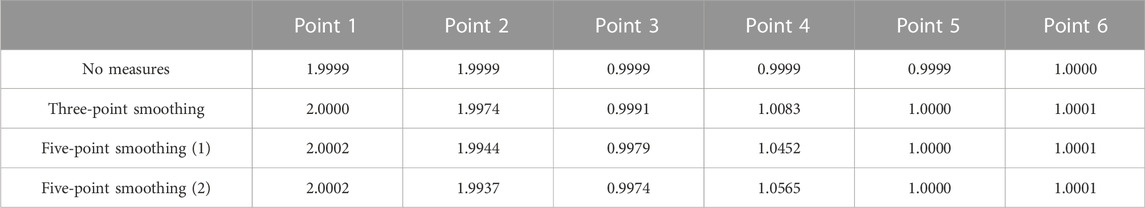
TABLE 2. Displacement peak of observation point.

5 Conclusion

Inspired by the multi-directional transmitting formula, and considering the high-frequency wave oscillation in the vertical and parallel directions with the artificial boundary, a strategy for filtering and smoothing adjacent nodes on the artificial boundary is proposed in this paper to suppress the instability of high-frequency oscillations of the multi-transmitting boundary. A reasonable smoothing coefficient value was obtained, and the effectiveness of the measure was verified through numerical tests. The main findings of the study are summarized as follows.

1) The smoothing filtering strategy using the adjacent nodes of the artificial boundary is effective in suppressing the instability of high-frequency oscillations of the multi-transmitting boundary.

2) This paper presents three types of smoothing coefficient value combinations. Both three-point and five-point smoothing measures are effective in suppressing high-frequency instability of the multi-transmitting boundary; however, the three-point smoothing measure exhibits better performance. This is because low-frequency components are inevitably introduced when high-frequency components are filtered. Five-point smoothing measure introduces more low-frequency interference factors than three-point smoothing one. Consequently, excessive low-frequency disturbances cause the time history curve to fluctuate and affect calculation accuracy.

3) This study analyses the conceptual similarity between the smoothing of the motion calculated by the boundary point and multi-directional transmitting formulas. Hence, it provides a reference for establishing the coefficient value of the multi-directional transmitting formula in the time domain.

Data availability statement

The original contributions presented in the study are included in the article/Supplementary Material, further inquiries can be directed to the corresponding author.

Author contributions

YY is the main author of this paper. XL made an important contribution to the innovation of this paper. MR and ZY gave good suggestions in the completion of the paper.

Funding

This study is supported by the National Natural Science Foundation of China (U1839202) and National Key Research and Development Program (2019YFB1900900).

Conflict of interest

The authors declare that the research was conducted in the absence of any commercial or financial relationships that could be construed as a potential conflict of interest.

Publisher’s note

All claims expressed in this article are solely those of the authors and do not necessarily represent those of their affiliated organizations, or those of the publisher, the editors and the reviewers. Any product that may be evaluated in this article, or claim that may be made by its manufacturer, is not guaranteed or endorsed by the publisher.

References

Cheng, N., and Cheng, C. H. (1995). Relationship between Liao and Clayton-Engquist absorbing boundary conditions: Acoustic case. Bull. Seismol. Soc. Am. 85 (3), 954–956. doi:10.1785/bssa0850030954

CrossRef Full Text | Google Scholar

Givoli, D. (1992). Numerical methods for problems in infinite domain. Amsterdam: Elsevier.

Google Scholar

Li, X. J., Liao, Z. P., and Du, X. L. (1992). An explicit finite difference method for viscoelastic dynamic problem. Earthq. Eng. Eng. Vib. 12 (4), 74–80. in Chinese.

Google Scholar

Li, X. J., and Tang, H. (2007). Numerical dissipation property of an explicit integration scheme for dynamic equation of structural system. Eng. Mech. 24 (2), 28–33. in Chinese.doi:10.1080/13632469.2017.1326423

CrossRef Full Text | Google Scholar

Li, X. J., and Yang, Y. (2012). Measure for stability of transmitting boundary. Chin. J. Geotechnical Eng. 34 (4), 641–645. in Chinese.doi:10.1371/journal.pone.0243979

CrossRef Full Text | Google Scholar

Liao, Z. P., and Liu, J. B. (1989). Finite element simulation of wave motion–basic problem and conceptual aspects. Earthq. Eng. Eng. Vib. 9 (4), 1–14. in Chinese.

Google Scholar

Liao, Z. P., and Liu, J. B. (1992). Fundamental problems in finite element simulation of wave motion. Sci. China (Series B) 34 (8), 874–882. in Chinese.

Google Scholar

Liao, Z. P., Zhou, Z. H., and ZhangY, H. (2002). Stable implementation of transmitting boundary in numerical simulation of wave motion. Chin. J. Geophys. 45 (4), 554–568. in Chinese. doi:10.1002/cjg2.269

CrossRef Full Text | Google Scholar

Liao, Z. P. (1984). A finite element method for near-field wave motion in heterogeneous materials. Earthq. Eng. Eng. Vib. 4 (2), 1–14. in Chinese.doi:10.1098/rspa.2016.0738

CrossRef Full Text | Google Scholar

Liao, Z. P. (2002). Introduction to wave motion theories in engineering. second edition. Beijing: Science Press. in Chinese.

Google Scholar

Liao, Z. P., and Wong, H. L. (1984). A transmitting boundary for the numerical simulation of elastic wave propagation. Soil Dyn. Earthq. Eng. 3, 174–183. doi:10.1016/0261-7277(84)90033-0

CrossRef Full Text | Google Scholar

Liao, Z. P., Wong, H. L., Yang, B., and Yuan, Y. (1984). A transmitting boundary for transient wave analyses. Sci. Sin. Ser. A. 27 (10), 1063–1076.doi:10.1360/YA1984-27-10-1063

CrossRef Full Text | Google Scholar

Liao, Z. P., and Yang, G. (1993). Multi-directional transmitting boundaries for steady-state SH waves. Earthq. Eng. Structrual Dyn. 24, 361–371. doi:10.1002/eqe.4290240305

CrossRef Full Text | Google Scholar

Tang, H., Li, X. J., and Li, Z. (2010). The effect of the explicit in tegration for defressing and eliminating the high- frequency instability induced by local transmitting boundary. World Earthq. Eng. 26 (4), 50–54. in Chinese.doi:10.1007/BF02650573

CrossRef Full Text | Google Scholar

Wolf, P., and Song, C. (1996). Finite-element modelling of unbounded media. Chichester: John Wiley & Sons.

Google Scholar

Wolf, P. (1988). Soil-structure dynamic interaction analysis in time domain. Englewood Cliffs, NJ: Prentice-Hall.

Google Scholar

Xie, Z. N., and Liao, Z. P. (2012). Mechanism of high frequency instability caused by transmitting boundary and method of its elimination—SH wave. Chin. J. Theor. Appl. Mech. 44 (4), 745–752. in Chinese.doi:10.6052/0459-1879-11-312

CrossRef Full Text | Google Scholar

Xing, H. J., and Li, H. J. (2017a). Implementation of multi- transmitting boundary condition for wave motion simulation by spectral element method: One dimension case. Chin. J. Theor. Appl. Mech. 49 (2), 367–379. in Chinese.doi:10.6052/0459-1879-16-393

CrossRef Full Text | Google Scholar

Xing, H. J., and Li, H. J. (2017b). Implementation of multi- transmitting boundary condition for wave motion simulation by spectral element method: Two dimension case. Chin. J. Theor. Appl. Mech. 49 (4), 894–906. in Chinese.doi:10.6052/0459-1879-16-393

CrossRef Full Text | Google Scholar

Xing, H. J., Li, X. J., Liu, A. W., Li, H. J., Zhou, Z. H., and Chen, S. (2021). Extrapolation-type artificial boundary conditions in the numerical simulation of wave motion. Chin. J. Theor. Appl. Mech. 53 (5), 1480–1495. in Chinese.

Google Scholar

Xu, S. G., and Liu, Y. (2018). 3D acoustic and elastic VTI modeling with optimal finite-difference schemes and hybrid absorbing boundary conditions. Chin. J. Geophys. 61 (7), 2950–2968. in Chinese.doi:10.6038/cjg2018L0250

CrossRef Full Text | Google Scholar

Yang, Y., Li, X. J., He, Q. M., and Wang, L. (2014). Comparison of measures for eliminating high-frequency instability of a multi-transmitting boundary in scattering problems. China Earthq. Eng. J. 36 (3), 476–481. in Chinese.doi:10.1002/cnm.1394

CrossRef Full Text | Google Scholar

Zhang, X. B., Liao, Z. P., and Xie, Z. N. (2021). Mechanism of high frequency instability and stable implementation for transmitting boundary—P-SV wave motion. Chin. J. Geophys. 64 (10), 3646–3656. in Chinese.doi:10.6052/0459-1879-11-312

CrossRef Full Text | Google Scholar