 Shen Jirong1
 Chen Shaolin
- 1College of Aerospace Engineering, Nanjing University of Aeronautics and Astronautics, Nanjing, China
- 2College of Civil Aviation, Nanjing University of Aeronautics and Astronautics, Nanjing, China
The simulation of seismic wave propagation in marine areas, which belongs to seismoacoustic scattering problem, is complicated due to the fluid-solid interaction between seawater and seabed, especially when the seabed is saturated with fluid. Meanwhile, huge computation resources are required for large-scale marine seismic wave simulation. In the paper, an efficient parallel simulation code is developed to solve the near-field seismoacoustic scattering problem. The method and technologies used in this code includes: 1) Unified framework for acoustic-solid-poroelastic interaction analysis, in which seawater and dry bedrock are considered as generalized saturated porous media with porosity equals to one and zero, respectively, and the coupling between seawater, saturated seabed and dry bedrock can be analyzed in the unified framework of generalized saturated porous media and avoid interaction between solvers of different differential equation; 2) Element-by-element strategy and voxel finite-element method (VFEM), with these strategies, it only needs to calculate several classes of element matrix and avoid assembling and storing the global system matrices, which significantly reduces the amount of memory required; 3) Domain-partitioning procedure and parallel computation technology, it performs 3D and 2D model partitioning for the 3D and 2D codes respectively, sets up the velocity structure model for the partitioned domain on each CPU or CPU core, and calculates the seismic wave propagation in the domain using Message Passing Interface data communication at each time step; 4) Local transmitting boundary condition, we adopt multi-transmitting formula, which is independent of specific wave equations, to minimize reflections from the boundaries of the computational model. A horizontal layered model with the plane P-wave incident vertically from bottom is used to demonstrate the computational efficiency and accuracy of our code. Then, the code is used to simulate the wave propagation in Tokyo Bay. All codes were written following to the standards of Fortran 95.
1 Introduction
With the increasing exploitation and utilization of marine resources, a large number of marine engineering structures and infrastructures, such as oil platforms, cross-sea bridges, submarine tunnels, and artificial islands, have been constructed. In order to ensure the safety of these offshore structures under the action of earthquake, it is necessary to accurately predict the ground motion of the sea area. Currently, there are mainly three categories of ground motion predictions, which are known as prediction based on the attenuation relationship of ground motion, theoretical analysis prediction and numerical simulation prediction. For the prediction based on the attenuation relationship of ground motion, fewer offshore strong-motion records are gathered than the onshore strong-motion records, coupled with the lack of material parameters and spatial distribution of marine soil layers, which makes it difficult to determine the attenuation relationship of marine ground motions. Consequently, onshore strong-motion records are commonly selected for the seismic design of offshore structures. However, Nakamura et al. (2014) investigated the seismic wave amplification in and around the Kii peninsula using observation data analyses and numerical simulations from land (K-net) and seafloor stations (DONET), and the results indicate that the amplifications at the marine sites with low-velocity sediment layers partially contribute to an overestimation of magnitude, if the same empirical equations as those used for data observed at land stations are applied without any correction allowed for seismic amplification caused by ocean-specific structures. Similarly, Hu et al. (2020) pointed out that the seismic attenuation relationship of offshore site is significantly different from that of onshore site due to the deep soft sediment layer. For the theoretical analysis prediction, many researchers have simplified the sea area terrain into a regular model, and solved the marine ground motion response by theoretical methods (Brekhovskikh, 1980; Zhu, 1988; Okamoto and Takenaka, 1999; Li et al., 2017; Ke et al., 2019). However, this kind of method can only be applied to sites with regular terrain (such as horizontally layered sites), and cannot be directly used for ground motion simulation of offshore sites with complex terrain.
With the development of computer technology and the maturity of numerical calculation methods, some researchers have begun to use numerical simulation methods to solve the ground motion response of complex sea areas in the last few decades. Morency and Tromp (2008) based upon domain decomposition, described wave propagation in different media and discussed the interfacial continuity conditions used to deal with the discontinuities between different media. Link et al. (2009) deduced the 2D finite element format of fluid-solid-acoustic field interaction. Nakamura et al. (2012) simulated ground motions in the Suruga Bay, and the results showed that the seawater layer and the irregular topography of the sea area have a significant impact on the amplitude and duration to the coda part of S-wave. Liu et al. (2019) simulated the wave radiation effect of infinite fluid and solid domains on the reef-seawater system through the corresponding artificial boundary conditions. In the above numerical methods, fluid, solid, and poroelastic medium are analyzed by independent solvers, and then mutual interfacial coupling is performed through data exchange, which is very inconvenient. Chen et al. (2019a) and Chen et al. (2019b) proposed a decoupling simulation technique to model seismoacoustic scattering in marine areas when a seismic wave is incident. Different media (fluid, saturated porous medium, solid) are successfully unified into the generalized saturated porous media framework by extending Biot’s saturated porous media theory and continuous conditions between different media. In the unified framework, different media can be simulated simultaneously in a single solver by assigning the corresponding parameters (porosity, wave velocity, density, etc.) to generalized saturated porous media.
Although researchers have proposed many methods to simulate the seismoacoustic scattering of marine sites, the ground motion simulation of 3D large-scale sea areas is still limited by computer hardware and computing time. In the exiting research, only the long period (T > 2 s) synthetic waveforms fit well with the observed waveforms (Nakamura et al., 2015; Okamoto et al., 2017; Takemura et al., 2019; Oba et al., 2020; Takemura et al., 2021). Therefore, it is necessary to build high-resolution models for broadband marine wave propagation simulation. In addition, previous studies have shown that 3D oceanographic models can simulate seafloor ground motion more accurately than 1D/2D models, especially in areas with drastic topographic changes (Takemura et al., 2020; Wang and Zhan, 2020; Bao et al., 2022). Compared with the 1D/2D model, if the 3D model is used to simulate the seismoacoustic scattering in marine areas with high spatial resolution, the demand of computational resources increases rapidly, and the traditional calculation can no longer meet the calculation requirements. In order to improve computing efficiency and make full use of computer performance, Okamoto et al. (2010), Liu et al. (2017), and Maeda et al. (2017) used GPU parallelism, CPU master-slave communication parallelism, and CPU cache communication parallelism to accelerate the simulation of ground motions for 3D sites, respectively.
Compared with numerical methods that use a structured grid, FEM with an unstructured grid has a greater capability of analyzing a body with complicated configuration. However, using FEM to simulating wave propagation in models constructed by irregular computational grids requires vast amounts of computational resources for computing stiffness matrix. In addition, the model discretization by 3D unstructured elements is often laborious (Ho-Le 1988). A so-called voxel finite-element method (VFEM) has been proposed to resolve these difficulties of FEM with an unstructured grid (Koketsu et al., 2004), which avoids generating distorted elements. In addition, the combination of VFEM and EBE method can significantly reduce the demand for computational memory and improves the robustness of computing.
In this study, a new VFEM simulation code based on unified framework and parallel computational strategy is developed to realize high performance computing for marine acoustics and submarine earthquake in the 2D/3D marine field. The unified framework of generalized porous media is applied to simulate the fluid-solid interaction in marine areas (Chen et al., 2019a; Chen et al., 2019b), which avoid exchanging the interfacial response between different solvers. In addition, parallel technology is also used to improve the computing efficiency. The large-scale site is divided into several small models, and the wave propagation simulation of each small model is assigned to each CPUs. The coupling between different CPUs is realized by Message Passing Interface (MPI) data communication at each time step.
In the following, we briefly review the strategy of the generalized saturated porous media framework in Section 2. In Section 3, the numerical techniques adopted in the present code are described, and a 3D horizontal layered field with the plane P-wave input vertically from bottom is used for the benchmark test of our code. Finally, in Section 4, the seismoacoustic scattering simulation in the Tokyo Bay with the vertically incident plane P/SV wave is performed by our code.
2 Methods
In this section, we briefly introduce the FEM based on unified computational framework for simulating wave motion in water-saturated seabed-bedrock system and the algorithms adopted in our code. The details of theories can be found in Chen et al. (2003, 2019a, 2019b).
2.1 Mathematical model of generalized saturated porous media dynamics
Theoretically, solid and fluid media are special cases of saturated porous media with porosity of 0 and 1, respectively, and the coupling between different media can all be described in the generalized saturated porous media system.
2.1.1 Basic differential equation
According to Biot porous medium theory, the vector representation of the basic differential equations of the model are given as follows (Biot 1956; 1962):
Solid-phase equilibrium equation for saturated porous media
Liquid-phase equilibrium equation for saturated porous media
Compatibility equation (considering initial pore pressure and initial body strain as zero)
Where
Assuming
2.1.2 Continuity conditions of the interface
The relationship between two kinds of saturated porous media (
Hereafter, the term containing subscript N represents the normal component of the vector, and the term containing subscript T represents the tangential component of the vector. The terms with and without the dash at the top represent the physical quantities corresponding to the material on one side of the interface and the material on the other side, respectively. Assuming
and extend the continuity conditions for saturated porous media-saturated porous media interface to that for generalized saturated porous media-generalized saturated porous media interface, which can be described by Eqs 6, 7, 11 ∼ Eq. 13.
By assigning the corresponding values of saturated porous media as parameters of solid or fluid, the continuity conditions of four special interfaces (i.e., fluid-saturated porous medium, saturated porous medium-solid, fluid-solid, saturated porous medium-saturated porous medium), can be unified into the continuity conditions between two generalized saturated porous media.
2.1.3 Boundary conditions
The boundary conditions consist of Dirichlet boundary condition, Neumann boundary condition and artificial boundary condition. As above, we extend the boundary conditions of saturated porous media to that of the generalized saturated porous media, Dirichlet boundary condition and Neumann boundary condition may be expressed as:
Dirichlet boundary condition
Neumann boundary condition
where
For the fluid,
2.2 Discretization and solution of motion equations
Take a random node as an example, using the Galerkin method to discretize Eqs 1, 2, and considering the boundary conditions, the decoupling motion equilibrium equation of any node i can be obtained as [Chen et al. (2019)]:
where
2.2.1 Internal node
For the internal nodes,
where
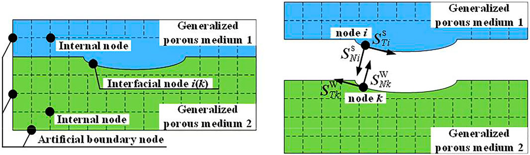
FIGURE 1. Schematic diagram of interfacial force.
2.2.2 Interfacial node
Here we discuss the situation where node i k) is the interfacial point between two different media, which is shown in Figure 1. Using the concept of isolator, and performing time-step integration on Eqs 18, 19 at time
where
where
After obtaining
With the interfacial force, the displacement response of the interfacial node can be solved by Eqs 22, 23.
2.2.3 Boundary node
In order to effectively simulate the motion of the outgoing wave across the artificial boundary, we use the Multi-Transmitting Formula (MTF) proposed by Liao et al. (1984):
where
This local artificial boundary condition is universal and has nothing to do with specific wave equations, which can be directly used for wave problems in saturated porous media (Liao et al., 1984; Chen and Liao, 2003). The total displacements
In which
3 Software implementations
Based on the unified framework and the algorithms mentioned before, we developed a new code for simulating wave propagation in large-scale marine site. This code is especially designed to improve usability for non-expert users who are not familiar with numerical simulation techniques. Thus, this code also adds pre-processing and partial post-processing functions, and integrates codes between different modules through Linux script files. Users do not need to modify the code to apply it to individual simulation targets, but only needs to input the corresponding control parameters and soil layer elevation, and then the process of finite element model establishment—free field calculation—finite element simulation can be realized automatically (Figure 2).
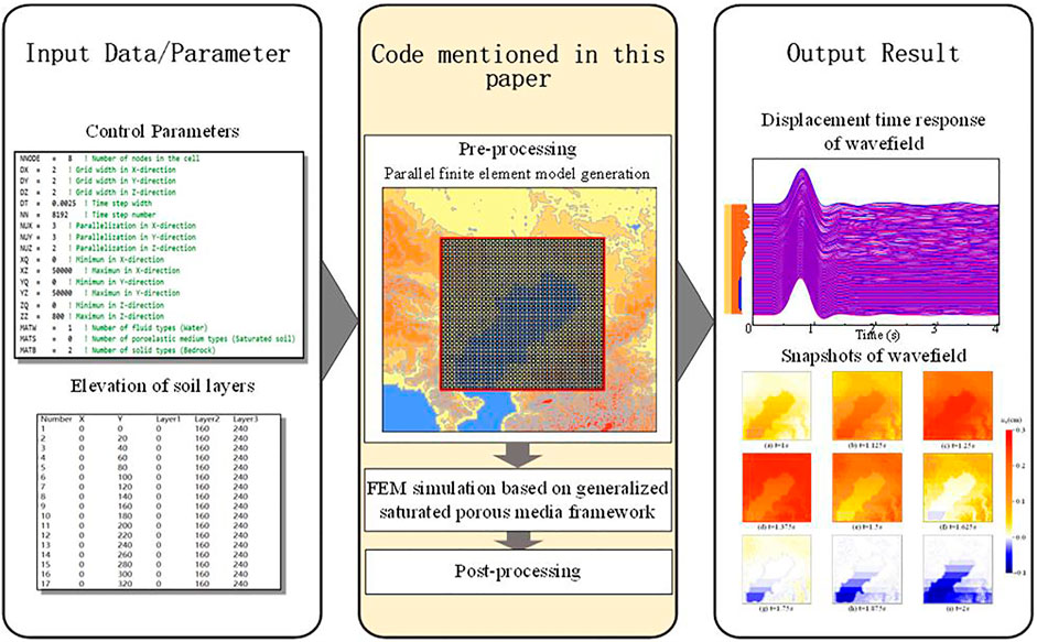
FIGURE 2. A schematic illustration of the flow of the wave propagation simulation using the code presented in this paper [Reproduced from Figure 1 of Takuto et al. (2017) with modification].
3.1 Establishment and discretization of finite element model
Based on the comprehensive overview of geological data and borehole data, the marine site is assumed as a layered model consisting of basements and sedimentary layers. The P-wave velocities to the basements and sedimentary layers are measured by refraction and reflection surveys, the S-wave velocities are obtained by borehole logging, microtremor surveys or the empirical relationships between P- and S-wave velocities, and the density of layers is obtained by borehole logging. After that, convert time sections from seismic reflection surveys and borehole logging into depth sections using the P- and S-wave velocities. Depth sections are spatially combined with borehole data to produce the 3D model via interpolation, such as Bicubic spline interpolation and Kriging interpolation. Then the depth and material parameters of each soil layer can be input into our code for finite element mesh generation and subsequent marine seismoacoustic scattering simulation.
FEM can handle very complex structures with high accuracy using elements with various shapes. However, the pre-processing of FEM, i.e., grid generation, can be very time-consuming. In order to overcome the limitation of FEM, we use voxel FEM (VFEM). “Voxel” is a term in computer graphics derived from an abbreviation of “volume pixel.” It is actually a hexahedron or rectangular prism in three dimensions and its cross section forms a pixel in two dimensions (Koketsu et al., 2004). In our code, by reading the site information (such as material parameters of soil layer, elevation, etc.) and element size input by the user, the model is discretized into regular hexahedral elements, and the corresponding material parameters are assigned. The directional derivatives at the interface of different media (fluid, saturated porous medium, solid) are also calculated and stored for subsequent finite element calculations. It is noted that the approximate treatment of a smooth boundary using voxels can lead to errors in computing displacement, and the errors become larger as the shape of the boundary becomes more irregular, but the computational accuracy requirements can generally be met by refining the mesh. VFEM mesh generation is simple and fast, and avoids generating distorted elements. Moreover, VFEM reduces the requirements of computational resources and memory.
3.2 Element-by-element and parallel computing strategy
The simulation of wave propagation in large-scale sea fields usually requires a large amount of memory and has a heavy computational load. The key to large-scale marine seismoacoustic scattering simulation is to realize the high-performance computing and save computational memory. In conventional finite element calculations, the global system matrices (including mass matrix, damping matrix, stiffness matrix etc.) usually needs to be assembled, which leads to a considerable increase in the memory usage for large-scale simulation. Therefore, the element-by-element (EBE) method is adopted in our code. It is only necessary to classify elements based on their material and size, and then calculate the mass matrix, damping matrix, and stiffness matrix for each class of elements before the solution begins, avoid assembling and storing the global system matrices. The combination of VFEM and EBE method can significantly reduce the demand for computational memory, which is suitable for large-scale marine seismoacoustic scattering simulation. When calculating the response of each node, it is only necessary to obtain the constitutive force of the node through the stiffness matrix and damping matrix of the elements around the node, and obtain the response of the node through the lumped mass and explicit integration scheme, which can avoid solving large system of equations and have high computational efficiency.
Our code also adopts a domain-partitioning procedure for the parallel computing using MPI. It performs 3D and 2D model partitioning for the 3D and 2D codes. The finite element model of each partitioned domain is set up on each CPU or CPU core, and the seismic wave propagation is calculated using MPI data communication at each time step. To ensure the continuity of the waveform across the partitioned model, the displacement and force defined at the outermost node are exchanged with those of the neighboring partitioned models at each time step using MPI.
3.3 Seismic source and input
Depending on the relative location of the model and the seismic source, the wave propagation problem can be divided into two categories: inner-source problem and scattering problem. For the inner-source problem, the seismic source is contained within the computational region. The finite fault source can be represented by multiple point sources, and the seismic input can be imposed at the corresponding nodes of the model. For scattering problem, that is the case for the plane wave incidence, the seismic input is realized through free-field response (see Section 2.2.3). When the boundary of the computational model can be simplified to a horizontally layered region, the free field response can be obtained directly by the transfer matrix method (Ke et al., 2019). However, when the topography at the boundary of the model is irregular, as shown in Figure 3, we need to first develop a finite element model for the 1D column that has the same mesh density as the corner of 3D model, then obtain the response of the 1D corner column model by the transfer matrix method. After that, establish a 2D finite element model with the same mesh density as the 3D model at the cut-off boundaries, input the 1D response into the 2D model as the free field and simulate the wave propagation in 2D model, then take the 2D FEM synthetic wave field as “free fleid” and input it into the 3D model through the artificial boundary condition, as mentioned in Section 2.2.3.
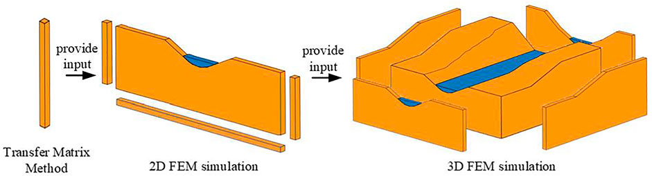
FIGURE 3. Flow chart for simulating wave propagation in 3D model with irregular boundary (Reproduced from figure 4.2 of Lokke (2019) with modification).
In order to provide free field response for the 3D model with irregular boundaries, a code for the 2D-VFEM simulation with the incident P/SV wave is also included in our code. The 2D-VFEM simulations use the same input parameter file, except they perform the wave propagation simulations in the x–z plane, users can switch between 2D-VFEM and 3D-VFEM simulation or choose the wave motion input mode applicable to individual targets by simply setting corresponding input parameters without modifying the code, which is user friendly.
3.4 Computation performance
The computational efficiency and accuracy of the parallel simulation was examined using the following numerical test. The model used in the test is a 36-m bedrock covered with 30-m seawater (Figure 4A), and a plane P-wave with a pulse duration of .15 s (Figures 4B, C) is input from the bottom of the bedrock. The expression of the incident P-wave is:
where W is the pulse duration. The time increment
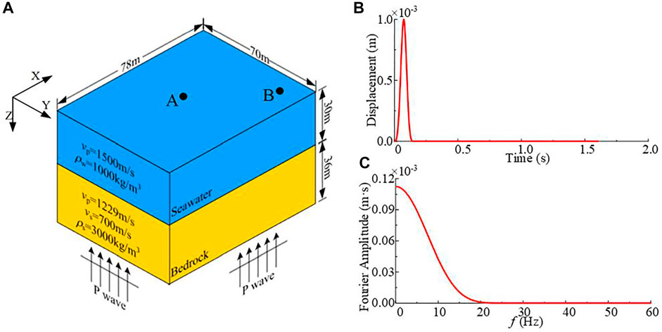
FIGURE 4. The computational model and the input pulse wave (A) Schematic diagram of horizontal layered computational model; (B) Displacement time history of the input wave; (C) Displacement Fourier amplitude spectrum of the input wave.
To illustrate the calculation accuracy of our code, the displacement time history of two monitoring points (point A, B, as shown in Figure 4A) in the above case simulated by our code, together with analytical solution obtained by the transfer matrix method, are plotted in Figure 5. The responses obtained by our code agree well with those obtained by the transfer matrix method.
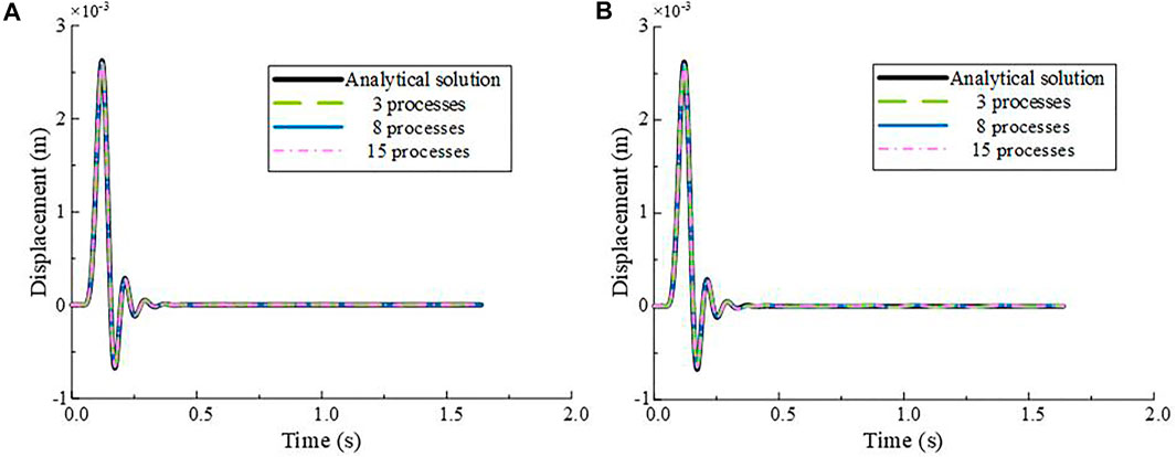
FIGURE 5. Displacement time history calculated by our code using different numbers of CPUs: (A) Point A; (B) Point B.
Figure 6 shows the curve for calculating efficiency of our code. For the element-by-element parallel VFEM, at least two processes are required for parallel computation, assuming that the total computational time spent with 2 processes is t2, and the theoretical computational time with m processes is defined as tm=2 × t2/m. The curve demonstrates that as the number of processes increases, the computational time spent on the 3D simulation code decreases. However, when the number of processes reaches 14 or more, the computation time consumption almost does not decrease, and the gap between the theoretical computing time consumption and the actual computation time consumption increases gradually. This is due to the large number of processes used for small model simulation, the data traffic between different regions increase dramatically and resulting in over parallelization.
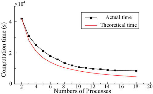
FIGURE 6. Calculation efficiency curve.
4 Simulation case
To demonstrate the effectiveness of our code in seismic wave propagation simulations, here we choose Tokyo Bay as the site model, and the scope of the study area is shown in Figure 7A (black frame line). The horizontal dimension of the model is 50 km × 50 km and the depth is .8 km, and artificial boundaries are applied at the boundaries of the model for absorbing the outgoing waves. It can be seen from Figure 7A that the topographic changes rapidly in the southeast of Tokyo Bay, and the rest of the area is relatively flat (the topography of the land surface and the seabed was obtained from Google Earth).
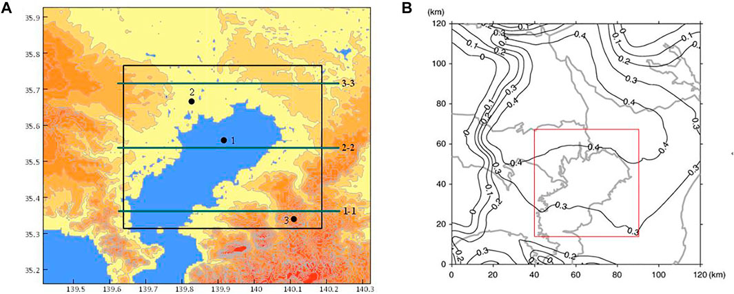
FIGURE 7. (A) Topography of the area around Tokyo Bay; (B) The first interface depth determined by Koketsu et al. (2009).
Koketsu et al. (2009) divided the soil layers in the vicinity of Tokyo Bay into four categories according to the wave speed and density, and gave the parameters of each soil layer and the depth of each interface within a range of 120 km × 120 km. According to Koketsu et al. (2009), the depth range of the first interface is 0–0.4 km (Figure 7B), and the depth of the second interface is greater than 1 km. Thus, two categories of soil layers and one interface are contained in the computational model here. Since the detailed interface depth is difficult to obtain, it can be seen from Figure 7B that the depth of the first interface is about .2–.4 km in the simulation region (red frame line), and gradually becomes deeper from south to north. Here we simplify the depth of the interface from south to north as a linear increase from 260 to 400 m.
Assuming that the model is only composed of seawater and elastic bedrock, and the material parameters are given in Table 1.
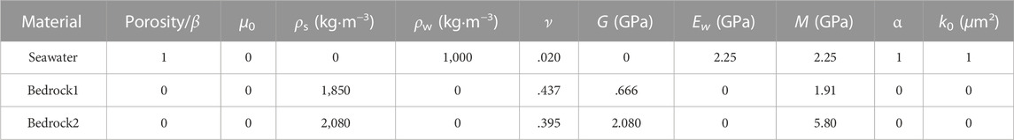
TABLE 1. Parameters of materials used in Tokyo Bay (Koketsu et al., 2009).
A plane P/SV wave with a rise time of 20 s is input from the bottom of the bedrock, and its expression is consistent with the incident wave in Section 3.4 (Eq. 36) but setting the pulse duration W = 1 s. The displacement time history, acceleration time history and corresponding Fourier spectrum of the incident wave are shown in Figure 8.
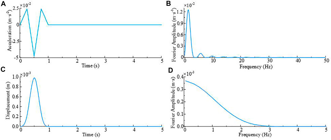
FIGURE 8. Input pulse wave: (A) Acceleration time history; (B) Acceleration Fourier amplitude spectrum; (C) Displacement time history; (D) Displacement Fourier amplitude spectrum.
The simulation model has a grid spacing of 20 m and a time step of .0025 s with the minimum wave speed of 0.6 km/s for the shallow-most bedrock layer, which meets the requirements of numerical stability and accuracy. The model is divided into 144 domains, each domain has about 1.7 million elements, and the number of elements of the whole model is about 250 million.
Three cases are performed by our code: Case1, the seismoacoustic scattering simulation of Tokyo Bay with plane P-wave incidence; Case2, similar to case 1 but without seawater layer; Case 3, the seismoacoustic scattering simulation of Tokyo Bay with plane SV-wave incidence. In all three cases, 64 CPUs are used to simulate wave propagation in the field, and take an average of 38 h to complete the calculation. Three points shown in Figure 7A are selected as observation points, which are located on the bottom of the sea (point 1), the plain (point 2), and the top of the mountain (point 3), respectively. At the same time, three cross sections shown in Figure 7A are selected to monitor the displacement wave field at the top of the bedrock.
4.1 Plane P-wave input
The displacement time history, acceleration time history and acceleration Fourier spectrum of each observation point are shown in Figure 9. When the P-wave is vertically incident from the bottom of the model, the displacement of the three observation points in the z-direction is much larger than that in the other two directions. The reflection of the incident wave between different media can be clearly observed, and the arrival time of the first displacement peak is also delayed with increasing altitude. In addition, affected by the surrounding complex terrain, the response of point 3 in the horizontal direction is more intense than that of other two points. While points 1 and 2 are in regions with slow elevation changes, and these two points are similar in terms of displacement time history, acceleration time history, and Fourier spectrum.
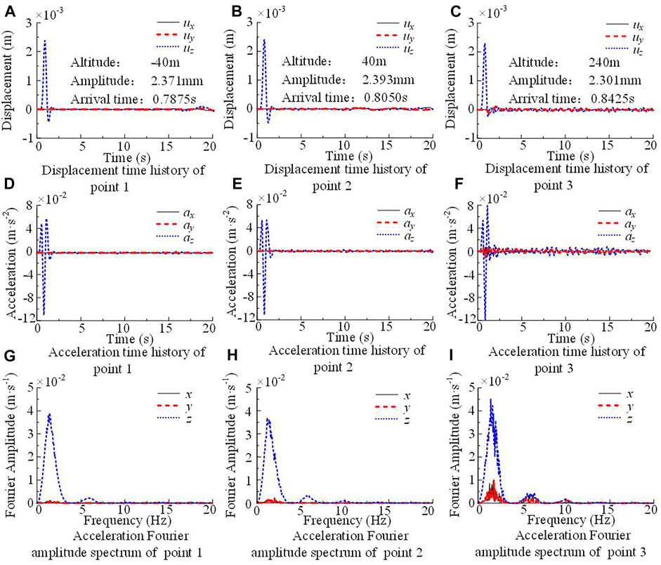
FIGURE 9. Displacement, acceleration time history curve and acceleration Fourier spectrum of observation points with P-wave input.
Figure 10 illustrates the displacement time response along the top of bedrock1 of different cross sections. When the P-wave is vertically incident, the ground motions are mainly controlled by the vertical component. Section 1-1 contains both marine area and mountain area. For the marine area, the terrain is relatively flat, which makes the vertical displacements in this area stable rapidly after the end of the major response. However, in the mountainous area with drastic elevation changes, the incident wave scattered when it reaches the free surface, and the scattering waves propagate back and forth in the irregular region, triggering the complex subsequent waveforms (Figure 10A). Since the topography changes slowly in both sections 2-2 and 3-3, the peak vertical displacements as well as their arrival times are relatively coincident, and the scattering of the waves is only observed near regions with topographic change.
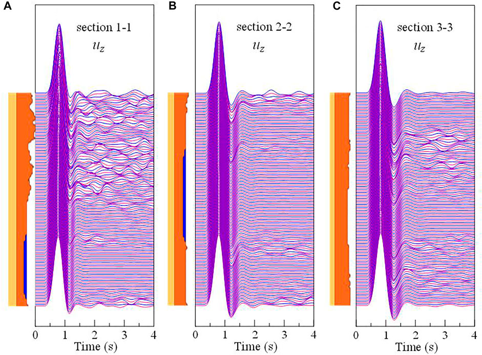
FIGURE 10. (A) Displacement waveforms in z-direction of section 1-1; (B) Displacement waveforms in z-direction of section 2-2; (C) Displacement waveforms in z-direction of section 3-3.
The snapshots of the displacement wavefield at the top of the bedrock layer are shown in Figure 11. As time going on, the incident wave first reaches the seafloor where the bedrock is the thinnest, then gradually spreads over the land, and finally reaches the mountainous area with high altitude. Furthermore, as mentioned earlier, the depth of the interface between bedrock 1 and bedrock 2 is simplified to south-to-north increasing, which means that the thickness of bedrock 2 gradually increases from north to south. Since the wave speed of bedrock 2 is greater than that of bedrock 1, the arrival time of incident wave is gradually advanced from north to south in areas with similar elevations.
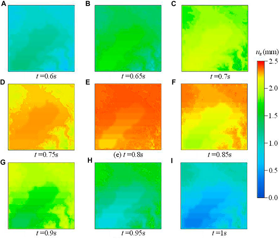
FIGURE 11. The snapshots of the displacement wavefield with P-wave input.
The synthetic results without seawater layer are plotted in Figure 12 together with the results with seawater layer. Owing to the shallow depth of the seawater, the difference between the two cases is small, especially in the regions far from the marine area. Even so, in the offshore area, slight differences can be observed in areas where the terrain changes rapidly (Figure 12A). The displacement time history of point 1 is shown in Figure 12B for further comparison of the two cases. Since P waves can propagate in the seawater layer, the arrival time of incident wave with the seawater layer (red line in Figure 12B) is slightly later than that without the seawater layer (green line in Figure 12B). In addition, seawater acts as a “filler” on the seabed and weakens the influence of irregular terrain on the waveform, which makes the coda relatively stable.
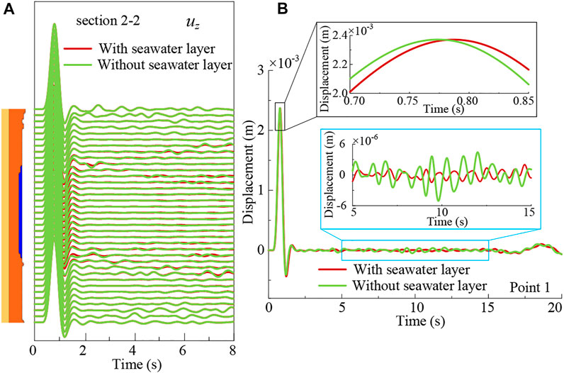
FIGURE 12. Comparison of the cases with and without sea water layer: (A) Displacement waveforms along the top of bedrock layer of cross section 2-2; (B) Displacement time history of point 1
It is worth mentioned that when our code is applied to simulating the wave propagation in the example without seawater, only need to set the material parameters of seawater such as compressive modulus and density to zero without modifying the model, which is very convenient.
4.2 Plane SV-wave input
The displacement time history, acceleration time history and acceleration Fourier spectrum of each observation point are shown in Figure 13. Similar to the case of P-wave incidence, the arrival time of the incident wave is also delayed with increasing altitude, and the ground motions are mainly controlled by the motion direction of the incident wave, here is the x-direction. The displacement time history of point 1 is relatively stable after 10 s, but the acceleration of point A in the z-direction has obvious oscillations (Figure 13D), which does not appear in the case of P-wave incidence. Since the material is assumed to be linear elastic here, the spectral characteristics of the output acceleration Fourier spectrum remain consistent with the input regardless of the terrain.
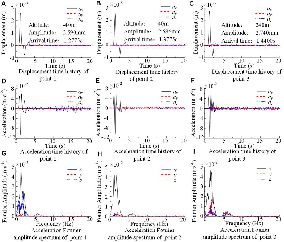
FIGURE 13. Displacement, acceleration time history curve and acceleration Fourier spectrum of observation points with SV-wave input.
The displacement waveforms along the top of bedrock layer of different cross sections with SV-wave input are plotted in Figure 14. According to the analysis in the preceding part, in the mountainous area of section 1-1, the complexity of waveforms is triggered by the incident wave scattering in the irregular area. The effect of undulating terrain near the coast on the wave scattering is amplified due to shear waves cannot propagate in seawater layer. Although the SV-wave vertically incident from the bottom of the model, they creep along the bedrock surface and bring about the vertical component displacement (Figure 14D), the vertical vibration with small amplitude gradually spread to the surrounding region over time, and causing an acceleration response in the z-direction (Figure 13D). The displacement waveform of section 3-3 is relatively regular, which is similar to the case of P-wave incidence.
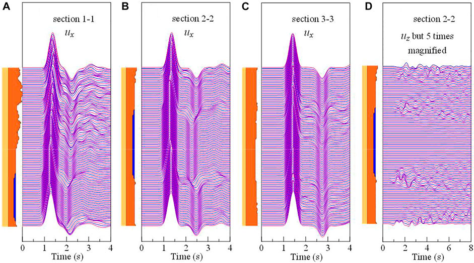
FIGURE 14. (A) Displacement waveforms in x-direction of section 1-1; (B) Displacement waveforms in x-direction of section 2-2; (C) Displacement waveforms in x-direction of section 3-3; (D) Displacement waveforms in z-direction of section 2-2.
In summary, our code can efficiently simulate marine seismoacoustic scattering in large-scale marine site.
5 Conclusion
We have developed a new FEM simulation code for efficient modeling of seismoacoustic scattering in 2D/3D large-scale marine areas. This code improves the calculation efficiency of marine seismic simulation from two aspects: calculation method and computational strategy. In terms of calculation method, different media (fluid, saturated porous medium, solid) are successfully unified into the generalized saturated porous media framework by extending Biot’s saturated porous media theory and continuous conditions between different media, which means that different media can be simulated simultaneously in a single solver. The response is obtained by the lumped mass and explicit integration scheme, which can avoid solving large system of equations, and have high computational efficiency. In terms of computational strategy, regular hexahedral elements are used to discretize the computational model, and EBE parallel computing strategy is adopted, which improves the robustness of computing and reduces the demand for computational memory. The computational efficiency and accuracy of our code was examined by a 3D horizontal layered model with the plane P-wave incidence, the applicability and the effectiveness were demonstrated by simulating seismoacoustic scattering in Tokyo Bay.
In this paper, the model is discretized into cubit elements with unified size. However, when the medium wave velocity in the model varies greatly, or the surface terrain of the model changes drastically, the element size needs to be reduced to meet the numerical stability requirements, which increases the computational load. In the subsequent study, the hybrid grid would be used to discretize the model in our code, which can ensure the computational accuracy and radically reduces the computational load (Ichimura et al., 2007).
Data availability statement
The raw data supporting the conclusion of this article will be made available by the authors, without undue reservation.
Author contributions
SJ: Writing—original draft, Write the code, Numerical calculation CS: Writing—review and editing, Supervision ZJ: Write the code CP: Data curation.
Funding
This paper was supported by the National Natural Science Foundation of China (No.51978337 No.U2039209).
Acknowledgments
The author thanks the Beijing paratera tech corp., LTD., for providing computing services, and Google Earth for providing Tokyo Bay topography.
Conflict of interest
The authors declare that the research was conducted in the absence of any commercial or financial relationships that could be construed as a potential conflict of interest.
Publisher’s note
All claims expressed in this article are solely those of the authors and do not necessarily represent those of their affiliated organizations, or those of the publisher, the editors and the reviewers. Any product that may be evaluated in this article, or claim that may be made by its manufacturer, is not guaranteed or endorsed by the publisher.
References
Bao, X., Liu, J., Chen, S., and Wang, P. (2022). Seismic analysis of the reef-seawater system: Comparison between 3D and 2D models. J. Earthq. Eng. 26 (6), 3109–3122. doi:10.1080/13632469.2020.1785976
Biot, M. A. (1962). Mechanics of deformation and acoustic propagation in porous media. J. Appl. Phys. 33 (4), 1482–1498. doi:10.1063/1.1728759
Biot, M. A. (1956). Theory of propagation of elastic waves in a fluid-saturated porous solid. I. low-frequency range. J. Acoust. Soc. Am. 28 (2), 168–178. doi:10.1121/1.1908239
Chen, S. L., Cheng, S. L., and Ke, X. F. (2019b). A unified computational framework for fluid-solid coupling in marine earthquake engineering: Irregular interface case. Chin. J. Theor. Appl. Mech. 51 (5), 1517–1529. (in Chinese with English abstract).
Chen, S. L., Ke, X. F., and Zhang, H. X. (2019a). A unified computational framework for fluid-solid coupling in marine earthquake engineering. Chin. J. Theor. Appl. Mech. 51 (2), 594–606. (in Chinese with English abstract).
Chen, S. L., and Liao, Z. P. (2003). Multi-transmitting formula for attenuating waves. Acta Seismol. Sin. 16 (3), 283–291. doi:10.1007/s11589-003-0032-7
Deresiewicz, H., and Rice, J. T. (1964a). The effect of boundaries on wave propagation in a liquid-filled porous solid: V. Transmission across a plane interface. Bull. Seismol. Soc. Am. 54 (1), 409–416. doi:10.1785/bssa0540010409
Deresiewicz, H. (1964b). The effect of boundaries on wave propagation in a liquid-filled porous solid: VII. Surface waves in a half-space in the presence of a liquid layer. Bull. Seismol. Soc. Am. 54 (1), 425–430. doi:10.1785/bssa0540010425
Drolia, M., Mohamed, M. S., Laghrouche, O., Seaid, M., and Kacimi, A. E. (2020). Explicit time integration with lumped mass matrix for enriched finite elements solution of time domain wave problems. Appl. Math. Model. 77 (2), 1273–1293. doi:10.1016/j.apm.2019.07.054
Ho-Le, K. (1988). Finite element mesh generation methods: A review and classification. Computer-Aided Des. 20 (1), 27–38. doi:10.1016/0010-4485(88)90138-8
Hu, J. J., Tan, J. Y., and Zhao, J. X. (2020). New GMPEs for the Sagami bay region in Japan for moderate magnitude events with emphasis on differences on site amplifications at the seafloor and land seismic stations of K-NET. Bull. Seismol. Soc. Am. 110 (5), 2577–2597. doi:10.1785/0120190305
Hughes, T. (2000). The finite element method: Linear static and dynamic finite element analysis. Beijing China: Prentice-Hall.
Ichimura, T., Hori, M., and Kuwamoto, H. (2007). Earthquake motion simulation with multiscale finite-element analysis on hybrid grid. Bull. Seismol. Soc. Am. 97 (4), 1133–1143. doi:10.1785/0120060175
Ke, X. F., Chen, S. L., and Zhang, H. X. (2019). Free-field analysis of seawater-seabed system for incident plane P-SV waves. J. Vib. Eng. 32 (6), 966–976. (in Chinese with English abstract).
Koketsu, K., Fujiwara, H., and Ikegami, Y. (2004). Finite-element simulation of seismic ground motion with a voxel mesh. Pure Appl. Geophys. 161 (11-12), 2463–2478. doi:10.1007/s00024-004-2557-7
Koketsu, K., Miyake, H., Afnimar, , and Tanaka, Y. (2009). A proposal for a standard procedure of modeling 3-D velocity structures and its application to the Tokyo metropolitan area, Japan. Tectonophysics 472 (1-4), 290–300. doi:10.1016/j.tecto.2008.05.037
Li, C., Hao, H., Li, H. N., Bi, K. M., and Chen, B. K. (2017). Modeling and simulation of spatially correlated ground motions at multiple onshore and offshore sites. J. Earthq. Eng. 21 (3), 359–383. doi:10.1080/13632469.2016.1172375
Link, G., Kaltenbacher, M., Breuer, M., and Döllinger, M. (2009). A 2D finite-element scheme for fluid-solid-acoustic interactions and its application to human phonation. Comput. Methods Appl. Mech. Eng. 198 (41-44), 3321–3334. doi:10.1016/j.cma.2009.06.009
Liu, J. B., Bao, X., Wang, D. Y., and Wang, P. G. (2019). Seismic response analysis of the reef-seawater system under incident SV wave. Ocean. Eng. 180, 199–210. doi:10.1016/j.oceaneng.2019.03.068
Liu, S. L., Yang, D. H., Dong, X. P., Liu, Q. C., and Zheng, Y. C. (2017). Element-by-element parallel spectral-element methods for 3-D teleseismic wave modeling. Solid earth. 8 (5), 969–986. doi:10.5194/se-8-969-2017
Lokke, A. (2019). Direct finite element method for nonlinear earthquake analysis of concrete dams including dam-water-foundation rock interaction. Berkeley: Pacific Earthquake Engineering Research Center Headquarters at the University of California.
Maeda, T., Takemura, S., and Furumura, T. (2017). OpenSWPC: An open-source integrated parallel simulation code for modeling seismic wave propagation in 3D heterogeneous viscoelastic media. Earth, Planets Space 69 (1), 102. doi:10.1186/s40623-017-0687-2
Moczo, P., Kristek, J., and Halada, L. (2000). 3D fourth-order staggered-grid finite difference schemes: Stability and grid dispersion. Bull. Seismol. Soc. Am. 90 (3), 587–603. doi:10.1785/0119990119
Morency, C., and Tromp, J. (2008). Spectral-element simulations of wave propagation in porous media. Geophys. J. Int. 175 (1), 301–345. doi:10.1111/j.1365-246x.2008.03907.x
Nakamura, T., Nakano, M., Hayashimoto, N., Takahashi, N., Takenaka, H., Okamoto, T., et al. (2014). Anomalously large seismic amplifications in the seafloor area off the Kii peninsula. Mar. Geophys. Res. 35 (3), 255–270. doi:10.1007/s11001-014-9211-2
Nakamura, T., Takenaka, H., Okamoto, T., and Kaneda, Y. (2012). FDM simulation of seismic-wave propagation for an aftershock of the 2009 Suruga bay earthquake: Effects of ocean-bottom topography and seawater layer. Bull. Seismol. Soc. Am. 102 (6), 2420–2435. doi:10.1785/0120110356
Nakamura, T., Takenaka, H., Okamoto, T., Ohori, M., and Tsuboi, S. (2015). Long-period ocean-bottom motions in the source areas of large subduction earthquakes. Sci. Rep. 5 (1), 1–10. doi:10.1038/srep16648
Oba, A., Furumura, T., and Maeda, T. (2020). Data assimilation-based early forecasting of long-period ground motions for large earthquakes along the Nankai trough. J. Geophys. Res. Solid Earth 125 (6), 1–19. doi:10.1029/2019jb019047
Okamoto, T., and Takenaka, H. (1999). A reflection/transmission matrix formulation for seismoacoustic scattering by an irregular fluid–solid interface. Geophys. J. Int. 139 (2), 531–546. doi:10.1046/j.1365-246x.1999.00959.x
Okamoto, T., Takenaka, H., Nakamura, T., and Aoki, T. (2010). Accelerating large-scale simulation of seismic wave propagation by multi-GPUs and three-dimensional domain decomposition. Earth, Planets Space 62 (12), 939–942. doi:10.5047/eps.2010.11.009
Okamoto, T., Takenaka, H., Nakamura, T., and Hara, T. (2017). FDM simulation of earthquakes off Western Kyushu, Japan, using a land-ocean unified 3D structure model. Earth, Planets Space 69 (1), 88–102. doi:10.1186/s40623-017-0672-9
Takemura, S., Kubo, H., Tonegawa, T., Saito, T., and Shiomi, K. (2019). Modeling of long-period ground motions in the nankai subduction zone: Model simulation using the accretionary prism derived from oceanfloor local S-wave velocity structures. Pure Appl. Geophys. 176 (2), 627–647. doi:10.1007/s00024-018-2013-8
Takemura, S., Okuwaki, R., Kubota, T., Shiomi, K., Kimura, T., and Noda, A. (2020). Centroid moment tensor inversions of offshore earthquakes using a three-dimensional velocity structure model: Slip distributions on the plate boundary along the nankai trough. Geophys. J. Int. 222 (2), 1109–1125. doi:10.1093/gji/ggaa238
Takemura, S., Yoshimoto, K., and Shiomi, K. (2021). Long-period ground motion simulation using centroid moment tensor inversion solutions based on the regional three-dimensional model in the Kanto Region, Japan. Earth, Planets Space 73 (1), 15. doi:10.1186/s40623-020-01348-2
Wang, X., and Zhan, Z. W. (2020). Moving from 1-D to 3-D velocity model: Automated waveform-based earthquake moment tensor inversion in the los angeles region. Geophys. J. Int. 220 (1), 218–234. doi:10.1093/gji/ggz435
Keywords: fluid-solid interaction, generalized saturated porous medium, marine seismoacoustic scattering, parallel computation, Tokyo Bay
Citation: Jirong S, Shaolin C, Jiao Z and Puxin C (2023) Unified framework based parallel FEM code for simulating marine seismoacoustic scattering. Front. Earth Sci. 10:1056485. doi: 10.3389/feart.2022.1056485
Received: 28 September 2022; Accepted: 19 December 2022;
Published: 10 January 2023.
Edited by:
Yefei Ren, Institute of Engineering Mechanics, China Earthquake Administration, ChinaReviewed by:
Andrea Montanino, University of Naples Federico II, ItalyBa Zhenning, Tianjin University, China
Copyright © 2023 Jirong, Shaolin, Jiao and Puxin. This is an open-access article distributed under the terms of the Creative Commons Attribution License (CC BY). The use, distribution or reproduction in other forums is permitted, provided the original author(s) and the copyright owner(s) are credited and that the original publication in this journal is cited, in accordance with accepted academic practice. No use, distribution or reproduction is permitted which does not comply with these terms.
*Correspondence: Chen Shaolin, aWVtY3NsQG51YWEuZWR1LmNu