Anisotropic structure of the Australian continent

The Australian continent preserves some of the oldest lithosphere on Earth in the Yilgarn, Pilbara, and Gawler Cratons. In this study we present shear wave splitting and Ps receiver function results at long running stations across the continent. We use these results to constrain the seismic anisotropic structure of Australia’s cratons and younger Phanerozoic Orogens. For shear wave splitting analysis, we utilize SKS and SKKS phases at 35 broadband stations. For Ps receiver function analysis, which we use to image horizontal boundaries in anisotropy, we utilize 14 stations. Shear wave splitting results at most stations show strong variations in both orientation of the fast direction and delay time as a function of backazimuth, an indication that multiple layers of anisotropy are present. In general, observed fast directions do not appear to be the result of plate motion alone, nor do they typically follow the strike of major tectonic/geologic features at the surface, although we do point out several possible exceptions. Our Ps receiver function results show significant variations in the amplitude and polarity of receiver functions with backazimuth at most stations across Australia. In general, our results do not show evidence for distinctive boundaries in seismic anisotropy, but instead suggest heterogenous anisotropic structure potentially related to previously imaged mid-lithospheric discontinuities. Comparison of Ps receiver function and shear wave splitting results indicates the presence of laterally variable and vertically layered anisotropy within both the thicker cratonic lithosphere to the west, as well as the Phanerozoic east. Such complex seismic anisotropy and seismic layering within the lithosphere suggests that anisotropic fabrics may be preserved for billions of years and record ancient events linked to the formation, stabilization, and evolution of cratonic lithosphere in deep time.

1 Introduction

Earth’s interior is commonly divided into layers by one of two criteria: composition or rheology. The outermost rheological layer is the lithosphere, a rigid shell that translates coherently above the flowing asthenosphere and is composed of portions of two compositional layers, the crust and the mantle. In some instances, the lithosphere is considered to be that portion of the Earth engaged in plate tectonics and is referred to as the tectosphere (Jordan, 1975). Increasing evidence suggests the lithosphere is heterogeneous in many geophysical properties: magnetotellurics (e.g., Selway, 2018; Bedrosian and Finn, 2021), tomography (e.g., Yoshizawa, 2014), attenuation (e.g., Kennett and Abdullah, 2011), reflectivity (e.g., Kennett et al., 2017), reflection (e.g., Worthington et al., 2015), refraction (Musacchio et al., 2004), shear wave splitting (e.g., Chen et al., 2018), and receiver functions (e.g., Hopper and Fischer, 2015). One of the key findings from some of these studies is that heterogeneity within the Earth’s upper mantle is often expressed as anisotropy of material properties such as seismic wavespeeds (Debayle et al., 2016), strength (Vauchez et al., 1998), and electrical conductivity (Du Frane et al., 2005). In this study, we present results at long-running stations across the entire Australian continent from two complementary techniques, shear wave splitting and receiver functions, to provide a detailed accounting of anisotropy within the Australian lithosphere—which in some instances has evolved over billions of years of geologic history. We examine cratonic Australia (regions tectonically inactive for at least one billion years) and the younger, Phanerozoic eastern margin for evidence of preserved and inherited seismic lithospheric structure. Importantly, we observe complex seismic structure not only in the cratons, but also in Phanerozoic Australia.

1.1 Shear wave splitting background

Seismic structures are often assumed to be isotropic—meaning wave speed is not directionally dependent. Yet many of the Earth’s constituent minerals have strongly anisotropic crystal forms leading to variations in speed of light or seismic wavespeeds according to the direction energy propagates. The observation of seismic anisotropy in Earth’s lithosphere and asthenosphere thus requires the bulk alignment of crystal forms within the crust and/or mantle. At crustal depths, minerals such as quartz, mica, and amphibole are seismically anisotropic (Brownlee et al., 2017). At upper mantle depths, the dominant mineral is olivine, which is strongly anisotropic, exhibiting up to 22.3% single-crystal anisotropy for S-waves (Kumazawa and Anderson, 1969). In the crust, anisotropy may be expressed as either shape-preferred orientation (alignment of fractures or magmatic bodies) or lattice-preferred orientation (alignment of mineral crystals due to strain; LPO). In the mantle, the force of plate motion or convection may create LPO, although shape-preferred orientation may also be present as melt-aligned structures, though this occurs predominantly in rift settings (e.g., Vauchez et al., 2000; Walker et al., 2004). While the mechanics behind LPO formation are complicated, in the upper mantle they can usually be simplified to a case of dislocation glide where shear in crystals mirrors shear due to plate motion, and fast directions are parallel to flow (Karato et al., 2008).

One of the most used methods to image seismic anisotropy is known as shear wave splitting. A shear wave encountering an anisotropic medium will be split into two orthogonal quasi-shear waves (one fast, one slow). As the waves propagate through the medium, they travel at different wave speeds, accruing a delay time between the two waves. Upon reaching a receiver, the delay time between the waves (the combined result of the strength of anisotropy and thickness of the layer) and the fast direction of the medium (or the alignment of mineral crystals) can be measured; see Section 2.1 for more information on this methodology. This method has been used in many different tectonic settings to measure the seismic anisotropy of crust and mantle lithosphere, including subduction zones (Long and Silver, 2008), mid-ocean ridges (Conder, 2007), and tectonically quiescent regions such as cratons (Eakin et al., 2021).

1.2 Ps receiver function background

Earth’s interior is composed of rocks with different material properties, such as velocity and density. Strong contrasts in these properties across horizontal to gently dipping layers can result in the conversion from a P-wave to an S-wave, or vice versa. These converted phases can be used with the unconverted phase to deconvolve a structural component from the signal. This is known as a receiver function, and has been used to image a number of lithologic and mineralogic boundaries within the Earth such as sediment-basement contacts (Liu et al., 2018), deep crustal mineralogical/seismic structure (Hopper et al., 2017), the crust-mantle boundary (the Moho; Reading and Kennett, 2003), the lithosphere-asthenosphere boundary (Ford et al., 2010), seismic wave speed discontinuities internal to thick lithosphere (known as mid-lithospheric discontinuities; Wirth and Long, 2014), and the mantle transition zone (Ba et al., 2020).

In this study, we present results from Ps receiver functions across Australia. This method provides excellent vertical resolution of seismic boundaries. Because the direct and converted arrivals are time separated, Ps receiver functions image the Moho well. Additionally, backazimuthal variations in the amplitude and polarity of transverse-component receiver functions can be used to detect changes in seismic anisotropy across boundaries (Levin and Park, 1997; Schulte-Pelkum and Mahan, 2014; Park and Levin, 2016). This method has been used to estimate seismic anisotropy in several settings, such as subduction zones (Wirth and Long, 2012), tectonically quiescent interiors (Wirth and Long, 2014; Ford et al., 2016; Chen et al., 2021b), and orogens (Long et al., 2017). However, Moho multiples can obscure arrivals from the uppermost mantle, making them less suitable for imaging the lithosphere-asthenosphere boundary in some instances (Bostock, 1997; Bostock, 1998). Previous continent-wide receiver function studies of Australia provide independent constraints on both the seismic structure of the lithospheric mantle and the depth of lithosphere-asthenosphere boundary, but these studies have assumed a largely isotropic mantle (Ford et al., 2010; Birkey et al., 2021). Calculation of anisotropic Ps receiver functions will improve understanding of the seismic structure and layering of the Australian continent and provide a complementary dataset to shear wave splitting.

1.3 Tectonic background

The Australian continent has a long geologic history spanning the Archean to present. It can be divided into four broad regions (Figure 1). In the western two-thirds of the continent, there are three composite cratons: the West Australian Craton, composed of the Archean Pilbara and Yilgarn Cratons as well as Proterozoic Orogens and basins; the South Australian Craton, with the Archean Gawler Craton in the center, the Proterozoic Curnamona Craton along the eastern margin, and Proterozoic basins between; and the North Australian Craton, composed of the Proterozoic Kimberly Craton in the northwest, and Proterozoic basins and orogens throughout. The North Australian Craton and West Australian Craton were joined together around 1.8 Ga, evidence of which is preserved in the Rudall Complex and Arunta Inlier (Collins and Shaw, 1995; Smithies and Bagas, 1997; Li, 2000). Between 1.3 and 1.1 Ga, the South Australian Craton completed its final docking with the West Australian Craton and North Australian Craton during the Musgrave and Albany-Fraser Orogenies (Clarke et al., 1995; Myers et al., 1996). To the east are a series of Phanerozoic orogens that were accreted to the cratonic core: the Cambrian Delamerian (Marshak and Flöttmann, 1996), the Cambrian to Late Permian Lachlan and Thomson (Murray and Kirkegaard, 1978; Foster and Gray, 2000), and the Carboniferous to Early Mesozoic New England Orogen (Coney et al., 1990). Separating the cratons and Phanerozoic orogens to the east is the Tasman Line, a boundary inferred predominantly from surface geology (Direen and Crawford, 2003).

FIGURE 1

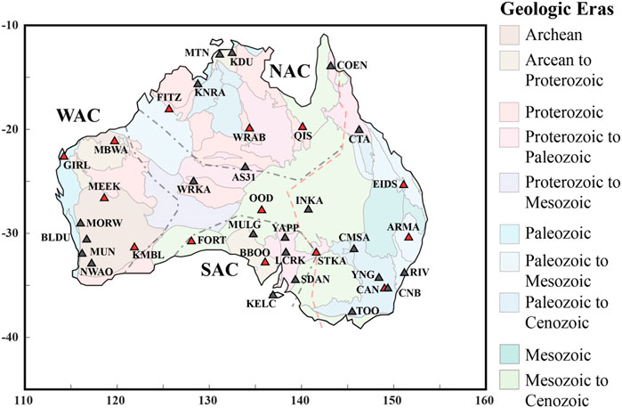
FIGURE 1. Map of stations used in this study. Red triangles indicate stations used in both shear wave splitting and receiver function analysis. Gray triangles indicates stations used only for shear wave splitting. Background shows significant geologic divisions of Australia, simplified from Fraser et al. (2007). Dashed red line shows location of the Tasman Line. Dashed gray lines mark inferred boundaries of cratonic blocks. NAC–North Australian Craton; SAC–South Australian Craton; WAC–West Australian Craton.

1.4 Previous geophysical studies relevant to this study

Previous shear wave splitting studies have indicated complex anisotropic structure of the Australian lithosphere. Continental studies have indicated frequency dependent splitting, implying depth variation in anisotropy (Clitheroe and Van der Hilst, 1998; Özalbey and Chen, 1999). A large percentage of nulls, results indicating no splitting or coming from backazimuths aligned with the fast or slow direction, have been calculated in both continental and local shear wave splitting studies (Özalbey and Chen, 1999; Heintz and Kennett, 2006; Chen et al., 2021a; Eakin et al., 2021). Several studies have indicated potential correlation between fast directions and features observed at the surface or in the crust: at station WRAB (NAC), fast direction is consistent with Proterozoic faulting (Clitheroe and Van der Hilst, 1998); splitting at KMBL in the Yilgarn Craton (WAC) roughly mirrors the trend of the Eastern Goldfields Terrane (Chen et al., 2021b); results from the BILBY network near the North Australian Craton’s Tenant Creek Inlier match its geometry (Eakin et al., 2021); and stations in eastern Australia have been shown to have fast directions that are subparallel to the structural trends of Phanerozoic fold belts or the Tasman Line—shown in Figure 1 as a dashed red line (Clitheroe and Van der Hilst, 1998; Heintz and Kennett, 2005; Bello et al., 2019). In general, fast directions across the continent due not mirror apparent plate motion, suggesting a contribution from fossilized lithospheric anisotropy (Clitheroe and Van der Hilst, 1998; Heintz and Kennett, 2005).

Tomographic studies have also examined anisotropy within the Australian lithosphere and asthenosphere. In general, azimuthal anisotropy is weaker above 150 km with complex patterns; below that, fast directions rotate to more N-S, mirroring plate motion (Debayle and Kennett, 2000; Simons et al., 2002; Debayle et al., 2005; Fishwick and Reading, 2008). While these models suggest broad trends such as shallower anisotropy roughly oriented E-W and deeper anisotropy oriented N-S, there are some variations. For instance, Fishwick and Reading (2008) find weak anisotropy within the center of Australia at 75 km, with stronger anisotropy around the edges; while most fast directions are oriented N-S by 250 km, their model suggests complex anisotropy within the WAC and SAC. Simons et al. (2002) constrain complex patterns that do not correlate to surface features down to at least 200 km, with a rotation to more N-S-oriented patterns by 300 km depth. Studies of radial anisotropy have also suggested multilayered anisotropy, with complex changes through the lithosphere and into the asthenosphere (Debayle and Kennett, 2000; Yoshizawa and Kennett, 2015). As with azimuthal anisotropy, radial anisotropy is laterally heterogeneous throughout the continent. The strongest radial anisotropy is observed in Proterozoic suture zones of central Australia, with somewhat weaker radial anisotropy in the NAC and WAC (Yoshizawa and Kennett, 2015).

Anisotropic receiver function analysis of Australia has thus far been relatively limited. Chen et al. (2021b) calculated Ps receiver functions in the Yilgarn Craton and found evidence for multiple layers of anisotropy. Ford et al. (2010) and Birkey et al. (2021) utilized Sp receiver functions to characterize discontinuity structure of the lithospheric mantle—while these analyses did not constrain anisotropy, they found evidence for mid-lithospheric discontinuities within cratonic Australia, which some have argued may be due to anisotropic layering (Rychert and Shearer, 2009; Wirth and Long, 2014).

2 Materials and methods

We used 35 stations for shear wave splitting, including those from the Australian National Seismograph Network (AU, 32 stations; DOI https://dx.doi.org/10.26186/144675), the Global Seismograph Network (IU and II; DOI https://doi.org/10.7914/SN/IU and https://doi.org/10.7914/SN/II), and the French Global Network of Seismological Broadband Stations (G, one station; DOI http://doi.org/10.18715/GEOSCOPE.G). Ps receiver functions used 14 total stations from the same networks: 11 from the AU network, and one each from the IU, II, and G networks. Data used in this study were accessed using the IRIS Data Management Center. They are free and publicly available.

2.1 Shear wave splitting

We used core-refracted phases (i.e., SKS and SKKS) to calculate our shear wave splitting results. These have the benefit of a “reset” due to conversion from P-to-S at the core-mantle boundary; thus, the anisotropy observed at the surface is only due to receiver-side effects (assumed to be dominantly in the upper mantle, though this may not be the case). Phases were limited to 85°–130° epicentral distance to avoid phase contamination, to events M_w 5.5 and greater to maximize the signal-to-noise ratio, and no event depth limits were applied. Signals were filtered at multiple frequency bands between 0.01 and 1.0 Hz to maximize the signal-to-noise ratio. Additionally, changes in splitting parameters with frequency bands have been linked to changes in anisotropy with depth (i.e., higher frequencies are linked to shallower depths and lower frequencies to greater depths; Eakin and Long, 2013), though we do not observe any obvious frequency dependence.

Splits were calculated in an updated version of Splitlab (Wüstefeld et al., 2008; Deng et al., 2017), a free, publicly available MATLAB plugin. All splitting results in this paper are from the rotation correlation method (Bowman and Ando, 1987): this method takes the signal on both components, rotates them in 1° increments, and time shifts them in 0.1 s increments. For each rotation and each time shift, correlation between the signals is calculated. The pair with the maximum correlation represents the fast direction and delay time of the split. One limitation of this method is a systematic misorientation of 45° at near-null directions; this can be accounted for with modeling of the splitting parameters, detailed in Section 3.3 (Wüstefeld and Bokelmann, 2007; Eakin et al., 2019). To check for the quality of splits, we also calculate splitting parameters using the minimum energy and eigenvalue methods (Silver and Chan, 1991). Fast directions between methods within 25° of one another and delay times within 0.4 s are required for fair and null splits, but not poor splits; we show an example split and null in Supplementary Figures S1, 2. Finally, splitting intensity is calculated to check whether the split is a null—a splitting intensity value close to 0 indicates a null value, and in cratons the absolute value tends to be smaller than in other regions. The signal-to-noise ratio was required to be above 5.0. Finally, the shape of the particle motion before and after correction for the preferred fast direction and delay time was examined: before correction particle motion should be elliptical, then rectilinear after correction. We check station orientation using the Latest Assessment of Seismic Station Observations (LASSO).

2.2 Ps receiver functions

Events for Ps receiver function analysis were epicentrally limited to 30°–95° with no depth limit. Stations with more than 5 years of data had a higher magnitude cutoff of 5.8 to maximize the signal-to-noise ratio, while stations with less than 5 years of data had a lower magnitude cutoff of 5.6 to maximize the number of waveforms available. Preprocessing of receiver functions included: cutting traces to identical length; detrending and demeaning waveforms; bandpass filtering from 0.02 to 2.0 Hz; visually sorting waveforms with clear P-wave arrivals; and manually picking P-wave arrivals in the Seismic Analysis Code (SAC). Waveforms were rotated into vertical, radial, and transverse components (with most Ps energy occurring on the radial component). Receiver functions were calculated with a 65 s data window. All backazimuths were calculated in 10° bins with a minimum of two events required per bin. Deconvolution of the daughter phase (Ps wave) was performed in the frequency domain using the multiple-taper spectral correlation method (Park and Levin, 2016). Once deconvolution was performed, receiver functions were migrated from time to depth using the local tomography model AuSREM (Kennett and Salmon, 2012; Kennett et al., 2013; Salmon et al., 2013). We report receiver functions at 0.75 Hz—this frequency provides more clearly separated pulses than 0.5 Hz without introducing higher frequency noise (such as seen at 1.0 or 2.0 Hz).

3 Results

Below we present results first for shear wave splitting, then receiver functions. We describe shear wave splitting results in terms of station-averaged splitting parameters (Section 3.1), then according to backazimuthal variations in said parameters (Section 3.2), and finally in terms of single-layer modeling (Section 3.3). We then describe receiver functions in terms of crustal and Moho structure, followed by mantle structure (Section 3.4).

3.1 Station averaged splitting parameters

A total of 522 non-null splits were calculated. Null results (i.e., non-splitting) are evidence of no anisotropy, weak anisotropy, or alignment of the backazimuth of the incoming wave with a fast or slow direction (Savage, 1999). There was a total of 409 nulls detected. Events for both splits and nulls are clustered around four backazimuths: 30° (199 results), 150° (206 results), 190° (189 results), and 300° (91 results). These correspond to the subduction zone along the northern Pacific plate, the subduction zone along the west coast of South America, the spreading center between the Antarctic and South American plates, and the Himalayan collision zone, respectively (Figure 2).

FIGURE 2

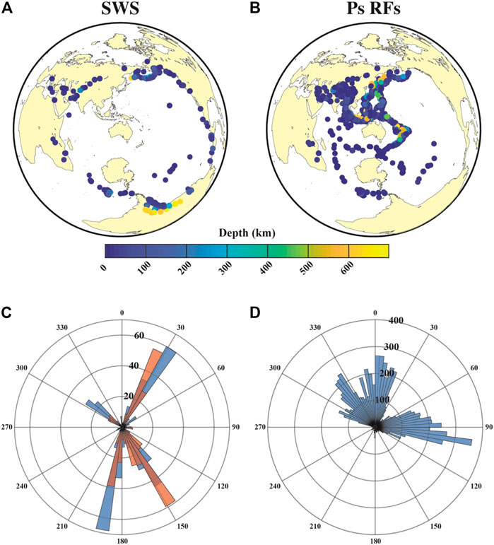
FIGURE 2. Event information for both methods used in this study. (A) Map of events used for shear wave splitting, color coded according to event depth. (B) Map of events used for receiver functions, color coded according to event depth. (C) Polar histogram of event distribution by backazimuth for shear wave splitting. Blue bins are splitting results, while orange bins are null results. (D) Polar histogram of event distribution by backazimuth for receiver functions.

Shear wave splitting results are often presented as station averages. In Figure 3 we display an arithmetic mean for the average fast direction and delay time at each station, plotted on top of tectonic terranes. Average fast directions at all stations trend either N-S or NE-SW, and there are few correlations between tectonic terranes inferred at the surface and average fast directions; however, there are slight variations between regions (Supplementary Figures S3). Delay times among all regions tend to be around 0.6 s (Supplementary Figures S4), smaller than the average at stations globally but consistent with previous results in Australia (e.g., Heintz and Kennett, 2005).

FIGURE 3

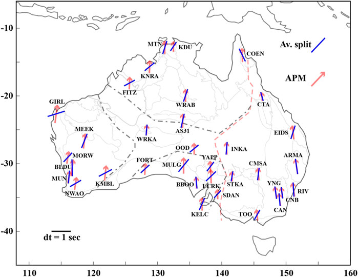
FIGURE 3. Average shear wave splitting parameters plotted against apparent plate motion from the HS3-NUVEL 1A model (Gripp and Gordon, 2002). An example split with a fast direction of 90° and a delay time of 1 s is shown in the lower left.

In the same figure, we also plot average fast directions against plate motion from a hotspot frame of reference using HS3-NUVEL 1A (Gripp and Gordon, 2002). At 25 of the stations analyzed, fast direction and plate motion disagree by more than 10°. One station (MBWA) has only nulls and is therefore not included in this discussion. The remaining nine stations with a fast direction within 10° of absolute plate motion are ARMA, BBOO CAN, CNB, INKA, MULG, RIV, WRKA, and YNG. Agreement between fast direction and plate motion is often assumed to be the case in tectonically quiescent regions, based on both splitting observations (e.g., Vinnik et al., 1992) and laboratory studies of olivine crystals (Karato et al., 2008). Stations ARMA, CAN, CNB, RIV, and YNG are along the eastern margin of the continent where the lithosphere is younger and thinner, and thus splitting directions may be more heavily influenced by plate motion. While station INKA is on somewhat thicker lithosphere than those ot its east, it is to the east of the Tasman Line—generally recognized as the transition between cratonic and Phanerozoic Australia. Fast directions at station WRKA are clustered near -60° (7 splits) and 60° (8 splits), so the averaging of these two bins results in a near-zero fast direction. Stations BBOO and MULG have clusters of fast directions ∼140° apart (near -70° and 70°), again resulting in a fast direction closer to zero. While nine stations have average fast directions in good agreement with plate motion, the averaging of splitting parameters smooths out significant backazimuthal variations seen in the results (see Section 3.2). Therefore, the anisotropic fabric inferred from splitting is not likely to be controlled solely by plate motion even at those stations where there is good agreement between average splitting direction and absolute plate motion. We also note that Additionally, the rotation correlation method can produce systematic 45° misorientations from the true fast direction (Wüstefeld and Bokelmann, 2007; Eakin et al., 2019), which will lead to inaccurate station averages: to address this possibility, we model results by station in Section 3.3.

3.2 Backazimuthal variation in splitting

Layered anisotropy should produce backazimuthal variations in fast direction and delay time. As seen in Figure 4, we observed this in Australia. In general, stations with longer deployment times have more data and more backazimuthal variation in splitting parameters (e.g., stations AS31 and CAN). However, clear variations in backazimuth can be seen at most stations in our study. Below, we examine the results of each region in the context of backazimuthal variations. While results are grouped by region, the varied tectonic histories of each region implies they need not be consistent. We display regional information on splitting in Table 1.

FIGURE 4

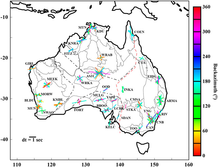
FIGURE 4. Splitting parameters color-coded by backazimuth of the event. An example split with a fast direction of 90° and a delay time of 1 s is shown in the lower left. Note that 0° and 360° are the same backazimuths.

TABLE 1

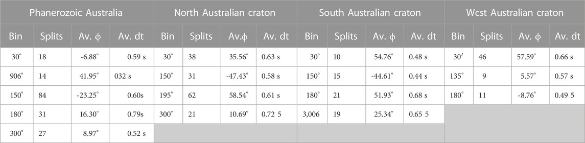
TABLE 1. Bins with the most splits for each of the four regions. The number of splits, average fast direction ?), and average delay time (dt) per bin are shown.

3.2.1 Splitting in phanerozoic Australia

This region contains the most stations (12) and the most non-null splits (190). Absolute plate motion varies somewhat from north to south and from east to west, but in general the Australian plate is moving to the north. Results are shown in Supplementary Figures S5. For each region we calculate the average absolute plate motion among stations; in Phanerozoic Australia, the average absolute plate motion is oriented at -6.40°. While splitting parameters vary significantly by backazimuth, at a given backazimuth there is some consistency in results across stations. We identified the five backazimuths in this region with the most splits: 30°, 90°, 150°, 180°, and 300°. For each of these, we found splits within ±10°, then averaged the fast direction and delay time for each subset of results. At 30° we find 18 splits, with an average fast direction of -6.88° and an average delay time of 0.59 s; this is very close to the direction of absolute plate motion. There are 14 splits in the bin centered around 90°, with an average fast direction of 41.95° and an average delay time of 0.72 s; for these splits, the average fast direction and average absolute plate motion vary by 48.35°. The 150° bin has the most splits (84), and an average fast direction of -23.25° (16.85° different from the average absolute plate motion) with an average delay time of 0.6 s. With 31 splits, the 180° bin has an average fast direction of 16.30° and average delay time of 0.79 s; the average fast direction in this bin vary from average absolute plate motion by 22.7°. Finally, the bin centered at 300° has 27 splits, an average fast direction of 8.97°, and an average delay time of 0.52 s. This last bin has a 15.37° difference between fast direction and plate motion.

In Supplementary Figures S6, we display splits for all stations according to backazimuth and inclination angle. We display splits by backazimuth against fast direction and delay time in Supplementary Figures S7, 8. While average fast directions for Phanerozoic Australia generally mirror absolute plate motion, there is still some change with backazimuth. Notably, at most stations there is a clear NE-SW fast direction orientation at both 0° and 180° backazimuth. Station ARMA has the most splits in this region, with consistency in fast direction at most backazimuths: most splits are oriented close to N-S, except for a handful near ∼160° which are oriented closer to E-W. Station EIDS has more complexity in splitting, with most splits oriented NE-SW, but some oriented N-S; there is no consistency in orientation by backazimuth. Finally, station COEN has a deviation from the general trend of stations in this region, with fast directions at 180° backazimuth oriented NW-SE.

3.2.2 Splitting in the North Australian Craton

In the North Australian Craton, the average absolute plate motion is oriented at 1.17°, a slight eastward shift from the average of Phanerozoic Australia. As with splits in Phanerozoic Australia, there is significant backazimuthal complexity in the North Australian Craton, with stations AS31 and MTN having the most splits and the most variability in fast directions and delay times (Supplementary Figures S9). Within this region there are eight stations and 180 splits. Four backazimuths were identified with the most splits (30°, 150°, 195°, and 300°): as with Phanerozoic Australia, we found splits within ±10° of these and averaged fast directions and delay times. For the first bin (30° ± 10°) there are 38 splits, an average fast direction of 35.56°, and an average delay time of 0.63 s; the average fast direction and average absolute plate motion has a large disagreement here of 34.39°. At 150° we found 31 splits, with an average fast direction of -47.43 and an average delay time of 0.58 s; this bin too has a significant disagreement between average fast direction and average absolute plate motion (48.60°). The bin centered at 195° has the most splits (62); the average fast direction is 58.54° (57.37° off from average absolute plate motion) with an average delay time of 0.61 s. Our final bin (300°) has the least splits (21), an average fast direction of 10.69 and an average delay time of 0.72 s; this bin has the smallest difference between absolute plate motion and average fast direction at 9.52°. In general, splits in the North Australian Craton do not agree with plate motion and vary significantly as a function of back azimuth.

Other than a general disagreement between absolute plate motion and station-averaged fast directions, there are no noticeable key trends across the North Australian Craton. We show variations in splitting according to backazimuth and inclination angle at each station in Supplementary Figure S10, and according to backazimuth and fast direction/delay time in Supplementary Figures S11, 12. Rather, most stations in this region exhibit considerable complexity in splitting parameters as a function of backazimuth. For instance, station AS31 has significant variability with backazimuth: splits coming from just west of 180° backazimuth are oriented NE-SW, while those coming from just east of 180° backazimuth are oriented NW-SE; for splits coming from backazimuths less than 90° or greater than 270°, the fast direction is oriented close to E-W. Station WRKA has similar behavior as31 for backazimuths close to 180°. At station WRAB, results are particularly complex and backazimuthally limited. Most splits come from close to 30°, with two dominant orientations: E-W and N-S. However, splits with a steeper incidence angle have the more N-S orientation. Station MTN is the least complex station in this region, with most splits oriented either N-S or NE-SW.

3.2.3 Splitting in the South Australian Craton

In the South Australian Craton, there are eight stations and compared to other areas in our study this region contained the fewest number of splits (72). Average absolute plate motion in the South Australian Craton is oriented at -0.82°. Four backazimuthal bins were identified: 30°, 150°, 180°, and 300°. Again, splits within ​​ ±10° of these backazimuths were identified, and an average fast direction and delay time was calculated. Regional backazimuthal splits can be seen in Supplementary Figures S13. At 30°, there are 10 splits, an average fast direction of 54.76° and 0.48 s; the fast direction and absolute plate motion are 55.58° apart. The 150° bin has 15 splits, with an average fast direction of -44.51° (43.69° different from the average absolute plate motion) and an average delay time of 0.44 s. For the 180° bin, there are 21 splits; these have an average fast direction of 51.93° and an averaged delay time of 0.68 s. In this bin, the average fast direction and the average absolute plate motion are 52.75° different. Finally, at the 300° bin, there are 19 splits, an average fast direction of 25.34°, and a delay time of 0.65 s; this last bin has a difference of 26.16° between the average fast direction and absolute plate motion. While fast direction is variable at all backazimuths, those less than 180° have delay times roughly 0.2 s smaller than those greater than 180°.

As seen in Supplementary Figures S14 and Supplementary Figures S15, 16, the most obvious trend in this region is a fast direction that is oriented NE-SW for splits coming from backazimuths just west of 180°. Station BBOO has the most complexity of fast directions in the South Australian Craton, ranging from E-W at ∼315°, to NE-SW just west of 180°, and multiple fast directions just east of 180°. Station LCRK has the most consistency, with low delay times and fast directions oriented either NE-SW or E-W.

3.2.4 Splitting in the West Australian Craton

In the West Australian Craton, there are eight stations and 78 splits. Events are more backazimuthally limited here than elsewhere, and we identified only three backazimuths with more than 10 splits (30°, 135°, and 180°). As with all other regions, splits within ±10° of each backazimuth were found and splitting parameters were averaged. See Supplementary Figures S17 for results. The average absolute plate motion is 8.05°, the most eastward orientation for any of the regions. The bin centered at 30° has 46 splits; the average fast direction is 57.59° (49.54° off from the average absolute plate motion) and the average delay time is 0.66 s. At 135°, there are nine splits, with an average fast direction of 5.57° and an average delay time of 0.57 s; this bin has a small misfit from the average absolute plate motion at 2.48°. Our last bin has 11 splits, an average fast direction of -8.76° and an average delay time of 0.49 s. The difference between average fast direction and average absolute plate motion is 16.18° in this bin.

Several broad trends are observed across multiple stations in the West Australian Craton, displayed in Supplementary Figure S18 and Supplementary Figures S19, 20. For instance, at ∼30° backazimuth, fast directions at most stations are oriented ENE-WSW (with an exception at MUN, where several splits are oriented more N-S); at 180° backazimuth there is much less consistency in fast direction between stations. At station KMBL, there is a rotation in fast direction from NE-SW close to 0° backazimuth to more E-W moving toward 90° backazimuth, then back to NE-SW at 180°. Station MEEK has a similar orientation for backazimuths just east of 0° but has a rotation to NW-SE orientations just east of 180° backazimuths. Station MUN has significant complexity, with fast direction and delay time varying even for close backazimuths.

3.3 Shear wave splitting modelling

Interpreting shear wave splitting results from the rotation correlation method is complicated by a known 45° misorientation from the true fast direction at near-null backazimuths that produces a sawtooth pattern, and a sinusoidal trend for delay times (e.g., Wüstefeld and Bokelmann, 2007). Eakin et al. (2019) empirically derived the following equations to estimate the true fast direction and delay time:

${\Phi }_{app}={\Phi }_{true}-\frac{90}{\pi }{\tan }^{-1}\cot \left(\frac{\pi }{90}\left(\psi -{\Phi }_{true}\right)\right)(1)$

${\delta }_{app}={\delta }_{true}*\left|\sin \left(\frac{\pi }{90}\left(\psi -{\Phi }_{true}\right)\right)\right|(2)$

Where Φ is fast direction, ψ is backazimuth, and δt is delay time. Using these equations, we perform a grid search over fast directions ranging from 0° to 180° in 1° increments and delay times ranging from 0.1 s to 4.0 s in 0.1 s increments. We then sum the misfits—the smallest summed misfit is the preferred true fast direction or delay time.

At some stations, this correction accounts for variability in splitting with backazimuth, but at others there is backazimuthal variability that cannot be explained through simple modeling alone. This approach is also better at finding the true fast direction or delay time than a simple averaging scheme, as fast directions that are close to 180° may counteract one another. In Table 2 we show the modeled fast direction and delay time for all stations with more than two non-null splits, as well as the summed misfit values for those models. Supplementary Figures S21 shows the modelling results for all stations included in this analysis.

TABLE 2

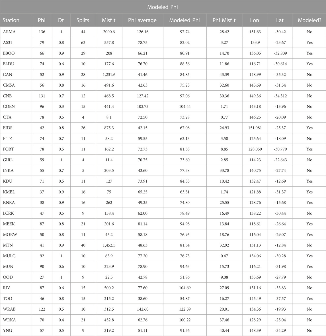
TABLE 2. Shear wave splitting modeling information.

To quantify which stations have results that are modeled by a single layer of anisotropy with misorientation from the rotation correlation method, we rely on three main criteria. First, there should be more than 10 splits at the station; while we modeled all stations with more than two splits, stations with fewer than 10 generally lack sufficient backazimuthal coverage to determine whether a model fits the data well. Second, the summed misfit between the model and results should be less than 1,000. Third, the difference between the average calculated from the sawtooth function at the same backazimuths as splits and the average of the splits themselves should be less than 25. In addition, we examine the backazimuthal coverage for all stations: some stations with sufficient data and small misfits are backazimuthally limited and thus have insufficient coverage to constrain a single correct model (such as WRAB). In total, we modeled sawtooth functions for 29 stations: 13 (45%) of these were well fit, while 16 (55%) were not. Both well-modeled and unmodeled stations are geographically distributed. Stations with a larger number of splits tend to not be well modeled, though this is not always the case (as at AS31, which has the most splits and is well modeled). We plot all modeled splitting parameters with APM in Figure 5, and the modeled and average splitting parameters in Figure 6. Unlike average fast directions, modeled fast directions do not agree with APM.

FIGURE 5

FIGURE 5. Modeled shear wave splitting parameters against apparent plate motion from the HS3-NUVEL 1A model (Gripp and Gordon, 2002). An example split with a fast direction of 90° and a delay time of 1 s is shown in the upper right.

FIGURE 6

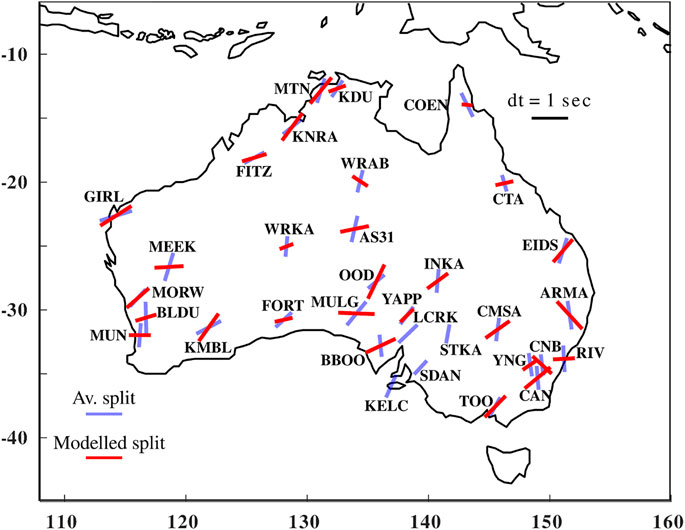
FIGURE 6. Average shear wave splitting parameters against modeled splitting parameters. An example split with a fast direction of 90° and a delay time of 1 s is shown in the upper right.

3.4 Ps receiver functions

For Ps receiver functions, 8,607 waveforms were used, averaging 615 waveforms per station. Station CAN used the most waveforms (1,135) while station OOD used the fewest (308). The small number of events at station OOD is unsurprising: using the IRIS Modular Utility for STAtisical kNowledge Gathering system (MUSTANG), probability density functions for seismic noise at the station indicate a large amount of noise above the Peterson New High Noise Model (Peterson, 1993). While station CAN is similarly noisy, it has been deployed since 1987 ensuring that there is a much longer period in which to find suitable events of high quality. Events for Ps come primarily from backazimuths between 300° and 120°. In this range there are several plate boundaries, including those of the Australian plate, those along the western Pacific plate, and the complex boundary between the Indian, Eurasian, and Australian plates (Figure 2).

We present Ps receiver function results for nine stations across the Australian continent (Figures 7–10). For the remaining stations the receiver functions are of poor quality or have issues with data availability. For instance, at stations FORT and GIRL we observe large amplitude, ringy phases with frequent polarity flips, consistent with basinal reverberations (Zelt and Ellis, 1989); Ford et al. (2010) also observed shallow crustal reverberations that prevented them from interpreting upper mantle structure at station FORT. Receiver functions were binned by backazimuth, and both the radial (corresponding to SV energy) and the transverse (corresponding to SH energy) component receiver functions were calculated. Energy on the transverse component has been shown to be primarily due to the presence of isotropic dipping structures or anisotropic boundaries (Levin and Park, 1997; Park and Levin, 2016). In the remaining results sections, we begin by first describing results associated with the crust and Moho, and then describe observed structure of the mantle. We include boundaries that are inferred to be either isotropic, anisotropic or both.

FIGURE 7

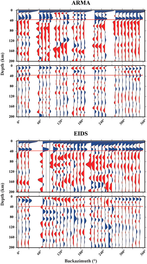
FIGURE 7. Backazimuthally-binned Ps receiver functions from Phanerozoic Australia. Top panel for each is the radial component, bottom panel is the transverse component. Blue pulses indicate a velocity increase with depth; red pulses indicate a velocity decrease with depth. The red line shows the predicted Moho depth for the station-averaged receiver functions. Backazimuth is shown on the x-axis, while depth from surface is shown on the y-axis.

FIGURE 8

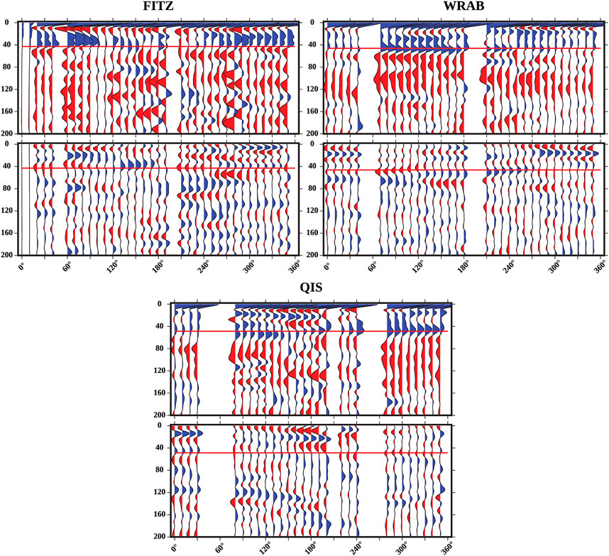
FIGURE 8. Backazimuthally-binned Ps receiver functions from the North Australian Craton (NAC). Cyan lines indicate depth of potential polarity flips, as mentioned in the text. All other features the same as in Figure 7.

FIGURE 9

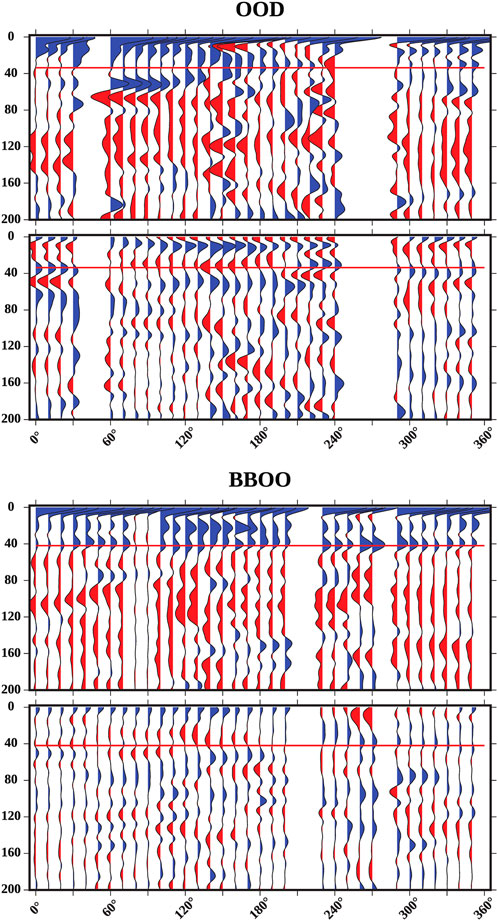
FIGURE 9. Backazimuthally-binned Ps receiver functions from the South Australian Craton (SAC). Features the same as in Figure 7.

FIGURE 10

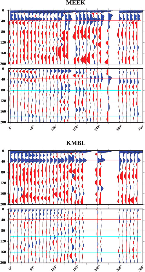
FIGURE 10. Backazimuthally-binned Ps receiver functions from the West Australian Craton (WAC). Cyan lines indicate depths of potential polarity flips, as mentioned in the text. All other features the same as in Figure 7.

3.4.1 Crust and Moho structure

The depth of the Moho is commonly mapped using Ps receiver functions, which we report below. We compare these results to those reported in the AuSREM (Kennett et al., 2017) and those calculated by Birkey et al. (2021), who used an automated receiver function method for both Sp and Ps receiver functions. With Ps receiver functions, the Moho can be identified by its positive polarity (indicating a velocity increase with depth, which is expected moving from the crust to the mantle) on radial component receiver functions. We identify Moho depths using single-station stacked radial-component receiver functions, assuming the Moho is represented by the maximum amplitude positive pulse below the direct arrival located at or near zero at each station. At stations ARMA, BBOO, EIDS, KMBL, MEEK, and WRAB, all three studies estimate similar Moho depths (within 10 km). At two stations (FITZ and OOD), our single-station stacks do not have a clear positive pulse we can associate with the Moho. At station QIS, our estimated Moho depth is within 5 km of the AuSREM estimate, but Birkey et al. (2021) did not include station QIS in their analysis. Previous global observations have indicated that older continents tend to have thicker than average crust (Laske et al., 2013): this is generally confirmed by our receiver functions. There are some exceptions: we estimate the depth of the Moho to be 32 km at station MEEK and 35 km at station KMBL, despite both being within the West Australian Craton—though previous results do potentially indicate a thicker Moho (e.g., Kennett et al., 2012; Birkey et al., 2021). Phanerozoic Australia has a crustal thickness of less than 40 km (30 km at station ARMA and 31 km at station EIDS); the North Australian Craton has the thickest crust of any region in our results, with all stations having a thickness greater than 40 km; all stations within the West Australian Craton have a crustal thickness less than 40 km.

In Phanerozoic Australia, we report results for two stations: ARMA and EIDS (seen in Figure 7). At station ARMA, the positive pulse associated with the velocity increase across the Moho on the radial component is not consistent across all backazimuths, but rather is variable in shape and amplitude, and is observed over a range of depths, between 30 and 40 km, which may be due to a laterally complex Moho. There is some positive and negative energy above the Moho, but most of the negative pulses at around 10 km depth (i.e., immediately below the direct arrival) are likely sidelobes given their timing and low amplitudes. Station EIDS has a slightly more consistent Moho pulse across backazimuths, with a clearer peak around 30 km. We observe both positive (e.g., between 160° and 190° backazimuth around 15 km) and negative energy (e.g., between 100° and 150° backazimuth around 20 km) above the Moho, potentially indicating sharp boundaries in velocity between different crustal layers.

In the North Australian Craton, we report results for three stations: FITZ, QIS, and WRAB (Figure 8). We observe the most variability in the shape and amplitude of the Moho pulse at station FITZ, with some backazimuths having no clear positive pulse associated with the transition from crust to mantle. There is a significant amount of energy above the Moho at ∼10 km, with large amplitude negative pulses between 60° and 120°, then again close to 270°: this indicates a lower-velocity layer above the Moho. Station QIS has a more consistent Moho pulse (ranging from 40 to 50 km), particularly between 280° and 350°, where the positive pulses fall roughly at the same depth (∼50 km) and have similar amplitudes. There are complex switches between positive and negative pulses above the Moho; for instance, between 120° and 190° backazimuth where a negative pulse at ∼10 km is followed by a positive pulse around 20 km, then another negative pulse ranging from 30 to 40 km depth. Station WRAB has the most consistency in the shape of its Moho pulse, with two distinct groups: one between 70° and 180° (at a depth of ∼45 km), the other between 250° and 30° (where there appear to be two or more positive pulses connected to one another without one being larger than the others). There is a large amount of positive energy above the Moho, but little negative energy except at ∼10 km where small negative pulses may represent sidelobes of the direct arrival.

For the South Australian Craton, we report Ps receiver function results for two stations: BBOO and OOD (Figure 9). Station BBOO has a relatively consistent Moho pulse at all backazimuths around 40 km, and a secondary positive pulse above the Moho around 20 km (which in some cases was the same or greater amplitude than the deeper positive pulse). There is little negative energy in the crustal portion of the receiver function. Station OOD has significantly more complex structure, with little consistency in the Moho pulse, and some backazimuths with unclear Moho arrivals. Between 150° and 170°, there are large amplitude negative pulses above the Moho at ∼10 km. There are few other negative arrivals in the sub-Moho portion of the receiver function, but positive arrivals have complex shapes and amplitudes (e.g., between 90° and 160° backazimuth where a secondary positive pulse starts immediately below the direct arrival and increases its depth with increasing backazimuth).

Finally, in the West Australian Craton we report Ps receiver function results for two stations: KMBL and MEEK (shown in Figure 10). Station KMBL has a clear, large, consistent amplitude positive pulse associated with the Moho at all backazimuths, generally around 35 km depth. There is a large amount of positive energy in the crustal portion of the receiver function (usually at ∼15 km depth), with minimal negative arrivals. The positive Moho pulse at station MEEK is also generally consistent across backazimuths (between 30 and 35 km), with some variations in pulse shape and amplitude. Like station KMBL, there is significant positive energy at most backazimuths near 15 km depth but few negative arrivals.

Overall, our results show clear Moho arrivals, possible crustal structure such as sediment-basement contacts or low-velocity zones, and some polarity flips above the Moho. As polarity flips are indicative of either dipping layers or anisotropy, this suggests the presence of one or both within the crust. However, we do not observe the two-lobe or four-lobe patterns on the transverse component receiver functions as predicted by modelling (Levin and Park, 1997; Ford et al., 2016; Park and Levin, 2016).

3.4.2 Mantle structure

As stated above, the presence of energy and polarity flips on the transverse component of receiver functions is often interpreted as being due to seismic anisotropy: our receiver functions do have significant energy below the Moho, but it is often difficult to interpret and does not follow predicted patterns of simple two-lobe or four-lobe polarity flips (e.g., Ford et al., 2016).

At station MEEK, we observe several possible polarity flips on the transverse component: first at roughly 80 km depth, then at 120 km depth, and finally at 180 km depth. Birkey et al. (2021) found two significant negative phases at station MEEK using Sp receiver functions: one at 80 km (interpreted to be a mid-lithospheric discontinuity) and one at 129 km (interpreted to be the lithosphere-asthenosphere boundary). All the Ps polarity flips appear to occur over 10s of kilometers. At station KMBL there are several gaps in backazimuthal coverage: between 200° and 240° and between 250° and 300°. These gaps make observations of polarity flips more difficult, but there do appear to be flips at 80 km, 100 km, and 160 km. As with station MEEK, these are very gradual, with pulses that extend over 10s of kilometers in depth. Previous studies reported negative phases at 79 km and 113 km, both interpreted to be mid-lithospheric discontinuities (Birkey et al., 2021). Station WRAB has polarity flips at 60 km, 100 km, 140 km, and 180 km. Mid-lithospheric discontinuities were reported at 71, 91, 135, and 198 km (Birkey et al., 2021). We display receiver functions as rose diagrams for all nine stations in Figure 11, ranging from 0 to 200 km depth. Significant complexity is present at most stations.

FIGURE 11

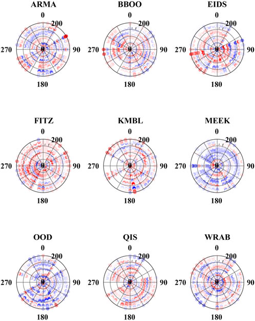
FIGURE 11. Rose diagrams of transverse-component Ps receiver functions, showing backazimuth along the circumference of circles and the depth of the phase increasing from zero at the center to 200 km at the edge. Each dot is color-coded according to the amplitude of the receiver function (blue indicates a positive phase, while red indicates a negative phase).

Our receiver functions indicate complex structure within the Australian lithosphere, as we see significant energy on transverse components with some polarity flips. However, our observed polarity flips are generally not consistent with predicted two-lobe or four-lobe patterns that a sharp boundary in seismic anisotropy would create (e.g., Levin and Park, 1997; Ford et al., 2016; Park and Levin, 2016). Due to the complexity of our results, we cannot easily generate comparative forward models, which would be necessary to infer orientations of seismic anisotropic layering in the mantle. Importantly, we note that we observe polarity flips at several stations (MEEK, KMBL, and WRAB) roughly corresponding to the same depths where Birkey et al. (2021) observed statistically significant negative phases on Sp receiver functions. Correspondence between both sets of receiver functions may indicate that MLDs at least partially arise from the presence of anisotropy at depth. Therefore, the summarizing result of our Ps receiver function analysis is that while anisotropic layering is present, it cannot provide us with unique insight into the orientation of such structures within the Australian lithosphere.

4 Discussion

For clarity, we begin our discussion with a summary of results. Station-averaged shear wave splitting fast direction mostly trend N-S, which is not generally correlated with surface features but does agree well with plate motion (though this is likely due to averaging of disparate results, not anisotropy dominated by shear at the base of the plate). Average delay times for stations across the continent are close to 0.6 s. Individual splits show a clear variation in fast direction and delay time with backazimuth in all regions, which is often seen as diagnostic of complex anisotropy. We also test whether these variations with backazimuth are due to systematic misorientation from the rotation correlation method: this seems to be the case for 13 out of 29 modelled stations. Ps receiver functions show evidence for possible crustal layering and anisotropy (as indicated by polarity flips on the transverse component); they additionally have significant energy at mantle depths with potential polarity flips, though these do not perfectly follow predicted two- or four-lobed patterns. Finally, some of these polarity flips occur at the same depths as mid-lithospheric discontinuities reported in Birkey et al. (2021).

4.1 Comparison of our results to previous shear wave splitting studies

There have been numerous previous studies that have examined the structure of the Australian continent in terms of seismic properties, including anisotropy, and other geophysical constraints (e.g., Debayle and Kennett, 2000; Heintz and Kennett, 2005; Fishwick and Reading, 2008; Ford et al., 2010; Saygin and Kennett, 2012; Wang et al., 2014; Yoshizawa and Kennett, 2015; Tesauro et al., 2020). Seismic anisotropic studies have included continental and regional shear wave splitting analysis (Clitheroe and Van der Hilst, 1998; Özalbey and Chen, 1999; Heintz and Kennett, 2005; Heintz and Kennett, 2006; Bello et al., 2019; Chen et al., 2021a; Eakin et al., 2021), and continental tomographic studies (Debayle, 1999; Debayle and Kennett, 2000; Simons et al., 2002; Debayle et al., 2005; Fishwick and Reading, 2008; Yoshizawa and Kennett, 2015). In this section we primarily focus on comparing our results to other shear wave splitting studies. In Section 4.2. we focus on comparing our shear wave splitting results to constraints from tomography and in Section 4.3. we focus on comparing our receiver function results to relevant studies. Individual and averaged splits are compared to previously published splits in Supplementary Figures S22, 23.

Eakin et al. (2021) examined shear wave splitting through central Australia, including three permanent stations that were also used in this study (stations AS31, MULG, and WRAB). That study found a significant number of null events (consistent with other studies of the Australian continent), average fast directions that paralleled topography, gravity, and magnetic trends with a transition from the Proterozoic orogens in central Australia into the North Australian Craton. They argue that their results indicate fossilized seismic anisotropy within the lithosphere, rather than from the asthenosphere (i.e., plate motion shear). While our average splits from vary significantly from those reported in Eakin et al. (2021), fast directions that were modeled to account for misorientation due to the rotation correlation method are in better agreement. However, their results are reported from the minimum energy method and included PKS phases as well, which may help to explain the discrepancies. They report an average fast direction of 72° at AS31, while our modeled fast direction was 79°. At station MULG; Eakin et al. (2021) found an average fast direction of 75°—our modeled fast direction was 92°, with five splits within 10° of their average. For station WRAB, we report a modeled fast direction of -58°, and seven splits within 10° of the -17° reported by Eakin et al. (2021). While ray paths for PKS and SK(K)S phases are nearly identical in the upper mantle, different epicentral distance ranges are used for each phase to prevent phase contamination: this may result in differences in splitting parameters, especially if there are lower mantle contributions (see Section 4.2). Additionally, very few of the events analyzed were the same between Eakin et al. (2021) and this study. However, we did identify some events in common: six at station AS31, two at station MULG, and two at station WRAB (compared in Table 3). We compare their reported minimum energy splits to our rotation correlation splits and the values we obtained from the minimum energy method. Of the 10 splits in common, seven have comparable values (four at AS31, one at station MULG, and two at station WRAB).

TABLE 3

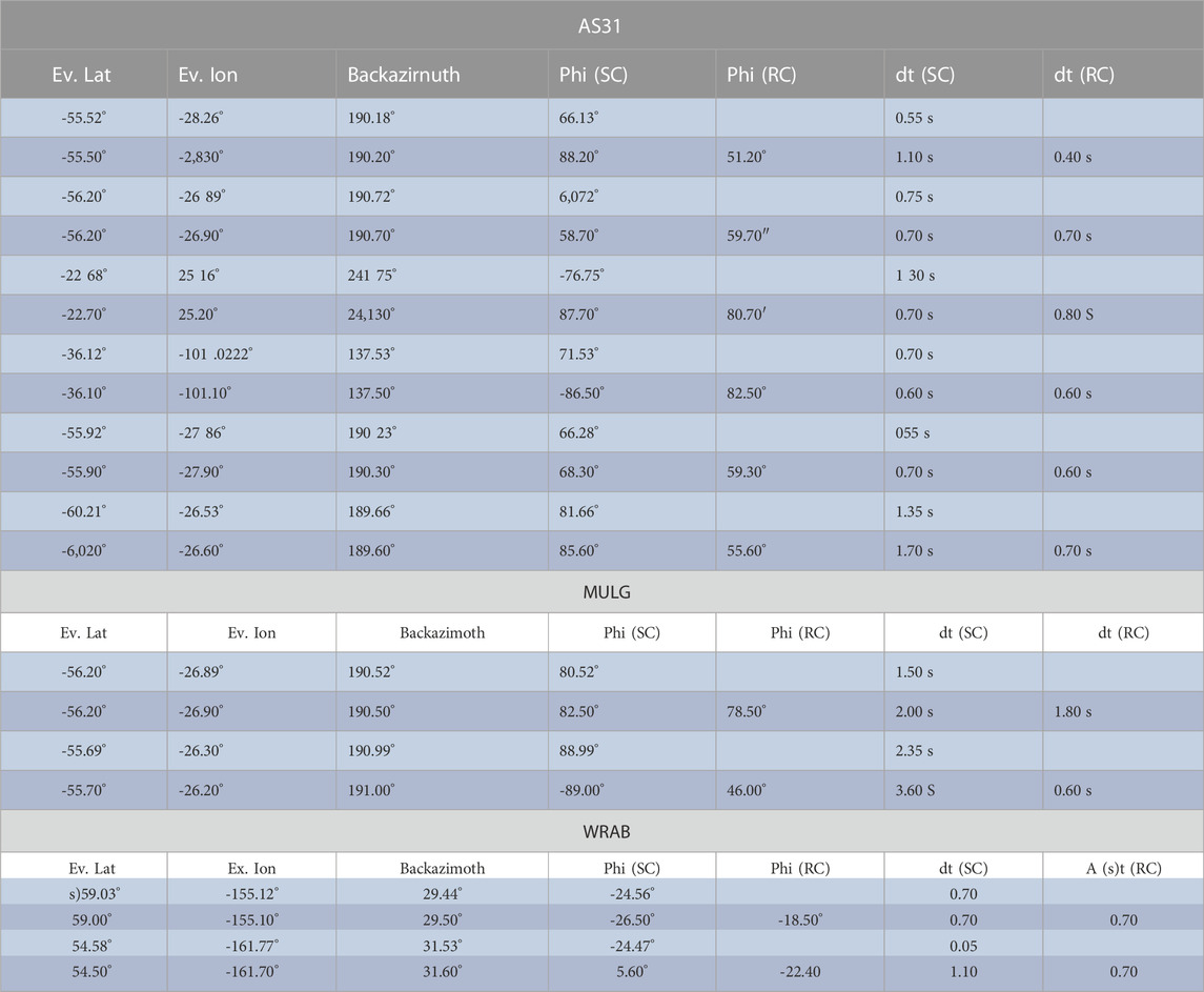
TABLE 3. Comparison of splits calculated by both this study and Eakin et al. (2021). We display the fast direction ϕ) and delay time (dt) for both the minimum energy method (SC) and the rotation correlation method (RC).

A recent study of seismic anisotropy in the Yilgarn Craton (Chen et al., 2021a) used four of the same stations as used in this study (KMBL, MEEK, MORW, and MUN). We had two additional stations within the Yilgarn: BLDU and NWAO, both roughly in line with stations MORW and MUN along the western margin of the craton. Other than KBML, our modeled fast directions are within 20° of average fast directions reported by Chen et al. (2021a), though our averages do not match theirs as well. Disagreement between the two studies could be a result of variations in methodology or events chosen, or the phases used for splitting—Chen et al. (2021a) includes PKS, SKS, SKKS, and SKiKS phases, while this study has mostly SKS and SKKS phases. Modeled delay times are in closer agreement: our delay times range from 0.6 s at station BLDU and MUN to 0.9 s at stations KMBL; Chen et al. (2021a) has a similar range, with 0.5 s at station MUN (south of station BLDU) and 0.7 s at station KMBL. Both studies also suggest general disagreement between plate motion and average fast directions. Despite slight differences, the overall conclusion reached by Chen et al. (2021a) is supported by this study: seismic anisotropy is relatively weak but complex in the Yilgarn Craton, in stark contrast to the exceptionally fast plate motion with strong alignment of asthenospheric seismic anisotropy (Debayle et al., 2005).

Our results are not in good agreement with a previous study examining the structure of southeast Australia (Bello et al., 2019). Both studies report complex splitting parameters that frequently do not mirror plate motion. For all four stations used in both studies (CAN, CNB, TOO, and YNG), our average delay times were significantly lower (1.0 s or less at all stations), whereas Bello et al. (2019) estimate average delay times of greater than 1.0 s. Additionally, fast directions are significantly different at all stations. Bello et al. (2019) used a method similar to the eigenvalue method laid out in Silver and Chan (1991) and also deployed a weighted averaging scheme: this contrasts with our use of the rotation correlation method and no weighting in our averages, which may explain some of the differences.

The differences between our results and those of the other studies indicates the need for a careful analysis of the methodological and data differences in shear wave splitting analysis, particularly in regions such as Australia where seismic anisotropy is vertically stratified and laterally complex. Such complexities are supported by our analysis, specifically at those stations where modelling does not match well with observed fast directions and delay times, and echo the findings of previous studies (e.g., Clitheroe and Van der Hilst, 1998; Heintz and Kennett, 2005). In the remaining sections, we compare our splitting results to constraints from receiver functions and tomography.

4.2 Constraining depth-dependent seismic anisotropy

Shear wave splitting is a path-integrated effect from the core-mantle boundary to the surface, thus it cannot provide firm depth constraints without modeling. However, surface waves are sensitive to changes in seismic anisotropy with depth, thus surface wave tomography can help to provide a lens through which we may be able to better understand our splitting results. A recent global tomography model (Debayle et al., 2016) includes an anisotropic component, which indicates clear changes in anisotropy at short lateral scales, and changes with depth similar to previous tomographic models that indicated a transition from complex anisotropy above 150 km depth to plate motion parallel anisotropy below that (e.g., Debayle et al., 2005; Fishwick and Reading, 2008). Of the 13 stations well modeled by a single layer of anisotropy, seven are within 20° of an E-W orientation, roughly in line with what tomography has indicated. The remaining five and the 16 that cannot be modeled require another explanation such as contributions from multiple layers of anisotropy. We examine other potential causes in Section 4.5.

While we did calculate effective splitting parameters in MSAT (Walker and Wookey, 2012) for a four-layer model using values from the model of Debayle et al. (2016), we determined that, because 45% of stations were well fit by a single layer of anisotropy and the remaining stations were backazimuthally limited, additional complexity was not required and did not warrant comparison to Debayle et al. (2016). This agrees with Eakin et al. (2021), who produced several two-layer models and argued that these models did not fit their results and were not strictly preferred over a one-layer model (wherein seismic anisotropy is present solely in the lithosphere).

One potential explanation for the observed discrepancies in the modeled versus calculated splitting results may come from seismic anisotropy in the lowermost mantle. Contributions to shear wave splitting are assumed to be predominantly within the upper mantle. However, previous studies have indicated the possibility of lowermost mantle seismic anisotropy as a contribution to Australian shear wave splitting results. Özalbey and Chen, 1999 found anomalous waveforms on transverse component seismograms that did not match the predicted shape for upper mantle shear wave splitting (the time-derivative of the radial component), arguing that these anomalous waveforms were likely due to the presence of heterogeneities within the lowermost mantle. More recent studies have also documented lowermost mantle contributions to shear wave splitting across the globe including Africa (Lynner and Long, 2014; Ford et al., 2015), Australia (Creasy et al., 2017), Eurasia (Long and Lynner, 2015); Iceland (Wolf et al., 2019), North America (Lutz et al., 2020). While these studies show a clear presence of seismic anisotropy within the lowermost mantle, results are often heterogeneous and indicate complex seismic anisotropy. Furthermore, constraints on both dominant slip systems and the mechanism of deformation responsible for development of fabric are poorly constrained. In Supplementary Figures S24, we plot our splits at a depth of 2,700 km against the GyPSuM tomography model (Simmons et al., 2010) for the same depth. Splitting parameters exhibit significant heterogeneity across the region, sampling the lowermost mantle over a region of roughly 60° of latitude and 50° of longitude. As such, it is possible that the lowermost mantle has some contribution to our observations of shear wave splitting. Furthermore, while different phases (i.e., SKS, SKKS, and PKS) have very similar paths in the upper mantle, paths diverge significantly in the lowermost mantle: thus, variations in studies may arise as a result of different phases used, especially if seismic anisotropy in the lowermost mantle has a significant contribution. Phases sampling the lowermost mantle coupled with complex upper mantle seismic anisotropy implies that our results are difficult to model or directly interpret without first concretely identifying contributions from each region, which is beyond the scope of the present study.

4.3 Comparison of receiver functions to previous studies

Our Ps receiver functions indicate complex, heterogeneous structure below the Moho. Additionally, we see gradual changes in polarity (i.e., a shift from a positive to a negative pulse) on backazimuthally-binned transverse component receiver functions. In an isotropic, horizontally stratified system, no energy should be present on the transverse component: thus, the presence of such energy (and more specifically polarity changes of said energy) is diagnostic of either anisotropy or dipping layers. Figures 7–10 show these gradual polarity changes; Chen et al. (2021b) examined four stations (KMBL, MEEK, MORW, and MUN) in the Yilgarn craton and performed a harmonic decomposition to constrain anisotropic structure; this method performs a linear regression to constrain polarity flips and divides the receiver function into a combination of sine and cosine terms (Shiomi and Park, 2008). They report clear evidence for two layers of seismic anisotropy at three of these stations (KMBL, MORW, and MUN). At KMBL, Chen et al. (2021b) report three prominent phases potentially associated with dipping structure or seismic anisotropy: at 58, 87, 101 km. At MEEK, they report prominent phases at 74 and 94 km. While Chen et al. (2021b) utilized harmonic decomposition to analyze their receiver functions, rose diagrams can be used to provide a visual representation of similar trends such as seismic anisotropy or dipping layers (Ford et al., 2016; Park and Levin, 2016). In Figure 12, we plot rose diagrams for both stations at corresponding depths: 60, 90, and 100 km ±5 km for KMBL; 75 and 95 km ±5 km for MEEK. While there are polarity flips at station KMBL, these do not match simple two or four-lobed patterns. For station MEEK, polarity flips are much clearer, particularly at 75 km—this matches well with a two-lobed pattern; Chen et al. (2021b) report a dominant contribution to modelled energy from a two-lobed pattern.

FIGURE 12

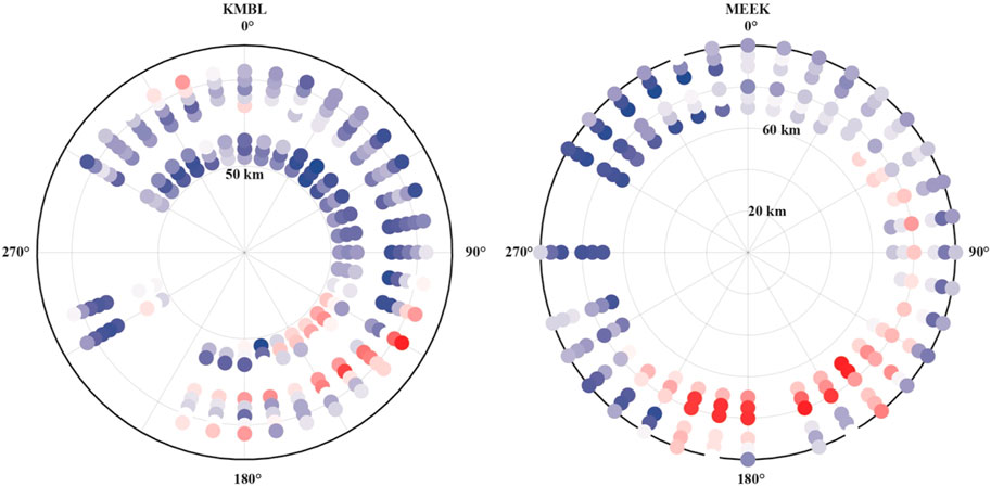
FIGURE 12. Rose diagrams of transverse-component Ps receiver functions for stations used in Chen et al. (2021b) at the depths where their harmonic decomposition indicated polarity changes. Depth increases from zero at the center to 200 km at the edge.

Because receiver functions are sensitive to sharp boundaries, we utilize variations in fast directions with depth from Debayle et al. (2016) to isolate potential depths at which polarity flips on the transverse component of receiver functions might be expected. At station ARMA, there is a single large change in modelled fast direction between 150 km (-89.94°) and 175 km (60.42°). We observe some evidence of a change in polarity at these depths, but these changes are subtle; additionally, this is beneath the predicted depth of the lithosphere-asthenosphere boundary along the eastern margin of the continent. Station BBOO also only has one large change in fast direction, between 70 km (-88.50°) and 90 km (-52.27°) according to Debayle et al. (2016). There are some slight changes in polarity between these two depths in our receiver function results, most consistent with a two-lobed pattern. At station EIDS, there are no large changes in tomographically inferred fast direction within lithospheric depth bounds; while our receiver function results for the station does have some polarity flips, these are not consistent and do not match predicted two-lobed or four-lobed behavior. Tomographically modeled fast directions for station FITZ show a continuous decrease from close to 90° near the surface to a more N-S orientation closer to plate motion at depth; polarity flips are isolated at station FITZ and do not indicate seismic anisotropy. At station KMBL, the model of Debayle et al. (2016) shows only one large jump in fast direction from -23.30° at 70 km to 35.70° at 90 km—our receiver functions for station KMBL do not show corresponding polarity flips. Station MEEK shows modelled fast directions that are roughly consistent at all depths, yet our receiver functions show a two-lobed polarity flip around 80 km. Between 100 km and 125 km, there is a shift in modelled fast direction (56.60°–18.37°) at station OOD. The transverse component receiver function for station OOD does have complex changes in polarity between these two depths, but the pattern is not an obvious two or four-lobed one. Finally, at station WRAB there is also a change in fast direction between 100 km (-57.80°) and 125 km (13.51°); however, while there are polarity flips on the receiver function, they are complex and do not match predicted patterns associated with seismic anisotropy. It is important to note that these comparisons are not direct ones: while receiver functions and surface wave tomography both provide good depth resolution, receiver functions are sensitive to sharp boundaries whereas tomography characterizes changes in volumetric properties. Thus, a lack of explicit agreement between the two methods does not indicate a lack of seismic anisotropy but rather a combination of gradually changing seismic anisotropy constrained by tomography, with fine scale layering of seismic anisotropy imaged by receiver functions.

4.4 Implications for the nature of the Australian lithosphere

Previous geophysical studies have made clear that the Australian continent has a complex lithospheric structure, with variations in the thickness of the lithosphere and its internal properties. Regional tomography models indicate some broad trends within the continent, such as thicker lithosphere with faster wavespeeds in cratonic Australia and thinner lithosphere with slower wavespeeds along the eastern margin (Kennett et al., 2012). Additionally, the lithosphere appears to increase in thickness in a stepwise fashion westward from the Phanerozoic eastern margin. While the lithosphere is generally thicker in the western two-thirds of the continent, there are still significant variations in the depth of the lithosphere-asthenosphere boundary determined from tomography (Kennett et al., 2012). Topography of the lithosphere-asthenosphere boundary may result in complex mantle flow patterns and edge convection, which would produce its own anisotropic signature (e.g., Chen et al., 2021a; Eakin et al., 2021). Global models show the same broad features in Australia (e.g., Debayle et al., 2016).

While the lithosphere-asthenosphere boundary is generally thought of as step-like change in physical properties, some studies have referred to it instead as the lithosphere-asthenosphere transition because (especially in cratons) it is often not a discrete boundary (Mancinelli et al., 2017). One recent study (Yoshizawa and Kennett, 2015) utilized tomography to examine both the lithosphere-asthenosphere transition and radial seismic anisotropy within the Australian upper mantle. This transition occurs at different depths and has variable thickness across the continent: it is thickest and deepest in central Australia in the Proterozoic sutures between cratons; along the eastern margin of the continent the lithosphere-asthenosphere transition is shallower. Trends in radial seismic anisotropy are similar, with the strongest radial seismic anisotropy in the sutures between cratons, decreases in radial seismic anisotropy from the base of the crust to mid-lithospheric depths in the cratons, and strong radial seismic anisotropy in the asthenosphere along the eastern margin. Global models of azimuthal seismic anisotropy (e.g., Debayle et al., 2016) do show variations in seismic anisotropy with depth and across the continent, though these do not mirror major surficial boundaries. Additional constraints on anisotropy come from Quasi-Love wave scattering (Eakin et al., 2021), which indicates anisotropy in Australia is complex and spatially heterogeneous. This scattering is largely in agreement with previous studies indicating anisotropy within Australia is likely fossilized in the lithosphere and linked to the continent’s long tectonic history.

As noted in Section 3.3.2, several of our Ps receiver functions have polarity flips at roughly the same depths as mid-lithospheric discontinuities reported previously (Ford et al., 2010; Birkey et al., 2021). Mid-lithospheric discontinuities seem to be a near-ubiquitous feature of cratonic lithosphere, but their origin is still somewhat unclear. The most common explanations include the presence of current or solidified partial melt, hydrous minerals such as phlogopite, or seismic anisotropy (Selway et al., 2015; Aulbach et al., 2017). Birkey et al. (2021) argue that the most likely explanation for mid-lithospheric discontinuities in Australia is the presence of ancient hydrous minerals; however, they do not rule out the possibility that seismic anisotropy could contribute to the decrease in velocity associated with negative phases observed at mid-lithospheric depths. The polarity flips that we observe occur over 10s of km, which suggests either a thicker layer of seismic anisotropy or a more gradual transition from one fast direction orientation to another. Thus, seismic anisotropy seems likely to not be the sole cause of observed mid-lithospheric discontinuities, although it may provide a contribution, similar to an argument put forward by Ford et al. (2016) for the Wyoming and Superior Cratons. However, it is clear from both this study and previous ones that the Australian lithosphere is anisotropic; such seismic anisotropy must be fossilized within the lithosphere, as there are no obvious explanations for ongoing fabric formation in the lithosphere today. This argument is bolstered by the disagreement between absolute plate motion and the average fast direction of most cratonic stations (except for AS31, MORW, MUN, and WRKA; though an examination of individuals splits makes clear that these stations have significant backazimuthal variability that cannot be explained by plate motion).

In addition to the macroscopic alignment of intrinsically seismically anisotropic minerals, the layering of media with different material properties can also produce seismic anisotropy. Earthquakes originating from Australia have complex high-frequency body-wave codas; Kennett et al. (2017) argue that this is due to multi-scale heterogeneity (i.e., layering occurs at multiple scales). Such heterogeneity could contribute to the complex splitting patterns that are observed in Australia and could be linked to the formation and evolution of the lithosphere.

4.5 Relating observed seismic anisotropy to geologic structure

Simple interpretations of the seismic anisotropy present within the Australian lithosphere are difficult, and readers should be cautious of shear wave splitting results for two primary reasons. First, as noted in this study, there are discrepancies between various published shear wave splitting studies for Australia. As noted above, there are some differences in phases used and methodology: we report our results from the rotation correlation method, which has been shown to have a systematic 45° misorientation in fast direction for near-null backazimuths (Wüstefeld and Bokelmann, 2007; Eakin et al., 2019). Modeling of this sawtooth pattern does resolve some differences, but others remain, underscoring the complexity of seismic anisotropy in the region. Second, contributions to shear wave splitting from the lowermost mantle cannot be ruled out, implying that observed fast directions may be the result of splitting throughout the mantle. This second point is an emerging issue in the calculation of shear wave splitting globally.

Caveats aside, this last section focuses on comparing shear wave splitting and receiver function results from a selected number of stations to the observed geology and inferred tectonic history of the Australian continent. Importantly, while seismic anisotropy can be correlated to specific processes in regions of active tectonism, this is less intuitive for cratons as there may be multiple layers of anisotropy that result in a complex signal not easily linked to specific events. As noted elsewhere, previous studies have indicated the presence of multiple layers of seismic anisotropy within the Australian lithosphere (e.g., Simons et al., 2002). Multiple layers of anisotropy may be a good candidate explanation for many of our results, though there is no apparent reason for the lithosphere of the entire continent to have a roughly consistent fast direction. Additionally, many tectonic events in the Precambrian are poorly constrained, making it difficult to definitively argue for any one cause of the anisotropy we observe (e.g., Chen et al., 2021a).

4.5.1 North Australian Craton

For station COEN (in the Coen Inlier), we report an average fast direction of -28.7°, which deviates from the more N-S direction of plate motion. However, there is evidence for NNW-SSE directed shortening at ∼1.65 Ga (Cihan et al., 2006), which could explain our results. Most individual splits are roughly parallel to the predicted direction of shortening, except for a few results that are almost perpendicular (these come from a limited backazimuthal range, however).

At station FITZ, our average fast direction is 62.7°, with individual splits roughly oriented the same direction. These measurements are subparallel to stress orientations in that part of the NAC (the Canning Basin; Bailey et al., 2021)—some studies have indicated a link between presently measured stress and anisotropy; however, we note that stress here is determined from borehole measurements, which only sample the shallow crust. While this region has relatively thick sedimentary cover (several kilometers in some spots), it is not likely that crustal anisotropy alone would be enough to produce the strength of splitting we observe here. We do note, however, that transverse component receiver functions exhibit some polarity flips above the Moho (at ∼20 km for instance), which may indicate a crustal contribution to anisotropy.

Stations KDU and MTN are both in the Pine Creek Inlier and have similar average fast directions (32.5° and 18.5°, respectively). Near MTN, there are several faults with strikes subparallel to its average fast direction (Needham et al., 1988). There is some evidence from ocean basins that faults can induce seismic anisotropy parallel to their strike (Faccenda et al., 2008), but this may not be directly applicable to continental settings given the thicker crust and mantle lithosphere. Additionally, individual splitting measurements at MTN vary quite a bit, so while the average fast direction mirrors the strike of local faults, this may not be the cause of the anisotropy. KDU is farther from these faults and is well modeled by a single layer of anisotropy oriented at 71°, implying that anisotropy there cannot be explained by faulting.

KNRA may be the strongest candidate for a station with anisotropy that is well explained by tectonic history. Its modeled fast direction (38°) is similar to the strike of the Halls Creek Orogen (though the station is north of known exposures), and there is evidence for west-dipping subduction in the Proterozoic (Sheppard et al., 1999); fast directions are expected to be trench parallel in such settings, which may explain the average fast direction we report. Individual fast directions do have more variability but are in general similar to the strike of the Halls Creek Orogen.

The average fast direction at WRAB deviates slightly from the trend of the Tenant Creek Inlier. However, one grouping of individual fast directions does mirror the trend, similar to what Eakin et al. (2021) reported; there is another that is roughly perpendicular to that first group. Transverse component receiver functions show some possible polarity flips at lithospheric mantle depths for WRAB, though as noted elsewhere these are not easily modelled. This may indicate complex seismic anisotropy at depth that contributes to the variations in fast direction.

4.5.2 South Australian Craton

We do not find compelling evidence that our results are well explained by surface geologic features, which is not surprising given the Archean age of parts of the craton. Averaged splits at seven stations trend NE-SW, which does not mirror the boundaries of the SAC or any of its components—the one exception being at station FORT where the average fast direction does trend similar to the boundary between the SAC and the Albany-Fraser Orogen to its west and may be explained by compression during Orogenesis.

4.5.3 West Australian Craton

One important feature of the WAC is that some tomographic studies have imaged slightly thinner lithosphere along the western margins of the craton than other portions of cratonic Australia (e.g. Yoshizawa and Kennett, 2015). This is corroborated by Birkey et al. (2021), who saw evidence for the lithosphere-asthenosphere boundary along the western margin of the continent. If the western margin is indeed thinner than central Australia, this could produce edge-driven convection. In turn, this would result in the development of new seismically anisotropic fabrics that may contribute to the shear wave splitting we observe. As many of the stations in the WAC exhibit complex splitting behavior, multiple contributions to the signal are not unexpected. One station that may have a tectonic explanation for its anisotropic signal is MEEK, with a modeled fast direction of 87°. This is roughly parallel to the Capricorn Orogen to its north.

4.5.4 Phanerozoic Australia

Many of the stations in Phanerozoic Australia have average fast directions close to plate motion (roughly N-S), which may be expected for thinner lithosphere with an anisotropic signal dominated by shear at the base of the plate. Two clear exceptions to this are EIDS and TOO, though this seems likely to be a result of more splits coming from backazimuths with fast directions that differ from APM as there are splits at each station that do match APM.

Stations CAN, CNB, and YNG are all in the Lachlan Orogen, with average fast directions that are roughly parallel to geologic features of the orogen in that region as well APM. However, individual splitting measurements vary significantly by backazimuth, with few mirroring plate motion. A previous receiver function study (Girardin and Farra, 1998) did find two layers of anisotropy beneath CAN: an upper layer oriented E-W (possibly linked to E-W extension), and a lower layer oriented N-S (most likely linked to plate motion). This layered anisotropy could explain the results that we observe at all three stations.

5 Conclusion

We present shear wave splitting and Ps receiver function results from permanent stations across the Australian continent. Importantly, both methods indicate that anisotropy within the Australian lithosphere is complex. While average fast directions are similar to absolute plate motion, there is variability in fast direction with backazimuth (diagnostic of said complexity). Even at stations within Phanerozoic Australia, we observe evidence for complex anisotropy from shear wave splitting, suggesting that in many cases multiple layers of seismic anisotropy may be required. However, shear wave splitting cannot directly provide depth constraints—for this we instead rely on Ps receiver functions. These display some changes in polarity on transverse components over 10s of kilometers, suggesting that any changes in seismic anisotropy do not occur as sharp interfaces. Ps receiver functions presented here are also in agreement with previously published Sp receiver functions across Australia, particularly at mid-lithospheric depths. Though results from both methods warrant caution in interpretation, the ancient lithosphere of the Australian continent likely preserves anisotropic fabric related to its formation and evolution, with minimal contributions from present-day plate motion.

Data availability statement

The original contributions presented in the study are included in the article/Supplementary Material, further inquiries can be directed to the corresponding author.

Author contributions

AB performed analysis, wrote original draft, produced figures, and edited drafts. HAF conceptualized the study, secured funding, and edited drafts.

Acknowledgments

We would like to thank Maureen Long and Megan Anderson for their contribution to the formulation of this project. We also thank three reviewers for their helpful suggestions. All data from the following networks were freely and publicly accessed using the IRIS DMC: AU (DOI https://dx.doi.org/10.26186/144675); G (DOI http://doi.org/10.18715/GEOSCOPE.G); II (DOI https://doi.org/10.7914/SN/II); IU (DOI https://doi.org/10.7914/SN/IU).

Conflict of interest

The authors declare that the research was conducted in the absence of any commercial or financial relationships that could be construed as a potential conflict of interest.

Publisher’s note

All claims expressed in this article are solely those of the authors and do not necessarily represent those of their affiliated organizations, or those of the publisher, the editors and the reviewers. Any product that may be evaluated in this article, or claim that may be made by its manufacturer, is not guaranteed or endorsed by the publisher.

Supplementary material

The Supplementary Material for this article can be found online at: https://www.frontiersin.org/articles/10.3389/feart.2022.1055480/full#supplementary-material

References

Aulbach, S., Massuyeau, M., and Gaillard, F. (2017). Origins of cratonic mantle discontinuities: A view from petrology, geochemistry and thermodynamic models. Lithos 268, 364–382. doi:10.1016/j.lithos.2016.11.004

CrossRef Full Text | Google Scholar

Ba, K., Gao, S. S., Liu, K. H., Kong, F., and Song, J. (2020). Receiver function imaging of the 410 and 660 km discontinuities beneath the Australian continent. Geophys. J. Int. 220 (3), 1481–1490. doi:10.1093/gji/ggz525

CrossRef Full Text | Google Scholar

Bailey, A. H. E., Jarrett, A. J. M., Tenthorey, E., and Henson, P. A. (2021). Understanding present-day stress in the onshore Canning Basin of western Australia. Aust. J. Earth Sci. 68 (6), 818–838. doi:10.1080/08120099.2021.1879265

CrossRef Full Text | Google Scholar

Bedrosian, P. A., and Finn, C. A. (2021). When Wyoming became superior: Oblique convergence along the southern trans-hudson orogen. Geophys. Res. Lett. 48 (13), e2021GL092970. doi:10.1029/2021gl092970

CrossRef Full Text | Google Scholar

Bello, M., Cornwell, D. G., Rawlinson, N., and Reading, A. M. (2019). Insights into the structure and dynamics of the upper mantle beneath Bass Strait, southeast Australia, using shear wave splitting. Phys. Earth Planet. Interiors 289, 45–62. doi:10.1016/j.pepi.2019.02.002

CrossRef Full Text | Google Scholar

Birkey, A., Ford, H. A., Dabney, P., and Goldhagen, G. (2021). The lithospheric architecture of Australia from seismic receiver functions. J. Geophys. Res. Solid Earth 126 (4), e2020JB020999. doi:10.1029/2020jb020999

CrossRef Full Text | Google Scholar

Bostock, M. G. (1997). Anisotropic upper-mantle stratigraphy and architecture of the Slave craton. Nature 390 (6658), 392–395. doi:10.1038/37102

CrossRef Full Text | Google Scholar

Bostock, M. G. (1998). Mantle stratigraphy and evolution of the Slave province. J. Geophys. Res. Solid Earth 103 (B9), 21183–21200. doi:10.1029/98jb01069

CrossRef Full Text | Google Scholar

Bowman, J. R., and Ando, M. (1987). Shear-wave splitting in the upper-mantle wedge above the Tonga subduction zone. Geophys. J. Int. 88 (1), 25–41. doi:10.1111/j.1365-246x.1987.tb01367.x

CrossRef Full Text | Google Scholar

Brownlee, S. J., Schulte Pelkum, V., Raju, A., Mahan, K., Condit, C., and Orlandini, O. F. (2017). Characteristics of deep crustal seismic anisotropy from a compilation of rock elasticity tensors and their expression in receiver functions. Tectonics 36 (9), 1835–1857. doi:10.1002/2017tc004625

CrossRef Full Text | Google Scholar

Chen, X., Levin, V., Yuan, H., Klaser, M., and Li, Y. (2021b). Seismic anisotropic layering in the Yilgarn and Superior cratonic lithosphere. J. Geophys. Res. Solid Earth 126 (8), e2020JB021575. doi:10.1029/2020jb021575

CrossRef Full Text | Google Scholar

Chen, X., Levin, V., and Yuan, H. (2021a). Small shear wave splitting delays suggest weak anisotropy in cratonic mantle lithosphere. Geophys. Res. Lett. 48 (16), e2021GL093861. doi:10.1029/2021gl093861

CrossRef Full Text | Google Scholar

Chen, X., Li, Y., and Levin, V. (2018). Shear wave splitting beneath eastern north American continent: Evidence for a multilayered and laterally variable anisotropic structure. Geochem. Geophys. Geosystems 19 (8), 2857–2871. doi:10.1029/2018gc007646

CrossRef Full Text | Google Scholar

Cihan, M., Evins, P., Lisowiec, N., and Blake, K. (2006). Time constraints on deformation and metamorphism from EPMA dating of monazite in the Proterozoic Robertson River Metamorphics, NE Australia. Precambrian Res. 145 (1-2), 1–23. doi:10.1016/j.precamres.2005.11.009

CrossRef Full Text | Google Scholar

Clarke, G. L., Sun, S. S., and White, R. W. (1995). Grenville-age belts and associated older terranes in Australia and Antarctica. AGSO J. Aust. Geol. Geophys. 16 (1), 25–40.

Google Scholar

Clitheroe, G., and Van Der Hilst, R. D. (1998). Complex anisotropy in the Australian lithosphere from shear-wave splitting in broad-band SKS records. Geodyn. Ser. 26, 73.

CrossRef Full Text | Google Scholar

Collins, W. J., and Shaw, R. D. (1995). Geochronological constraints on orogenic events in the Arunta inlier: A review. Precambrian Res. 71 (1-4), 315–346. doi:10.1016/0301-9268(94)00067-2

CrossRef Full Text | Google Scholar

Conder, J. A. (2007). Dynamically driven mantle flow and shear wave splitting asymmetry across the EPR, MELT area. Geophys. Res. Lett. 34 (16). doi:10.1029/2007gl030832

CrossRef Full Text | Google Scholar

Coney, P. J., Edwards, A., Hine, R., Morrison, F., and Windrim, D. (1990). The regional tectonics of the Tasman orogenic system, eastern Australia. J. Struct. Geol. 12 (5-6), 519–543. doi:10.1016/0191-8141(90)90071-6

CrossRef Full Text | Google Scholar

Creasy, N., Long, M. D., and Ford, H. A. (2017). Deformation in the lowermost mantle beneath Australia from observations and models of seismic anisotropy. J. Geophys. Res. Solid Earth 122 (7), 5243–5267. doi:10.1002/2016jb013901

CrossRef Full Text | Google Scholar

Debayle, E., Dubuffet, F., and Durand, S. (2016). An automatically updated S-wave model of the upper mantle and the depth extent of azimuthal anisotropy. Geophys. Res. Lett. 43 (2), 674–682. doi:10.1002/2015gl067329

CrossRef Full Text | Google Scholar

Debayle, E., and Kennett, B. L. N. (2000). The Australian continental upper mantle: Structure and deformation inferred from surface waves. J. Geophys. Res. Solid Earth 105 (B11), 25423–25450. doi:10.1029/2000jb900212

CrossRef Full Text | Google Scholar

Debayle, E., Kennett, B., and Priestley, K. (2005). Global azimuthal seismic anisotropy and the unique plate-motion deformation of Australia. Nature 433 (7025), 509–512. doi:10.1038/nature03247

PubMed Abstract | CrossRef Full Text | Google Scholar

Debayle, E. (1999). SV-Wave azimuthal anisotropy in the Australian upper mantle: Preliminary results from automated Rayleigh waveform inversion. Geophys. J. Int. 137 (3), 747–754. doi:10.1046/j.1365-246x.1999.00832.x

CrossRef Full Text | Google Scholar

Deng, J., Long, M. D., Creasy, N., Wagner, L., Beck, S., Zandt, G., et al. (2017). Lowermost mantle anisotropy near the eastern edge of the pacific LLSVP: Constraints from SKS–SKKS splitting intensity measurements. Geophys. J. Int. 210 (2), 774–786. doi:10.1093/gji/ggx190

CrossRef Full Text | Google Scholar

Direen, N. G., and Crawford, A. J. (2003). The tasman line: Where is it, what is it, and is it Australia's rodinian breakup boundary? Aust. J. Earth Sci. 50 (4), 491–502. doi:10.1046/j.1440-0952.2003.01005.x

CrossRef Full Text | Google Scholar

Du Frane, W. L., Roberts, J. J., Toffelmier, D. A., and Tyburczy, J. A. (2005). Anisotropy of electrical conductivity in dry olivine. Geophys. Res. Lett. 32 (24), L24315. doi:10.1029/2005gl023879

CrossRef Full Text | Google Scholar

Eakin, C. M., Flashman, C., and Agrawal, S. (2021). Seismic anisotropy beneath central Australia: A record of ancient lithospheric deformation. Tectonophysics 820, 229123. doi:10.1016/j.tecto.2021.229123

CrossRef Full Text | Google Scholar

Eakin, C. M., and Long, M. D. (2013). Complex anisotropy beneath the Peruvian flat slab from frequency-dependent, multiple-phase shear wave splitting analysis. J. Geophys. Res. Solid Earth 118 (9), 4794–4813. doi:10.1002/jgrb.50349

CrossRef Full Text | Google Scholar

Eakin, C. M., Wirth, E. A., Wallace, A., Ulberg, C. W., Creager, K. C., and Abers, G. A. (2019). SKS splitting beneath Mount St. Helens: Constraints on subslab mantle entrainment. Geochem. Geophys. Geosystems 20 (8), 4202–4217. doi:10.1029/2019gc008433

CrossRef Full Text | Google Scholar

Faccenda, M., Burlini, L., Gerya, T. V., and Mainprice, D. (2008). Fault-induced seismic anisotropy by hydration in subducting oceanic plates. Nature 455 (7216), 1097–1100. doi:10.1038/nature07376

CrossRef Full Text | Google Scholar

Fishwick, S., and Reading, A. M. (2008). Anomalous lithosphere beneath the proterozoic of Western and central Australia: A record of continental collision and intraplate deformation? Precambrian Res. 166 (1-4), 111–121. doi:10.1016/j.precamres.2007.04.026

CrossRef Full Text | Google Scholar

Ford, H. A., Fischer, K. M., Abt, D. L., Rychert, C. A., and Elkins-Tanton, L. T. (2010). The lithosphere–asthenosphere boundary and cratonic lithospheric layering beneath Australia from Sp wave imaging. Earth Planet. Sci. Lett. 300 (3-4), 299–310. doi:10.1016/j.epsl.2010.10.007

CrossRef Full Text | Google Scholar

Ford, H. A., Long, M. D., He, X., and Lynner, C. (2015). Lowermost mantle flow at the eastern edge of the african large low shear velocity province. Earth Planet. Sci. Lett. 420, 12–22. doi:10.1016/j.epsl.2015.03.029

CrossRef Full Text | Google Scholar

Ford, H. A., Long, M. D., and Wirth, E. A. (2016). Midlithospheric discontinuities and complex anisotropic layering in the mantle lithosphere beneath the Wyoming and Superior Provinces. J. Geophys. Res. Solid Earth 121 (9), 6675–6697. doi:10.1002/2016jb012978

CrossRef Full Text | Google Scholar

Foster, D. A., and Gray, D. R. (2000). Evolution and structure of the lachlan fold belt (orogen) of eastern Australia. Annu. Rev. Earth Planet. Sci. 28 (1), 47–80. doi:10.1146/annurev.earth.28.1.47

CrossRef Full Text | Google Scholar

Girardin, N., and Farra, V. (1998). Azimuthal anisotropy in the upper mantle from observations ofP-to-S converted phases: Application to southeast Australia. Geophys. J. Int. 133, 615–629. doi:10.1046/j.1365-246x.1998.00525.x

CrossRef Full Text | Google Scholar

Gripp, A. E., and Gordon, R. G. (2002). Young tracks of hotspots and current plate velocities. Geophys. J. Int. 150 (2), 321–361. doi:10.1046/j.1365-246x.2002.01627.x

CrossRef Full Text | Google Scholar

Heintz, M., and Kennett, B. L. (2005). Continental scale shear wave splitting analysis: Investigation of seismic anisotropy underneath the Australian continent. Earth Planet. Sci. Lett. 236 (1-2), 106–119. doi:10.1016/j.epsl.2005.05.003

CrossRef Full Text | Google Scholar

Heintz, M., and Kennett, B. L. (2006). The apparently isotropic Australian upper mantle. Geophys. Res. Lett. 33 (15), L15319. doi:10.1029/2006gl026401

CrossRef Full Text | Google Scholar

Hopper, E., and Fischer, K. M. (2015). The meaning of midlithospheric discontinuities: A case study in the northern us craton. Geochem. Geophys. Geosystems 16 (12), 4057–4083. doi:10.1002/2015gc006030

CrossRef Full Text | Google Scholar

Hopper, E., Fischer, K. M., Wagner, L. S., and Hawman, R. B. (2017). Reconstructing the end of the Appalachian orogeny. Geology 45 (1), 15–18. doi:10.1130/g38453.1

CrossRef Full Text | Google Scholar

Jordan, T. H. (1975). The continental tectosphere. Rev. Geophys. 13 (3), 1–12. doi:10.1029/rg013i003p00001

CrossRef Full Text | Google Scholar

Karato, S. I., Jung, H., Katayama, I., and Skemer, P. (2008). Geodynamic significance of seismic anisotropy of the upper mantle: New insights from laboratory studies. Annu. Rev. Earth Planet. Sci. 36 (1), 59–95. doi:10.1146/annurev.earth.36.031207.124120

CrossRef Full Text | Google Scholar

Kennett, B. L., Fichtner, A., Fishwick, S., and Yoshizawa, K. (2013). Australian seismological reference model (AuSREM): Mantle component. Geophys. J. Int. 192 (2), 871–887. doi:10.1093/gji/ggs065

CrossRef Full Text | Google Scholar

Kennett, B. L. N., and Abdullah, A. (2011). Seismic wave attenuation beneath the Australasian region. Aust. J. Earth Sci. 58 (3), 285–295. doi:10.1080/08120099.2011.550318

CrossRef Full Text | Google Scholar

Kennett, B. L. N., and Salmon, M. (2012). AuSREM: Australian seismological reference model. Aust. J. Earth Sci. 59 (8), 1091–1103. doi:10.1080/08120099.2012.736406

CrossRef Full Text | Google Scholar

Kennett, B. L. N., Salmon, M., Saygin, E., and Group, A. W. (2012). AusMoho: The variation of Moho depth in Australia. Geophys. J. Int. 187 (2), 946–958. doi:10.1111/j.1365-246x.2011.05194.x

CrossRef Full Text | Google Scholar

Kennett, B. L. N., Yoshizawa, K., and Furumura, T. (2017). Interactions of multi-scale heterogeneity in the lithosphere: Australia. Tectonophysics 717, 193–213. doi:10.1016/j.tecto.2017.07.009

CrossRef Full Text | Google Scholar

Kumazawa, M., and Anderson, O. L. (1969). Elastic moduli, pressure derivatives, and temperature derivatives of single-crystal olivine and single-crystal forsterite. J. Geophys. Res. 74 (25), 5961–5972. doi:10.1029/jb074i025p05961

CrossRef Full Text | Google Scholar

Laske, G., Masters, G., Ma, Z., and Pasyanos, M. (2013). Update on CRUST1. 0—a 1-degree global model of Earth’s crust. Geophys. Res. Abstr. 15, 2658.

Google Scholar

Levin, V., and Park, J. (1997). P-SH conversions in a flat-layered medium with anisotropy of arbitrary orientation. Geophys. J. Int. 131 (2), 253–266. doi:10.1111/j.1365-246x.1997.tb01220.x

CrossRef Full Text | Google Scholar

Li, Z. X. (2000). Palaeomagnetic evidence for unification of the North and West Australian cratons by ca. 1.7 Ga: New results from the kimberley basin of northwestern Australia. Geophys. J. Int. 142 (1), 173–180. doi:10.1046/j.1365-246x.2000.00143.x

CrossRef Full Text | Google Scholar

Liu, G., Persaud, P., and Clayton, R. W. (2018). Structure of the northern Los Angeles basins revealed in teleseismic receiver functions from short-term nodal seismic arrays. Seismol. Res. Lett. 89 (5), 1680–1689. doi:10.1785/0220180071

CrossRef Full Text | Google Scholar

Long, M. D., Ford, H. A., Abrahams, L., and Wirth, E. A. (2017). The seismic signature of lithospheric deformation beneath eastern North America due to Grenville and Appalachian orogenesis. Lithosphere 9 (6), 987–1001. doi:10.1130/l660.1

CrossRef Full Text | Google Scholar

Long, M. D., and Lynner, C. (2015). Seismic anisotropy in the lowermost mantle near the Perm Anomaly. Geophys. Res. Lett. 42 (17), 7073–7080. doi:10.1002/2015gl065506

CrossRef Full Text | Google Scholar

Long, M. D., and Silver, P. G. (2008). The subduction zone flow field from seismic anisotropy: A global view. science 319 (5861), 315–318. doi:10.1126/science.1150809

PubMed Abstract | CrossRef Full Text | Google Scholar

Lutz, K. A., Long, M. D., Creasy, N., and Deng, J. (2020). Seismic anisotropy in the lowermost mantle beneath North America from SKS-SKKS splitting intensity discrepancies. Phys. Earth Planet. Interiors 305, 106504. doi:10.1016/j.pepi.2020.106504

CrossRef Full Text | Google Scholar

Lynner, C., and Long, M. D. (2014). Lowermost mantle anisotropy and deformation along the boundary of the African LLSVP. Geophys. Res. Lett. 41 (10), 3447–3454. doi:10.1002/2014gl059875

CrossRef Full Text | Google Scholar

Mancinelli, N. J., Fischer, K. M., and Dalton, C. A. (2017). How sharp is the cratonic lithosphere-asthenosphere transition? Geophys. Res. Lett. 44 (20), 10,189–10,197. doi:10.1002/2017gl074518

CrossRef Full Text | Google Scholar

Marshak, S., and Flöttmann, T. (1996). Structure and origin of the fleurieu and nackara arcs in the adelaide fold-thrust belt, south Australia: Salient and recess development in the delamerian orogen. J. Struct. Geol. 18 (7), 891–908. doi:10.1016/0191-8141(96)00016-8

CrossRef Full Text | Google Scholar

Murray, C. G., and Kirkegaard, A. G. (1978). The Thomson orogen of the tasman orogenic zone. Tectonophysics 48 (3-4), 299–325. doi:10.1016/0040-1951(78)90122-1

CrossRef Full Text | Google Scholar

Musacchio, G., White, D. J., Asudeh, I., and Thomson, C. J. (2004). Lithospheric structure and composition of the Archean Western Superior Province from seismic refraction/wide-angle reflection and gravity modeling. J. Geophys. Res. Solid Earth 109 (B3), B03304. doi:10.1029/2003jb002427

CrossRef Full Text | Google Scholar

Myers, J. S., Shaw, R. D., and Tyler, I. M. (1996). Tectonic evolution of proterozoic Australia. Tectonics 15 (6), 1431–1446. doi:10.1029/96tc02356

CrossRef Full Text | Google Scholar

Needham, R. S., Stuart-Smith, P. G., and Page, R. W. (1988). Tectonic evolution of the pine Creek inlier, northern territory. Precambrian Res. 40, 543–564. doi:10.1016/0301-9268(88)90084-8

CrossRef Full Text | Google Scholar

Özalaybey, S., and Chen, W. P. (1999). Frequency-dependent analysis of SKS/SKKS waveforms observed in Australia: Evidence for null birefringence. Phys. earth Planet. interiors 114 (3-4), 197–210. doi:10.1016/s0031-9201(99)00058-8

CrossRef Full Text | Google Scholar

Park, J., and Levin, V. (2016). Anisotropic shear zones revealed by backazimuthal harmonics of teleseismic receiver functions. Geophys. Suppl. Mon. notices R. Astronomical Soc. 207 (2), 1216–1243. doi:10.1093/gji/ggw323

CrossRef Full Text | Google Scholar

Peterson, J. R. (1993). Observations and modeling of seismic background noise (No. 93-322). Albuquerque, NM: US Geological Survey.

Google Scholar

Reading, A. M., and Kennett, B. L. N. (2003). Lithospheric structure of the Pilbara craton, Capricorn orogen and northern Yilgarn craton, western Australia, from teleseismic receiver functions. Aust. J. Earth Sci. 50 (3), 439–445. doi:10.1046/j.1440-0952.2003.01003.x

CrossRef Full Text | Google Scholar

Rychert, C. A., and Shearer, P. M. (2009). A global view of the lithosphere-asthenosphere boundary. Science 324 (5926), 495–498. doi:10.1126/science.1169754

PubMed Abstract | CrossRef Full Text | Google Scholar

Salmon, M., Kennett, B. L. N., and Saygin, E. (2013). Australian seismological reference model (AuSREM): Crustal component. Geophys. J. Int. 192 (1), 190–206. doi:10.1093/gji/ggs004

CrossRef Full Text | Google Scholar

Savage, M. K. (1999). Seismic anisotropy and mantle deformation: What have we learned from shear wave splitting? Rev. Geophys. 37 (1), 65–106. doi:10.1029/98rg02075

CrossRef Full Text | Google Scholar

Saygin, E., and Kennett, B. L. N. (2012). Crustal structure of Australia from ambient seismic noise tomography. J. Geophys. Res. Solid Earth 117 (B1). doi:10.1029/2011jb008403

CrossRef Full Text | Google Scholar

Schulte-Pelkum, V., and Mahan, K. H. (2014). A method for mapping crustal deformation and anisotropy with receiver functions and first results from USArray. Earth Planet. Sci. Lett. 402, 221–233. doi:10.1016/j.epsl.2014.01.050

CrossRef Full Text | Google Scholar

Selway, K. (2018). Electrical discontinuities in the continental lithosphere imaged with magnetotellurics. Lithospheric discontinuities, 89–109. doi:10.1002/9781119249740.ch5

CrossRef Full Text | Google Scholar

Selway, K., Ford, H., and Kelemen, P. (2015). The seismic mid-lithosphere discontinuity. Earth Planet. Sci. Lett. 414, 45–57. doi:10.1016/j.epsl.2014.12.029

CrossRef Full Text | Google Scholar

Sheppard, S., Tyler, I. M., Griffin, T. J., and Taylor, W. R. (1999). Palaeoproterozoic subduction-related and passive margin basalts in the Halls Creek Orogen, northwest Australia. Aust. J. Earth Sci. 46 (5), 679–690. doi:10.1046/j.1440-0952.1999.00737.x

CrossRef Full Text | Google Scholar

Shiomi, K., and Park, J. (2008). Structural features of the subducting slab beneath the Kii Peninsula, central Japan: Seismic evidence of slab segmentation, dehydration, and anisotropy. J. Geophys. Res. Solid Earth 113 (B10), B10318. doi:10.1029/2007jb005535

CrossRef Full Text | Google Scholar

Silver, P. G., and Chan, W. W. (1991). Shear wave splitting and subcontinental mantle deformation. J. Geophys. Res. Solid Earth 96 (B10), 16429–16454. doi:10.1029/91jb00899

CrossRef Full Text | Google Scholar

Simmons, N. A., Forte, A. M., Boschi, L., and Grand, S. P. (2010). GyPSuM: A joint tomographic model of mantle density and seismic wave speeds. J. Geophys. Res. Solid Earth 115 (B12), B12310. doi:10.1029/2010jb007631

CrossRef Full Text | Google Scholar

Simons, F. J., Van Der Hilst, R. D., Montagner, J. P., and Zielhuis, A. (2002). Multimode Rayleigh wave inversion for heterogeneity and azimuthal anisotropy of the Australian upper mantle. Geophys. J. Int. 151 (3), 738–754. doi:10.1046/j.1365-246x.2002.01787.x

CrossRef Full Text | Google Scholar

Smithies, R. H., and Bagas, L. (1997). High pressure amphibolite-granulite facies metamorphism in the Paleoproterozoic Rudall Complex, central Western Australia. Precambrian Res. 83 (4), 243–265. doi:10.1016/s0301-9268(96)00051-4

CrossRef Full Text | Google Scholar

Tesauro, M., Kaban, M. K., and Aitken, A. R. (2020). Thermal and compositional anomalies of the Australian upper mantle from seismic and gravity data. Geochem. Geophys. Geosystems 21 (11), e2020GC009305. doi:10.1029/2020gc009305

CrossRef Full Text | Google Scholar

Vauchez, A., Tommasi, A., Barruol, G., and Maumus, J. (2000). Upper mantle deformation and seismic anisotropy in continental rifts. Phys. Chem. Earth, Part A Solid Earth Geodesy 25 (2), 111–117. doi:10.1016/s1464-1895(00)00019-3

CrossRef Full Text | Google Scholar

Vauchez, A., Tommasi, A., and Barruol, G. (1998). Rheological heterogeneity, mechanical anisotropy and deformation of the continental lithosphere. Tectonophysics 296 (1-2), 61–86. doi:10.1016/s0040-1951(98)00137-1

CrossRef Full Text | Google Scholar

Vinnik, L. P., Makeyeva, L. I., Milev, A., and Usenko, A. Y. (1992). Global patterns of azimuthal anisotropy and deformations in the continental mantle. Geophys. J. Int. 111 (3), 433–447. doi:10.1111/j.1365-246x.1992.tb02102.x

CrossRef Full Text | Google Scholar

Walker, A. M., and Wookey, J. (2012). MSAT—a new toolkit for the analysis of elastic and seismic anisotropy. Comput. Geosciences 49, 81–90. doi:10.1016/j.cageo.2012.05.031

CrossRef Full Text | Google Scholar

Walker, K. T., Nyblade, A. A., Klemperer, S. L., Bokelmann, G. H., and Owens, T. J. (2004). On the relationship between extension and anisotropy: Constraints from shear wave splitting across the East African Plateau. J. Geophys. Res. Solid Earth 109 (B8). doi:10.1029/2003jb002866

CrossRef Full Text | Google Scholar

Wang, L., Hitchman, A. P., Ogawa, Y., Siripunvaraporn, W., Ichiki, M., and Fuji-Ta, K. (2014). A 3-D conductivity model of the Australian continent using observatory and magnetometer array data. Geophys. J. Int. 198 (2), 1143–1158. doi:10.1093/gji/ggu188

CrossRef Full Text | Google Scholar

Wirth, E. A., and Long, M. D. (2014). A contrast in anisotropy across mid-lithospheric discontinuities beneath the central United States—a relic of craton formation. Geology 42 (10), 851–854. doi:10.1130/g35804.1

CrossRef Full Text | Google Scholar

Wirth, E. A., and Long, M. D. (2012). Multiple layers of seismic anisotropy and a low-velocity region in the mantle wedge beneath Japan: Evidence from teleseismic receiver functions. Geochem. Geophys. Geosystems 13 (8). doi:10.1029/2012gc004180

CrossRef Full Text | Google Scholar

Wolf, J., Creasy, N., Pisconti, A., Long, M. D., and Thomas, C. (2019). An investigation of seismic anisotropy in the lowermost mantle beneath Iceland. Geophys. J. Int. 219 (1), S152–S166. doi:10.1093/gji/ggz312

CrossRef Full Text | Google Scholar

Worthington, L. L., Miller, K. C., Erslev, E. A., Anderson, M. L., Chamberlain, K. R., Sheehan, A. F., et al. (2015). Crustal structure of the Bighorn Mountains region: Precambrian influence on Laramide shortening and uplift in north-central Wyoming. Tectonics 35 (1), 208–236. doi:10.1002/2015tc003840

CrossRef Full Text | Google Scholar

Wustefeld, A., and Bokelmann, G. (2007). Null detection in shear-wave splitting measurements. Bull. Seismol. Soc. Am. 97 (4), 1204–1211. doi:10.1785/0120060190

CrossRef Full Text | Google Scholar

Wüstefeld, A., Bokelmann, G., Zaroli, C., and Barruol, G. (2008). SplitLab: A shear-wave splitting environment in matlab. Comput. Geosciences 34 (5), 515–528. doi:10.1016/j.cageo.2007.08.002

CrossRef Full Text | Google Scholar

Yoshizawa, K., and Kennett, B. L. N. (2015). The lithosphere-asthenosphere transition and radial anisotropy beneath the Australian continent. Geophys. Res. Lett. 42 (10), 3839–3846. doi:10.1002/2015gl063845

CrossRef Full Text | Google Scholar

Yoshizawa, K. (2014). Radially anisotropic 3-D shear wave structure of the Australian lithosphere and asthenosphere from multi-mode surface waves. Phys. Earth Planet. Interiors 235, 33–48. doi:10.1016/j.pepi.2014.07.008

CrossRef Full Text | Google Scholar

Zelt, C. A., and Ellis, R. M. (1989). Comparison of near-coincident crustal refraction and extended vibroseis reflection data: Peace River Region, Canada. Geophys. Res. Lett. 16 (8), 843–846. doi:10.1029/gl016i008p00843

CrossRef Full Text | Google Scholar