 Qianli Yang
 Ruifang Yu1*
95% of researchers rate our articles as excellent or good
Learn more about the work of our research integrity team to safeguard the quality of each article we publish.
Find out more
ORIGINAL RESEARCH article
Front. Earth Sci. , 19 January 2023
Sec. Structural Geology and Tectonics
Volume 10 - 2022 | https://doi.org/10.3389/feart.2022.1054448
This article is part of the Research Topic Measuring, Modeling and Predicting the Seismic Site Effect View all 20 articles
The difference in local sediment thickness and soil properties has a significant impact on the spatial variation mechanism of seismic ground motion in the engineering scale. Due to the scarcity of observation data of dense arrays, the existing theoretical studies are mostly developed by numerical simulation methods, including human factors and a large number of assumptions. In view of this, based on the multistation observation records of the Luxian MS 6.0 earthquake and Yibin MS 5.1 earthquake obtained using a Zigong dense array, the study quantitatively analyzes the spatial characteristics of ground motion in heterogeneous soil sites by integrating a theoretical model with numerical analysis. In this study, many popular approaches including root-mean-square acceleration, horizontal-to-vertical spectral ratio (HVSR) of microtremor and strong motion records, and lagged coherency are comprehensively utilized to make the conclusion accurate and reliable. The results show that local soil conditions could affect the attenuation of coherence function with distance. The station-pairs with similar HVSR characteristics generally present a higher coherence level when the difference of the interstation distance is less than 100 m. In addition, the coherency function between stations will be greatly reduced when the H/V spectral ratio characteristics differ greatly, which is also obvious in the low-frequency part below 5 Hz. Finally, a lagged coherency model that considers the influence of heterogeneous soil is constructed in this study. The model has a definite physical meaning and can better represent the spatial variation of ground motion at nonbedrock sites.
The amplitude and phase of ground motion change with the spatial position affected by the seismic source model, propagation mechanism, and site conditions (Kiureghian, 1996; Zerva, 2009). This characteristic directly affects the seismic response of lifeline projects such as bridges, pipelines, and communication transmission systems. When an earthquake occurs, these facilities will be subject to additional pseudostatic action. If the seismic response analysis is conducted under simple support excitation, then this phenomenon will be ignored, resulting in a large deviation between the calculation results and the actual vibration. For the aforementioned reasons, in the seismic fortification of long-span structures, it is an urgent problem to accurately describe the spatial variation law of ground motion at the engineering scale and then establish a mathematical model to obtain the spatially relevant multipoint ground motion input suitable for engineering applications.
Research on the spatial variation of ground motion can be traced back to the early 1980s. The establishment of dense seismic arrays in various countries provides reliable data support for the research on spatial variation of ground motion. The SMART-1 soil array, located in northeastern Taiwan, was built in 1980 (Chern, 1982; Abrahamson et al., 1987). Throughout its operation, it has recorded 60 different seismic events and generated nearly 1,000 sets of three-component waveform records. The UPSAR bedrock array (Schneider et al., 1992), located on the San Andreas fault in the US, recorded the San Simeon earthquake in 2003 and the Parkfield earthquake in 2004, the data from which have been widely used in engineering seismic research (Konakli et al., 2014; Yu et al., 2020). In addition, the Chiba array in Japan (Katayama, 1991) and Argostoli array in Greece (Svay et al., 2017) provide valuable observation data for the study on the spatial variation law of ground motion at the engineering scale (Zerva and Zhang, 1997; Boissières and Vanmarcke,1995; Goda and Hong, 2008; Chen et al., 2021).
The spatial variation of ground motion mainly includes four components. 1) Phase diversity caused by the propagation of seismic waves to different positions on the surface (i.e., wave passage effect). 2) Spatial coherency loss of ground motion caused by moderate scattering and refraction (i.e., incoherent effect). 3) Amplitude attenuation caused by energy dissipation in the process of seismic wave propagation (i.e., attenuation effect), which can be basically ignored at the engineering scale. 4) Changes in the frequency and amplitude of bedrock incident waves in varying degrees caused by the changes in site geology and terrain (i.e., site effect). From the perspective of seismic design, the spatial variation characteristics of ground motion are mainly described by the standardized cross power spectrum of different measuring points, that is, the coherency function. Based on the observation data of dense seismic array, researchers in both China and around the world have proposed a variety of mathematical models for the attenuation of coherency functions with frequency and distance (Loh et al., 1982; Harichandran and Vanmarcke, 1986; Loh and Yeh, 1988; Hao et al., 1989; Abrahamson et al., 1991; Wang, 2012; Yu et al., 2021). Due to the lack of physical significance and low universality of empirical models, some scholars have proposed models combining theory and experience by analyzing the factors influencing the spatial variation of ground motion, for example, the Luco‒Wong model, Somerville model (Somerville et al., 1988), and Kaiureghian model (Kiureghian, 1996). These models first establish the basic relations of coherency function based on theoretical analysis, then determine the model parameters according to the actual ground motion records, and are more flexible in application. However, the aforementioned research assumes that the ground surface is homogeneous, and fails to consider the influence of local site conditions on lagged coherency. As a result, the conclusions and models obtained are difficult to apply to structural response analysis under different site conditions.
Local site conditions are among the important factors affecting the spatial characteristics of ground motion (Nour et al., 2003; Kwok et al., 2008; Sadouki et al., 2012), and the thickness of overburden and the difference in the geotechnical properties of flat soil sites also impact the coherency function. For example, Kiureghian’s research showed that the different soil layer responses between two points only changed the phase angle of the coherency function (Kiureghian, 1996), while having no effect on the amplitude (i.e., lagged coherency). Zerva and Harada deduced an analytical model for the coherency function of the seismic displacement field reflecting the spatial variability of the soil according to the kinematic differential equation. The results showed that the local soil layer effect did not change the overall attenuation trend of the lagged coherency, yet a small range of “drop-in-coherence” would appear in the curve near the average natural frequency of the site. In consideration of the complexity of soil conditions, Liao and Li (2002) evaluated the influence of soil property uncertainty on the coherency function with the orthogonal multinomial expansion coefficient method. The results showed that randomness in the soil layer often led to a decrease in the coherency function near the resonance frequency of the site, which was consistent with the research results of Zerva and Harada (1997). In addition, Bi and Hao (2012) generated spatial two-point ground motions under the joint action of the undulating surface and random soil properties with the combined spectral representation method. They found that the coherency function was directly related to the spectral ratio of two local sites, and the role of random change in the shear modulus of the soil layer on the coherency loss could not be ignored. Laib et al. (2015) established an analytical formula for the coherency function of the ground acceleration on the flat heterogeneous soil site according to the theoretical basis given by Zerva and Harada. They found that the lateral change in the natural frequency of the site not only led to the “coherence-hole” but also reduced the overall value of the coherency curve. Moreover, the results of the seismic response analysis on the double fulcrum structure of the single degree of freedom system show that the soil heterogeneity significantly increases the dynamic displacement and shear stress at the fulcrum, resulting in serious damage to the structure. The aforementioned research has played a positive role in the theoretical development of the spatial variation of strong ground motion. However, the theoretical analysis and numerical simulation methods involve many human factors and scientific assumptions in the calculation process (e.g., the soil properties change randomly with space). As a result, the conclusions and models obtained may be contrary to the actual situation. To make matters worse, the current observation of local site characteristics mainly focuses on mountain terrain (Nechtschein et al., 1996; Cornou et al., 2003; Wang and Xie, 2010; Zerva and Stephenson,2011; Imtiaz et al., 2018), while the dense array that can record the spatial variation of ground motion on the flat soil layer is extremely scarce. Therefore, actual flat site data are urgently needed to explain the spatial variation of heterogeneous soil layers.
In 2021, we set up a dense array of eight observation points in Zigong City, Sichuan Province. The sediments in this area exhibit the geological characteristics of uneven thickness (Yang, 2008), making them quite suitable for observing the spatial variation of strong ground motion in heterogeneous soil sites. All seismic stations are distributed on a nearly flat soil site, and the distance between the stations varies within the range of 50–1,000 m. The test run of the array began in early September 2021, during which the MS 6.0 earthquake in Luxian County and the MS 5.1 earthquake in Wenxing County of Yibin City in April 2022 were successfully recorded. In this work, the spatial variation characteristics of strong ground motion are studied by combining the theoretical model and numerical analysis based on the acceleration records of the two earthquakes. First, the spatial variation of the root mean square (RMS) acceleration and Fourier spectrum are analyzed, and the site response was quantified and classified by the horizontal-to-vertical spectral ratio. Second, Thomson’s multitaper method is used to calculate the lagged coherency curves between different stations, and the influence of either the same or different soil layers on the spatial variation law of ground motion is analyzed. Third, the main factors affecting the spatial variation of ground motion are discussed, and the influence degree of local soil conditions on the spatial variation of ground motion at the engineering scale is qualitatively analyzed. Fourth and finally, a lagged coherency model that can characterize the spatial variation characteristics of strong ground motion in heterogeneous soil sites is established, and the empirical parameters in different frequency bands are obtained by the nonlinear fitting method. The conclusions and models in this paper are based on two earthquake events, which can be used for reference in similar studies in the future.
Zigong City is located in the hilly area of the southern Sichuan Basin, characterized by vertical and horizontal valleys and a small relative elevation difference. The Quaternary overburden is scattered near the riverbed and flood plain of the Fuxi River. The geotechnical properties are artificial backfill, clay, and silty sand mixed with each other. The thickness of the soil cover layer is relatively small yet significantly different, at just over 10 m in local areas. This geological background provides the necessary conditions for observing the spatial characteristics of strong ground motion in heterogeneous soil sites. To study the spatial variation of ground motion within the scope of the engineering scale, a dense array of eight stations with separation distances of no more than 1,000 m was established. The array is composed of eight observation substations (Figure 1). These observation points are distributed in relatively flat bushes in the urban area, and the relative elevation difference is negligible. Specifically, stations S02–S05 are closely distributed, and the distance between adjacent stations is about 100 m, while the distances between S01, S06, S07, and S08 are slightly larger. The distances between the eight stations are shown in Table 1. A GL-PA4-integrated strong motion seismograph with high sensitivity is adopted for all observation points, and the sampling rate is 200 Hz. Continuous microtremor waveforms can be recorded while observing earthquake events. During its operation, the array recorded the MS 6.0 earthquake that occurred in Luxian County on 16 September 2021, and the MS 5.1 earthquake that occurred in Wenxing, Yibin, in April 2022. The basic information of these is shown in Table 2. These events provide necessary observation records for this study.
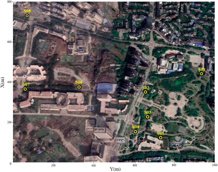
FIGURE 1. Location map of the dense array.
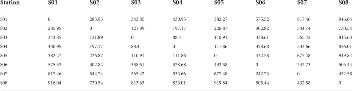
TABLE 1. Separation distance of station-to-station (unit: m).
TABLE 2. Parameters of strong motion recordings.
To accurately quantify the amplitude level of acceleration time history, the root mean square acceleration
where Td=T1-T2 represents the relative duration of ground motion. In this paper, the S-bands of the earthquake events in Luxian and Yibin are the main research objects; thus, T1 and T2 are the start and end times, respectively, of the S-waves in the observation records. Before starting the calculation, the following processes must be carried out for the two sets of observation records. 1) Subtract the average value of noise 10 s before the event from the original data to return the observed waveform to zero (Boore, 2001). 2) Perform bandpass filtering in the range of 0.05–50 Hz on the data using the fourth-order Butterworth filter to eliminate the influence of environmental factors and instrument self-noise on the acceleration time history. 3) Eliminate the first arrival time fluctuations caused by the wave passage effect using the waveform cross-correlation method, and align the waveform (Boissières and Vanmarcke, 1995). The S-wave time window is intercepted as shown in Figure 2:
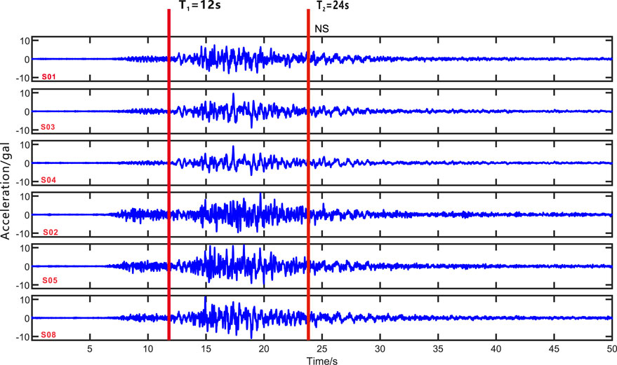
FIGURE 2. Schematic diagram of time window interception (NS component of the Luxian earthquake).
For the Luxian earthquake, the time windows of each component are set to the range of 12–24 s, which covers the whole period from the first arrival of shear waves to the maximum energy, thereby effectively avoiding the interference of a signal singular value on peak ground acceleration (PGA). The window selection principle of the Yibin earthquake records is the same as that of the Luxian earthquake, with a time truncation of 20–32 s, and the relative duration is 12 s. The slight difference in the S-wave delay caused by different source parameters does not affect the final calculation result. The calculation results of the RMS acceleration are shown in Figure 3.
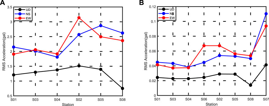
FIGURE 3. Spatial distribution of root-mean-square acceleration: (A) RMS acceleration of the Luxian earthquake; (B) RMS acceleration of the Yibin earthquake.
Comparing the earthquake events,
The acceleration Fourier spectra are shown in Figure 4, which are divided into two groups, one for each earthquake event. The amplitude spectrum curve is smoothed using the Konno–Ohmachi algorithm (the smoothing coefficient is 50) so as to suppress random disturbances (Konno and Ohmachi, 1998). For the same observation station, affected by the magnitude and epicenter distance, the Fourier spectrum of the Luxian earthquake (Figure 4A) is several tens of times higher than that of the Yibin earthquake (Figure 4B), and its effective frequency signal band is 0.05–20 Hz, slightly wider than that of the Yibin earthquake. The following trends can also be seen in the figure.
1) In Figure 4A (the Luxian earthquake), the amplitude spectra of the three-component record at each station are in high consistency below 5 Hz (except S08), but spectra of S02 and S05 are amplified compared with those of S01, S03, and S04 when the frequency exceeds 5 Hz. This amplification is particularly obvious in the horizontal component. The amplitude spectrum of S08 in the vertical component is lower than that of the other stations below 5 Hz, but the low-frequency part is consistent with that of the other stations in the horizontal component, indicating that site conditions at this point are distinctive. The amplitude spectrum of this point is also amplified to different degrees in the two horizontal components, and the affected frequency band is wider than that of S02 and S05.
2) In Figure 4B (the Yibin earthquake), the spatial variation characteristics of the spectra in common stations resemble the observation results of the Luxian earthquake. The frequency-domain amplification of S07 is most obvious, starting at 2.5 Hz, and the corresponding root mean square acceleration shown in Figure 3B is also the greatest.
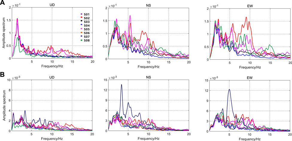
FIGURE 4. Acceleration amplitude spectra of different observation points: (A) amplitude spectra of the Luxian earthquake and (B) amplitude spectra of the Yibin earthquake.
The observation results show that the energy of the two groups of the acceleration time histories is limited, but its characteristics of spatial variation are obvious. In addition, the amplitude–frequency difference of the horizontal component is much larger than that of the vertical component, which is mainly reflected in the frequency domain above 2.5 Hz. The heterogeneity of the site soil layer is the fundamental cause of the aforementioned changes, and this will be studied and discussed in the following section.
The array is located in the southern limb of the Ziliujing Anticline, where the site is relatively flat and free of large faults; therefore, the geological structure is simple. The exposed soil of the site mainly includes the Quaternary Holocene backfill (backfill time is 7–20 years) and residual slope clay, and the estimated shear wave velocity is close to 200 m/s. The influence of this soil layer on ground motion is mainly manifested as an amplification effect therefore, the horizontal-to-vertical spectrum ratio (H/V) can be calculated to distinguish site types in the absence of borehole data. In this section, this method is adopted to simultaneously analyze the microtremor and acceleration records and then evaluate the heterogeneity of the soil layer from the perspectives of predominant frequency and amplification.
The three-component microtremor data are selected from the continuous waveform recorded using the instrument at night (after 22:00). Next, the anti-STA/LTA algorithm is used to eliminate short-time interference, and a period of 30 min is intercepted to calculate the spectrum ratio according to Eq. 2:
where
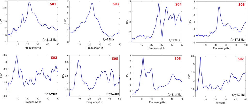
FIGURE 5. Microtremor H/V ratios of each soil station.
Many studies have shown that the predominant frequency of the H/V spectral ratio is nearly close to the resonant frequency of the sedimentary layer, which has a negative exponential relation with the depth of the soil–rock interface. Therefore, the higher the predominant frequency, the smaller the thickness (Ibs-von Seht and Wohlenberg, 1999; Parolai et al., 2002; Dinesh et al., 2010; Rong et al., 2016; Joshi et al., 2018; Peng et al., 2020; Shi and Chen, 2020). In view of this, we can infer that the difference in the overburden thickness is an important factor causing the spatial variation of acceleration amplitude. However, the aforementioned inference cannot explain the low-frequency attenuation of vertical records of S08, which needs to be further analyzed in combination with strong motion acceleration records.
In this section, the horizontal–vertical acceleration response spectrum ratios are used to quantify the amplification effect of the soil layers. The damping ratio of this study is
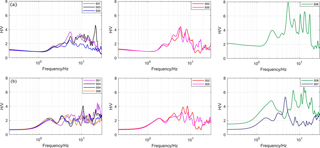
FIGURE 6. Response spectral H/V ratio of each soil station: (A) H/V ratios of the Luxian earthquake and (B) H/V ratios of the Yibin earthquake.
By comparing S01‒S07, the spectrum ratio curves of stations with similar site conditions are also shown to be consistent, such as S01 and S03, and S02 and S05. Additionally, the amplification of the S04 and S06 curves is lower than that of the other soil layer stations, while there is little difference in S01 and S03. The flatness of the response spectrum H/V curves of the seven stations corresponds to the predominant frequency. The higher the predominant frequency, the smaller will be the thickness of the overburden, and the flatter the spectrum ratio curve. The spectral ratio curve of S08 is the most distinctive. For S08, although the estimated soil layer thickness is between S01 and S05, the H/V curve is the steepest, with the highest amplification of 8. It indicates that thickness is not the only factor affecting the amplitude–frequency characteristics of acceleration. Combined with the multipeak characteristics of the curve at this station, it is indicated that S08 has a soft interlayer and tends to be a class III site (Ji, 2014). Considering that there is more noise interference in the case of too little ground motion energy, the amplification effect of the Yibin earthquake is not as obvious as that of the Luxian earthquake. However, after comparing the curve characteristics of the stations, the classification results of the site conditions are consistent (Figure 6B). In addition, the amplification (combined with Figures 4, 5), predominant frequency, and H/V curve characteristics of S07 differ significantly from those of S02 and S05. Although the three stations belong to class II soil layers, in the follow-up study, it is still considered as independent soil conditions.
By analyzing the characteristics of the H/V spectrum ratio, it is inferred that the discrepancy in the overburden thickness leads to the spatial variation in the acceleration amplitude and spectrum. The presence of the soft interlayer increases the complexity and uncertainty of the site effect at S08. It also amplifies the horizontal acceleration and attenuates the vertical acceleration. In conclusion, the properties of the soil contained in the array can be divided into four types, but the specific situation must be determined by subsequent drilling exploration or by referring to strict site classification methods (Wen et al., 2011). This paper mainly aims to study the impact of these differences in soil properties on the spatial variation of ground motion.
The amplification effect of the classification and thickness of the soil layer on the bedrock incident wave will alter the amplitude and spectrum of the ground motion. With the gradual improvement of the theory, our researchers found that the heterogeneity of the site would also change the shape of the lagged coherency curve, and this mechanism was more complex than we had imagined. In view of this, the lagged coherency of different pairs of the stations is calculated based on the existing observation data, and the variation law of strong motion spatial coherency in heterogeneous soil sites is analyzed from a practical perspective.
Assuming that the ground motion is an ergodic stationary random process and the acceleration time histories of points k and l at a distance of d are
where N is the time length of the intercepted shear wave, and
After further derivation,
where
Next, combining Formulas (5), (6) and (7), the cross-power spectral density is normalized to obtain the coherency function expression:
The absolute value of the coherency function is between 0 and 1, representing the correlation of different frequency components of multipoint ground motions. In engineering practice, this is called lagged coherency and is regarded as an important index to measure the spatial variation of strong ground motions. The imaginary part
The spectrum obtained by the traditional Fourier transform will contain much spike interference, causing the lagged coherency to remain constant at 1 throughout the frequency band. In this regard, the power spectral density is smoothed by referring to the multiorder Slepian window proposed by Thomeson (1982), and the result is obtained by weighted summation. The specific implementation steps are shown in Supplementary Appendix S1. Compared with the single-window smoothing power spectrum estimation method, the multiwindow spectrum analysis has a small deviation and variance, and the result is closer to the real spectrum.
The lagged coherency curved surface between different pairs of stations is estimated based on the multiwindow spectrum theory, as shown in Figure 7. The variation amplitude of the coherency function with frequency is greater than that with spatial distance, and there are several rules. First, with the increase of frequency, the values of the lagged coherency first rapidly decay and then fluctuate slightly, exhibiting multipeak characteristics in the middle- and high-frequency band (5–20 Hz). The variation laws of different vibration directions also differ. The vertical component decays faster with frequency, and the peak jitter of the high-frequency part is not as obvious as that of the horizontal component. Meanwhile, the coherency of the EW and NS components has a trend similar to that of the frequency. As shown by the comparison result of the two groups of calculations, overall, the lagged coherency of the Yibin earthquake is higher than that of the Luxian earthquake. Since there are many station pairs, the stereogram is clearer.
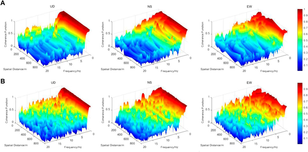
FIGURE 7. Lagged coherency 3D stereogram: (A) stereogram of the Luxian earthquake and (B) stereogram of the Yibin earthquake.
The comparison of the lagged coherency curves of station pairs is shown in Figure 8, arranged from small to large spatial distance. It is observed that the coherency function curve of the vertical component first decays with the frequency, shows the first “valley” at 3‒7 Hz, and then increases slightly and decays in an oscillatory manner. This “valley” is called a “coherency hole” in the work of Zerva, and the corresponding frequency is the average of the predominant frequency (f0) of the whole heterogeneous soil site (Zerva and Harada, 1997). However, this concept does not apply here because f0 of most sites exceeds 8 Hz and falls within this range only in S07. Therefore, the theoretical model has certain limitations, and this paper instead refers to it as the “frequency inflection point.” Compared with the vertical component, the “inflection points” in the two horizontal directions are slightly blurred, and the oscillation amplitude of the curve at a high frequency is greater.
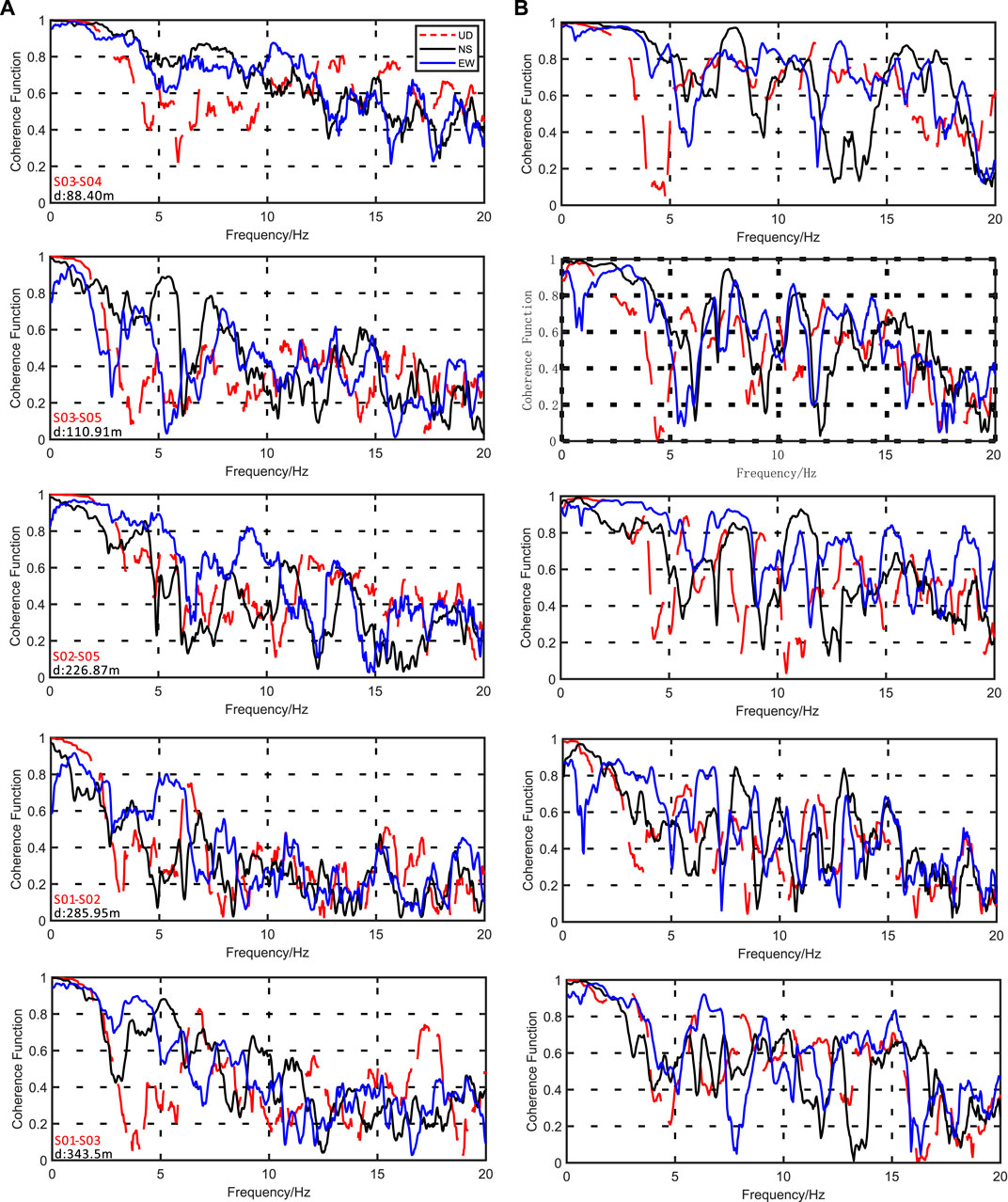
FIGURE 8. Variation in lagged coherency as functions of frequency: (A) coherency curves of the Luxian earthquake and (B) coherency curves of the Yibin earthquake.
The local soil conditions are obviously correlated with the lagged coherency between stations. First, the records of the Luxian earthquake are analyzed (Figure 8A). The separation distance between S03 and S04 is about 88.4 m, and the three components show the highest correlation as a whole, while the lagged coherency of their horizontal components remains around 0.8 even in the middle frequency band (5–12 Hz). The predominant frequency and flatness of the corresponding H/V curves of the two stations are also similar (Figures 5, 6). The site effects of the station pair S02–S05 are basically the same, and the coherency of the whole frequency band is significantly higher than that of S02–S01. Similarly, the coherency of S03–S01 is also greater than that of S02–S01 with slightly smaller station spacing, indicating that the difference in soil conditions will cause coherency loss. However, this is not the only factor affecting the coherency function, since the station-to-station distance also plays a role.
Compared with S03–S05, the horizontal component of S02–S05 does not exhibit obvious site advantages. The reason for this is that the latter has a larger distance than the former, with a difference of more than 100 m. Although the response spectrum H/V curves of S03 and S01 are in the highest agreement (Figure 6), the separation distance d exceeds 300 m, and the coherency function is generally (f>5) lower than those of S03–S04 and S03–S05. The analysis results show that the station spacing d and site conditions jointly affect the coherency of soil ground motions. However, when d does not differ much, the site conditions have a greater impact on the coherency function, and this influence mechanism is also quite obvious in the calculation results of the vertical direction.
After observing the corresponding calculation results of the Yibin earthquake (Figure 8B), almost the same conclusion can be drawn, even though the coherency loss in the horizontal direction caused by heterogeneous site conditions is not as obvious as that of the Luxian earthquake.
To avoid the subjectivity of artificially selecting coherency samples, all lagged coherency curves are summed and averaged according to the four frequency bands of 0.1–5, 5–10, 10–15, and 15–20 Hz (representing low, medium, medium-high, and high frequency, respectively). Then, the scatter plots of the coherency function change with station spacing d at different scales are drawn. According to the discussion results in Section 3, the asterisk “*” represents the station pairs of the same site type (including the station pairs between S01, S03, S04 and S06, and S02-S05), and the circle “○” represents the station pairs between other different site types. Figures 9, 10 show the two sets of scatter points. All of the scatter points of the lagged coherency attenuate with the increase in the separation distance d and decrease with the increase of the frequency. Specifically, the values of the vertical component decrease faster with the frequency, and the attenuation trend of the mid-high-frequency band (5–20 Hz) with the distance is blurred compared with the horizontal component. Comparing different types of scatter distribution, the two earthquake events show similar characteristics. In other words, the scatter-lagged coherency distribution of the station pair with the same soil conditions is more concentrated, and the value is higher. Due to the uncertainty of the spatial variation of ground motion, it is also observed that the coherency coefficient of some “○” scatter points is larger than that of “*” scatter points with equal (or even smaller) station spacing, but the high coherency brought by site consistency is a common phenomenon.
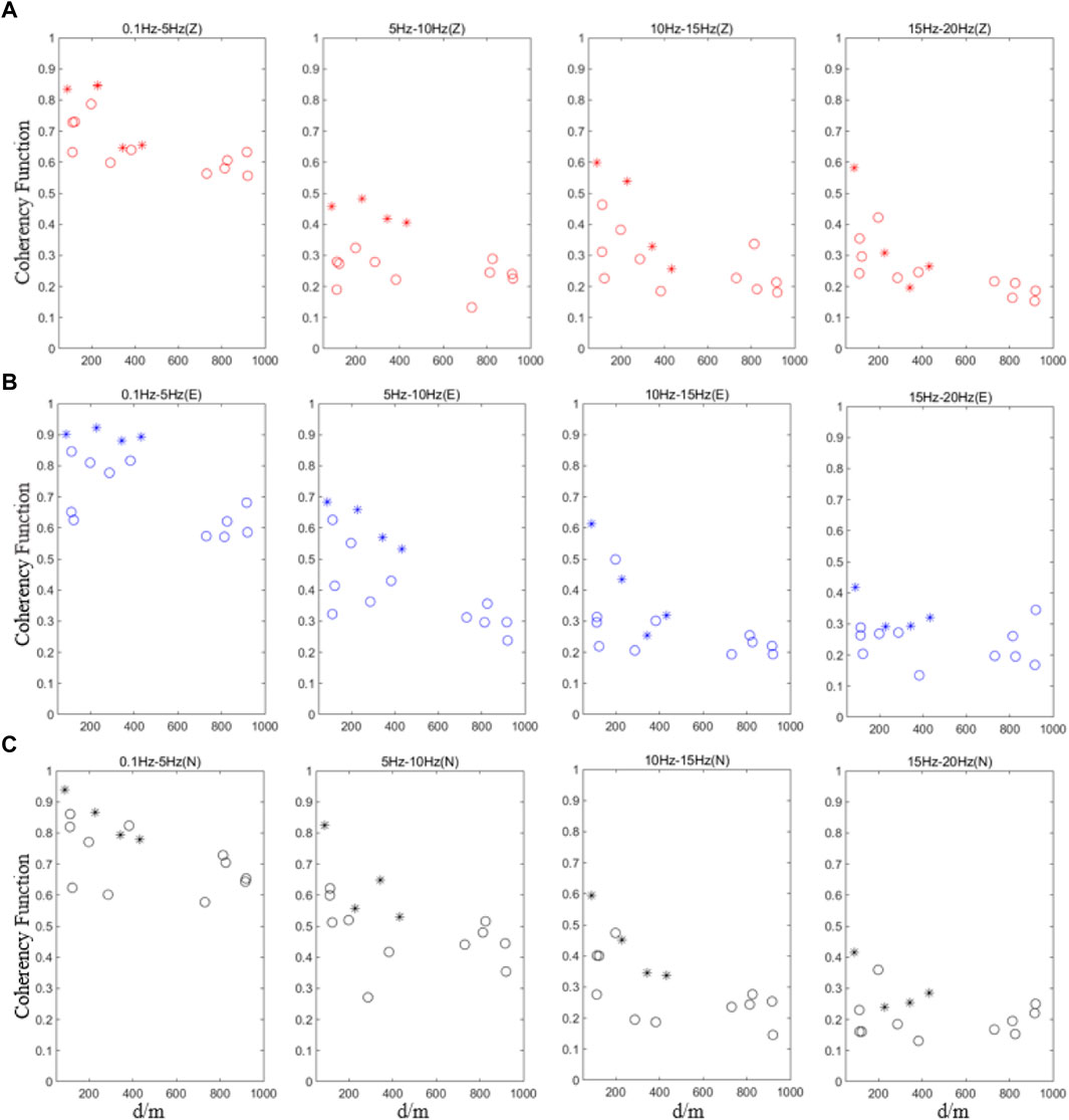
FIGURE 9. Variation in lagged coherency as functions of distance (the Luxian earthquake). The asterisk (*) represents the station pairs of the same site type, and the circle (○) represents the station pairs between other different site types. (A) UD component, (B) EW component, and (C) NS component.
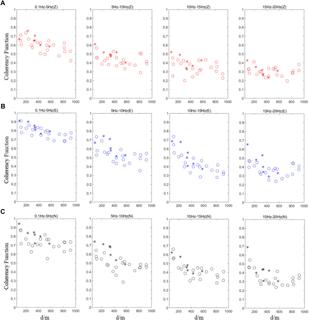
FIGURE 10. Variation in lagged coherency as functions of distance (the Yibin earthquake). The asterisk (*) represents the station pairs of the same site type, and the circle () represents the station pairs between other different site types. (A) UD component, (B) EW component, and (C) NS component.
In summary, the heterogeneity of the soil layer will also bear an impact on the lagged coherency. In the case of little difference in the separation distance, the station pairs with similar soil conditions tend to have higher coherency. Different soil conditions will not only reduce the coherency between two points but also make the distribution of coherency more discrete in the spatial domain. Thus, the influence mechanism will not change the general attenuation of coherency with frequency and distance because the influence of the propagation path (incoherency effect) must not be ignored (Abrahamson et al., 1991; Zerva, 2009).
Mathematical modeling is a key step in applying theoretical research to engineering practice. Researchers have established a variety of lagged coherency models according to seismological methods and observation results and then regressed corresponding parameters through observation data to further guide multipoint ground motion input. The coherency loss caused by site heterogeneity has been confirmed in the previous section of this paper, but this change mechanism cannot be directly explained by the transfer function of a soil seismic response, since lagged coherency is the standardization of cross-power spectrum amplitude, and the transfer function will be canceled out in the calculation process. Some scholars have derived the expression of the coherency function in the heterogeneous soil site through the response spectrum theory. However, it is also a macro-model given under the assumption that the soil characteristics are randomly distributed and thus cannot explain the observation results in this study. The results of this study agree with Kiureghian’s view that the coherency loss caused by the heterogeneity of the soil layer is also attributed to the incoherency effect, ignoring the influence of the medium attenuation and finite source (Somerville et al., 1988). The lagged coherency function can be expressed in the following form:
where
where
In Yu’s study, the cut-off frequency
where parameters
The model is controlled by three variables, that is, frequency (f), separation distance (d), and site impact factor (
In order to verify the reliability of the proposed model, Eq. 11 is used to perform nonlinear fitting on the two sets of observation records. The Loh model (Loh and Lin, 1990) and Harichandran–Vanmarcke model (1986, “ H-V ”for short), which are widely used in earthquake engineering today, are selected as references for fitting results in different frequency bands; corresponding empirical formulas are shown in Table 3. Considering that the coherency functions of the NS and EW components are close, the samples of the two are pooled. In the calculation, the frequency increment is df=0.1 Hz, and the lagged coherency curve shown in Figure 9 is fitted according to four frequency bands of 0.1–5, 5–10, 10–15, and 15–20 Hz to ensure the accuracy of results.
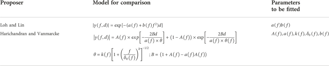
TABLE 3. Empirical lagged coherency model for comparison (according to the research content in this section, the model expression had been slightly modified).
Figures 11, 12 show the comparison of the arithmetic mean value between fitting curves and the mean coherency observed from two events. The solid lines in red and green represent the coherency coefficients of this proposed model when
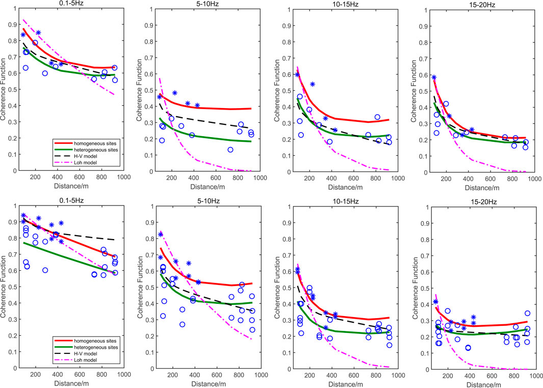
FIGURE 11. Fitting results for the Luxian earthquake: (A) vertical direction and (B) horizontal direction.
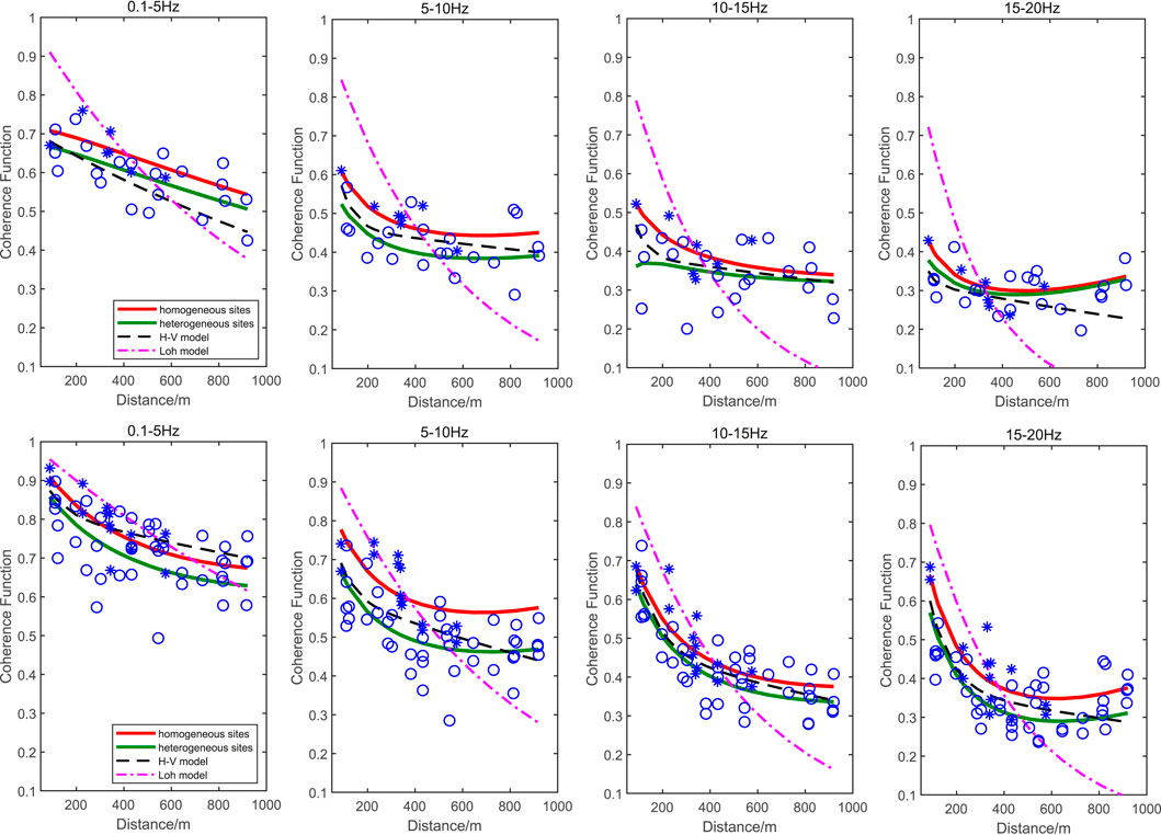
FIGURE 12. Fitting results for the Yibin earthquake: (A) vertical direction and (B) horizontal direction.
Residual analysis was carried out on the fitting results, and the root mean square error (RMSE) was selected as the accuracy evaluation criteria:
where
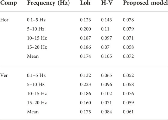
TABLE 4. RMSE of different models’ fitting results for the Luxian Earthquake.
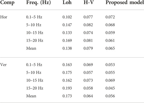
TABLE 5. RMSE of different models’ fitting results for the Yibin Earthquake.
The Loh model has the worst fitting performance, and the fitting RMSE in some frequency bands exceeds 0.2 (Table 4, 5-10 Hz); the RMSE of the H-V model is generally lower than that of the Loh model but higher than our proposed model in each bands. Comparing the mean RMSE, we can find that the residuals of three fitting models for the Luxian earthquake are higher than those of the Yibin earthquake due to smaller sample size and more discrete distribution of lagged coherency. However, our model takes into account the effect of site heterogeneity, and the fitting RMSE could be controlled below 0.08 in each frequency band.
Practical application shows that the ideal simulation results throughout the frequency range can be obtained with the soil-heterogeneity lagged coherency model developed in this study.
Based on observation records of the Luxian MS 6.0 earthquake and Yibin MS 5.1 earthquake obtained using the Zigong dense array, we first studied the spatial variability of strong motion in heterogeneous soil from a practical perspective. Multiple technical methods are then comprehensively utilized to quantify the amplification effects and classify the site conditions in the study. On this basis, the lagged coherency of different station pairs was analyzed, and the impact of local soil conditions on the lagged coherency was emphatically discussed, which led to a fascinating new insight. Finally, a coherency function model considering the influence of a heterogeneous soil site is constructed using a mathematical method, and the nonlinear fitting results are compared with two traditional empirical models. The following conclusions can be drawn from this study:
1) The amplitude characteristics of ground motion change with the spatial position attributed to local soil conditions, and the affected frequency bands also differ. The root-mean-square acceleration of most stations increases with the decrease of the dominant frequency, and the horizontal component is much more affected than the vertical component. The H/V spectrum ratio method can be used to clearly show the site effect of each station, making site classification, and assist in studying the spatial variation of strong ground motion.
2) As shown by the calculation results of lagged coherency, the correlation between stations decreases with frequency and separation distance. However, the heterogeneity of the soil layer interferes with this change trend. The station pairs with similar H/V spectrum ratio characteristics have higher coherency and may be larger than those with smaller distance. When the site conditions differ greatly, the coherency is greatly reduced, thus making the scatter distribution more discrete. This effect is also quite obvious in the low-frequency part below 5 Hz. Comparing the calculation results of the two groups of observation data of the Luxian MS 6.0 earthquake and Yibin MS 5.1 earthquake, the conclusion is consistent.
3) Considering that the bedrock incident wave may be affected by additional incoherency effects when passing through the heterogeneous soil layer, a novel coherency function model is established. The proposed model was controlled by three variables, namely, frequency, interstation distance, and site impact factor, and the lagged coherency attenuation trend of different station pairs can be simulated through a set of parameters. In addition, its fitting precision was obviously better than that of the Loh model and H-V model which are popular in engineering at present.
In this study, the influence of soil heterogeneity on the spatial variation of ground motion could not be ignored. The previous lagged coherency models obtained based on the dense array are all in accordance with the soil homogeneous assumption, which could not reflect the change in the coherency coefficient by local site factors. The new model proposed in this paper could make up for such shortcomings to some extent and is an advance in research methods. For middle- and far-field earthquakes (R>50 km), the spatial coherence of observation records is mainly affected by the propagation path and site conditions (incoherent effect). The source finiteness contributes little to the coherency loss (Huda and Langston, 2021; Abbas and Tezcan 2020). Consequently, the conclusions and model summarized in this paper are also of high reference value and at least provide good lower-bound estimates of the spatial incoherence of larger magnitude earthquakes for earthquake fortification. However, this proposed model cannot distinguish soil heterogeneity in detail due to the limited observation data. Therefore, it is needed to collect more strong motion records of dense arrays and borehole data in heterogeneous soil sites, optimize the classification of the heterogeneous soil layer, and achieve better application results (Supplementary Appendix S1).
The raw data supporting the conclusions of this article will be made available by the authors, without undue reservation.
QY: data analysis, numerical calculation and model building, and writing of manuscript with RY; RY: daily advisor, conception and design of the study, and writing of manuscript with QY; PJ: operation and maintenance of the array, data reception, and data preprocessing; and KC: providing codes for response spectrum calculation and drawing H/V spectral ratio curves with QY.
This study is supported by the Natural Science Foundation of China (No. 51878627) and the Special Foundation of Geophysics, China Earthquake Administration (No. DQJB 21B36).
The authors declare that the research was conducted in the absence of any commercial or financial relationships that could be construed as a potential conflict of interest.
All claims expressed in this article are solely those of the authors and do not necessarily represent those of their affiliated organizations, or those of the publisher, the editors, and the reviewers. Any product that may be evaluated in this article, or claim that may be made by its manufacturer, is not guaranteed or endorsed by the publisher.
The Supplementary Material for this article can be found online at: https://www.frontiersin.org/articles/10.3389/feart.2022.1054448/full#supplementary-material
Abbas, H., and Tezcan, J. (2006). Analysis and modeling of ground motion coherency at uniform site conditions. Soil Dynamics and Earthquake Engineering 133, 106124. doi:10.1016/j.soildyn.2020
Abrahamson, N. A., Schneider, J. F., and Stepp, J. C . (1991). Empirical spatial coherency functions for application to soil-structure interaction analyses. Earthq. Spectra 7 (1), 1–27. doi:10.1193/1.1585610
Abrahamson, N. A., Bolt, B. A., Darragh, R. B., Penzien, J., and Tsai, Y. B. (1987). The smart I accelerograph array (1980-1987): A review. Earthq. Spectra 3, 263–287. doi:10.1193/1.1585428
Bi, K. M., and Hao, H. (2012). Influence of ground motion spatial variations and local soil conditions on the seismic responses of buried segmented pipelines. Struct. Eng. Mech. 44 (5), 663–680. doi:10.12989/sem.2012.44.5.663
Boissières, H., and Vanmarcke, E. H. (1995). Spatial correlation of earthquake ground motion: Non-parametric estimation. Soil Dyn. Earthq. Eng. 14 (1), 23–31. doi:10.1016/0267-7261(94)00027-e
Boore, D. M. (2001). Effect of baseline corrections on displacements and response spectra for several recordings of the 1999 chi-chi, taiwan, earthquake. Bull. Seismol. Soc. Am. 91 (5), 1199–1211. doi:10.1785/0120000703
Chen, Y., Bradley, B. A., and Baker, J. W. (2021). Nonstationary spatial correlation in New Zealand strong ground-motion data. Earthq. Eng. Struct. Dyn. 50 (13), 3421–3440. doi:10.1002/eqe.3516
Chern, C. C. (1982). “Preliminary report on the smart 1 strong motion array in taiwan,” in Earthquake engineering research center report No. UCB/EERC-82/13 (Berkeley CA: Univ of California).
Cornou, C., Bard, P-Y., and Dietrich, M. (2003). Contribution of dense array analysis to the identification and quantification of basin-edge-induced waves, Part II: Application to grenoble basin (French alps). Bull. Seismol. Soc. Am. 93, 2624–2648. doi:10.1785/0120020140
Dinesh, B. V., Nair, G. J., Prasad, A. G. V., Nakkeeran, P., and Radhakrishna, M. (2010). Estimation of sedimentary layer shear wave velocity using micro-tremor H/V ratio measurements for Bangalore city. Soil Dyn. Earthq. Eng. 30 (11), 1377–1382. doi:10.1016/j.soildyn.2010.06.012
Goda, K., and Hong, H. P. (2008). Spatial correlation of peak ground motions and response spectra. Bull. Seismol. Soc. Am. 98 (1), 354–365. doi:10.1785/0120070078
Hao, H., Oliveira, C. S., and Penzien, J. (1989). Multiple-station ground motion processing and simulation based on smart-1 array data. Nucl. Eng. Des. 111 (3), 293–310. doi:10.1016/0029-5493(89)90241-0
Harichandran, R. S., and Vanmarcke, E. H. (1986). Stochastic variation of earthquake ground motion in space and time. J. Eng. Mech. 112 (2), 154–174. doi:10.1061/(asce)0733-9399(1986)112:2(154)
Huda, M. M., and Langston, C. A. (2021). Coherence and variability of ground motion in New Madrid Seismic Zone using an array of 600 m. J. Seismol. 25 (2), 433–448. doi:10.1007/s10950-020-09970-z
Ibs-von Seht, M., and Wohlenberg, J. (1999). Microtremor measurements used to map thickness of soft sediments. Bull. Seismol. Soc. Am. 89 (1), 250–259. doi:10.1785/bssa0890010250
Imtiaz, A., Cornou, C., Bard, P. Y., and Zerva, A. (2018). Effects of site geometry on short-distance spatial coherency in Argostoli, Greece. Bull. Earthq. Eng. 16 (5), 1801–1827. doi:10.1007/s10518-017-0270-z
Ji, K. (2014). Estimation on site characteristic based on H/V spectral ratio method[D]. Harbin: Institute of Engineering Mechanics, CEA.
Joshi, A. U., Sant, D. A., Parvez, I. A., Rangarajan, G., Limaye, M. A., Mukherjee, S., et al. (2018). Subsurface profiling of granite pluton using microtremor method: Southern Aravalli, Gujarat, India. Int. J. Earth Sci. 107 (1), 191–201. doi:10.1007/s00531-017-1482-9
Katayama, T. (1991). Use of dense array data in the determination of engineering properties of strong motions. Struct. Saf. 10, 27–51. doi:10.1016/0167-4730(91)90005-t
Kiureghian, A. D. (1996). A coherency model for spatially varying ground motions. Earthq. Eng. Struct. Dyn. 25 (1), 99–111. doi:10.1002/(sici)1096-9845(199601)25:1<99::aid-eqe540>3.0.co;2-c
Konakli, K., Der Kiureghian, A., and Dreger, D. (2014). Coherency analysis of accelerograms recorded by the UPSAR array during the 2004 Parkfield earthquake. Earthq. Eng. Struct. Dyn. 43 (5), 641–659. doi:10.1002/eqe.2362
Konno, K., and Ohmachi, T. (1998). Ground-motion characteristics estimated from spectral ratio between horizontal and vertical components of microtremor. Bull. Seismol. Soc. Am. 88 (1), 228–241. doi:10.1785/bssa0880010228
Kwok, A. O. L., Stewart, J. P., and Hashash, Y. M. A. (2008). Nonlinear ground-response analysis of Turkey flat shallow stiff-soil site to strong ground motion. Bull. Seismol. Soc. Am. 98 (1), 331–343. doi:10.1785/0120070009
Laib, A., Laouami, N., and Slimani, A. (2015). Modeling of soil heterogeneity and its effects on seismic response of multi-support structures. Earthq. Eng. Eng. Vib. 14 (3), 423–437. doi:10.1007/s11803-015-0034-1
Liao, S., and Li, J. (2002). A stochastic approach to site-response component in seismic ground motion coherency model. Soil Dyn. Earthq. Eng. 22, 813–820. doi:10.1016/s0267-7261(02)00103-3
Loh, C. H., and Lin, S. G. (1990). Directionality and simulation in spatial variation of seismic waves. Eng. Struct. 12 (2), 134–143. doi:10.1016/0141-0296(90)90019-o
Loh, C. H., Penajien, J., and Tsai, Y. B. (1982). Engineering analysis of smart-1 seismic data. Int. J. Earthq. engineering\&\structural Dyn. 10, 575–591.
Loh, C. H., and Yeh, Y. T. (1988). Spatial variation and stochastic modelling of seismic differential ground movement. Earthq. Eng. Struct. Dyn. 16 (4), 583–596. doi:10.1002/eqe.4290160409
Nakamura, Y., and Saito, A. (1983). “Estimations of amplification characteristics of surface ground and PGA using strong motion records (in Japanese) [C],” in Proceeding of the 17th JSCE Earthquake Eng. Symp, 25–28.
Nechtschein, S., Ba, Rd P. Y., Gariel, J. C., Meneroud, J. P., Dervin, P., Gaubert, C., et al. (1996). “A topographic effect study in the Nice region[C],” in Proceeding of the International conference on seismic zonation, Jaunary 1996.
Nour, A., Slimani, A., Laouami, N., and Afra, H. (2003). Finite element model for the probabilistic seismic response of heterogeneous soil profile. Soil Dyn. Earthq. Eng. 23 (5), 331–348. doi:10.1016/s0267-7261(03)00036-8
O' Rourke, M. J., Castro, G., and Centola, N. (1980). Effects of seismic wave propagation upon buried pipelines. Earthq. Eng. Struct. Dyn. 8 (5), 455–467. doi:10.1002/eqe.4290080507
Parolai, S., Bormann, P., and Milkereit, C. (2002). New relationships between VS, thickness of sediments, and resonance frequency calculated by the H/V ratio of seismic noise for the Cologne Area (Germany). Bull. Seismol. Soc. Am. 92 (6), 2521–2527. doi:10.1785/0120010248
Peng, F., Wang, W. J., and Kou, H. D. (2020). Microtremer H/V spectral ratio investigation in the sanhe-pinggu area: Site responses, shallow sedimentary structure, and fault activity revealed. Chin. J. Geophys 63 (10), 3775–3790. (in Chinese). doi:10.6038/cjg2020O0025
Rong, M. S., Li, X. J., Wang, Z. M., Lv, Y. Z., et al. (2016). Applicability of HVSR in analysis of site-effects caused by earthquakes. Chin. J. Geophys 59 (8), 2878–2891. (in Chinese). doi:10.6038/cjg2018L0171
Rosalba, M., Lucia, N., Terenzio, G. F., and Potenza, M. R. (2018). Ambient noise HVSR measurements in the Avellino historical centre and surrounding area (southern Italy). Correlation with surface geology and damage caused by the 1980 Irpinia-Basilicata earthquake. Measurement 130, 211–222. doi:10.1016/j.measurement.2018.08.015
Sadouki, A., Harichane, Z., and Chehat, A. (2012). Response of a randomly inhomogeneous layered media to harmonic excitations. Soil Dyn. Earthq. Eng. 36, 84–95. doi:10.1016/j.soildyn.2012.01.007
Schneider, J. F., Stepp, J. C., and Abrahamson, N. A. (1992). “The spatial variation of earthquake ground motion and effects of local site” in Proc. Earthquake Engng. 10th World Conf. Madrid, Spain, 967–972
Shi, L. J., and Chen, S. Y. (2020). The applicability of site characteristic parameters measurement based on micro-tremor’s H/V spectra. J. Vib. Shock 39 (11), 138–145. doi:10.13465/j.cnki.jvs.2020.11.018
Shi, L. J., Liu, J. X., and Chen, S. Y. (2022). Site classification based on predominant period of microtremor ’s H/V spectral ratio. J. Vib. Shock 41 (13), 34–42. doi:10.13465/j.cnki.jvs.2022.13.00
Somerville, P. G., McLaren, J. P., Saikia, C. K., and Helmberger, D. V. (1988). Site-specific estimation of spatial incoherence of strong ground motion. Geotech. Spec. Publ., 188–202.
Svay, A., Perron, V., Imtiaz, A., Zentner, I., Cottereau, R., Bard, P., et al. (2017). Spatial coherency analysis of seismic ground motions from a rock site dense array implemented during the Kefalonia 2014 aftershock sequence. Earthq. Eng. Struct. Dyn. 46 (12), 1895–1917. doi:10.1002/eqe.2881
Thomeson, D. J. (1982). Spectrum estimation and harmonic analysis. Proc. IEEE 70 (9), 1055–1096. doi:10.1109/proc.1982.12433
Wang, H. Y., and Xie, L. L . (2010). Effects of topography on ground motion in the xishan park, zigong city. Chin. J. Geophys. 53 (7), 1631–1638. doi:10.3969/j.issn.0001-5733.2010.07.014
Wang, Z. Z. (2012). Coherence variation of ground motion with depths[D]. Dalian: Dalian University of Technology.
Wen, R., Ren, Y., and Shi, D. (2011). Improved HVSR site classification method for free-field strong motion stations validated with Wenchuan aftershock recordings. Earthq. Eng. Eng. Vib. 10 (3), 325–337. doi:10.1007/s11803-011-0069-x
Yang, Q. M. (2008). The divisional evaluation of urban environmental geology in Zigong City[M]. Chendu: Chengdu University of Technology.
Yu, R. F., Abduwaris, A., and Yu, Y. X. (2020). Practical coherency model suitable for near- and far-field earthquakes based on the effect of source-to-site distance on spatial variations in ground motions. Struct. Eng. Mech. 73 (6), 651–666. doi:10.12989/sem.2020.73.6.651
Yu, R. F., Wang, S. Q., and Yu, Y. X. (2021). Reviewing of stochastic description of the spatial variation of ground motion and coherence function model. Rev. Geophys. Planet. Phys. 52 (2), 194–204. doi:10.19975/j.dqyxx.2020-012
Zerva, A. (2009). Spatial variation of seismic ground motion[M]. Boca Raton: CRS Press, Talor and Francis Group.
Zerva, A., and Stephenson, W. R. (2011). Stochastic characteristics of seismic excitations at a non-uniform (rock and soil) site. Soil Dyn. Earthq. Eng. 31, 1261–1284. doi:10.1016/j.soildyn.2011.05.006
Zerva, A., and Zhang, O. (1997). Correlation patterns in characteristics of spatially variable seismic ground motions. Earthq. Eng. Struct. Dyn. 26 (1), 19–39. doi:10.1002/(sici)1096-9845(199701)26:1<19::aid-eqe620>3.0.co;2-f
Zerva, A., and Harada, T. (1997). Effect of surface layer stochasticity on seismic ground motion coherence and strain estimates. Soil Dyn. Earthq. Eng. 16 (7-8), 445–457. doi:10.1016/s0267-7261(97)00019-5
Keywords: heterogeneous soil site, dense array, spatial variation of ground motion, H/V spectral ratio method, lagged coherency
Citation: Yang Q, Yu R, Jiang P and Chen K (2023) Spatial variation of strong ground motions in a heterogeneous soil site based on observation records from a dense array. Front. Earth Sci. 10:1054448. doi: 10.3389/feart.2022.1054448
Received: 26 September 2022; Accepted: 15 November 2022;
Published: 19 January 2023.
Edited by:
Yefei Ren, China Earthquake Administration, Harbin, ChinaReviewed by:
Chaoying Zhao, Chang’an University, ChinaCopyright © 2023 Yang, Yu, Jiang and Chen. This is an open-access article distributed under the terms of the Creative Commons Attribution License (CC BY). The use, distribution or reproduction in other forums is permitted, provided the original author(s) and the copyright owner(s) are credited and that the original publication in this journal is cited, in accordance with accepted academic practice. No use, distribution or reproduction is permitted which does not comply with these terms.
*Correspondence: Ruifang Yu, eXJmYW5nMTI2QDEyNi5jb20=
Disclaimer: All claims expressed in this article are solely those of the authors and do not necessarily represent those of their affiliated organizations, or those of the publisher, the editors and the reviewers. Any product that may be evaluated in this article or claim that may be made by its manufacturer is not guaranteed or endorsed by the publisher.
Research integrity at Frontiers
Learn more about the work of our research integrity team to safeguard the quality of each article we publish.