- TNO, Geological Survey of the Netherlands, Utrecht, Netherlands
A newly developed modelling framework is presented which specifically focusses on the central Oklahoma case and the high-volume injection of wastewater, which led to a surge of induced seismicity. However, the modelling framework is versatile enough to be applied to any anthropogenic subsurface activities and should be seen as a good practice to manage injection while minimizing induced seismicity. The objective is to account for all the available knowledge to deploy the simulation of the flow, induced stress changes and seismicity in the underground. The spatio-temporal pore pressure changes caused by high-volume injection are first determined by using the historical injection rate of the 220 wells at central Oklahoma. From these pressure fields, induced stresses at the basement depth, due to both pore pressure diffusion and poro-elastic inflation of the underground, are computed. The rate-and-state frictional response of the Oklahoma faults is then honored to derive the yearly seismicity rate. After assimilation of the observed seismicity at central Oklahoma, it is demonstrated that our predictions can well explain the historical spatio-temporal evolution of the seismicity at central Oklahoma. Finally, making use of the calibrated predictive model, a constrained optimization approach is used for an efficient screening of multiple injection scenarios. Ultimately, an optimum theoretical scenario is identified which allows the maximization of injection volumes while keeping the seismicity level below a safe cap and, more specifically, would have prevented the dramatical growth of the seismicity rate in 2015. The optimum scenario involves equalizing the injected volumes in all wells and preventing the injection of additional large volumes in the area where most of the wastewater have been already injected prior 2014.
1 Introduction
In response to the rapid increase of the rate of seismicity in 2015 in central and northern Oklahoma, the regulators decided in 2016 to reduce the total volume of injected brine (waste-product of the hydrocarbon industry activities, notably shale gas production) to less than 40% of the 2014 total volume (Ellsworth, 2013; Walsh and Zoback, 2015). Late 2016, large magnitude earthquakes were recorded, and in April 2017 all the wells were shut in. In 2016–2017, the detailed causal relationship between injection operations and seismicity was unclear. In contrast, it is now well recognized and documented that the surge of the number of earthquakes in the central and northern Oklahoma can be attributed to the high-volume injection of brine in the subsurface (Keranen et al., 2014; Weingarten et al., 2015).
Multiple models have already been deployed to study either 1) the physical mechanisms at the origin of the induced events at Oklahoma (Norbeck and Horne, 2016; Goebel et al., 2017a; Goebel et al., 2017b; Johann et al., 2018; Dempsey and Riffault, 2019) or 2) to predict the return of the seismicity increase to a lower background rate after the stop of the injection activities in 2017 (Langenbruch and Zoback, 2016; Goebel et al., 2017a; Goebel et al., 2017b; Langenbruch et al., 2018; Zhai et al., 2019). Up to now, these modelling strategies always involved simplifications either at the level of the simulations of the flow throughout the porous media (Goebel et al., 2017a; Goebel et al., 2017b; Zhai et al., 2019) or at the level of the computations of the induced stress development and seismicity changes (Langenbruch and Zoback, 2016; Norbeck and Horne, 2016; Johann et al., 2018; Langenbruch et al., 2018; Dempsey and Riffault, 2019). In order to gain confidence in the predictive power of any modelling strategy, a thorough model validation against observed data is required. This step has largely been overlooked in existing modelling approaches of induced seismicity at Oklahoma which generally rely on simplified sensitivity analysis.
In this study, a novel modelling approach is outlined that is tailored to honor as much as possible all available pre-existing knowledge at injection sites in the central Oklahoma area (for simplicity the area is simply referred to as “Oklahoma” in the remainder of the manuscript, see Figure 1). Available knowledge consists of data on local geology, flow, mechanical and seismicity response. The model parameters of our seismological model are conditioned with the observed seismicity in order to best fit the full spatio-temporal history of induced earthquakes. It is only after completing this data assimilation procedure that injection strategies can be optimized to maximize the volume of injected brine while minimizing induced seismicity. For optimizing injection strategies, we deployed a constrained optimization workflow that maximizes injection volumes under a fixed limit of allowed seismicity rate. Optimization results show with a different spatio-temporal injection history, the rapid growth of the seismicity rate in 2015 can be successfully prevented while the total volume of injected brine can be maintained. It indicates that injection operations and mitigation measures for induced seismicity greatly benefit from optimization of spatio-temporal injection strategies as seismic risks can be reduced under continuing injection operations.
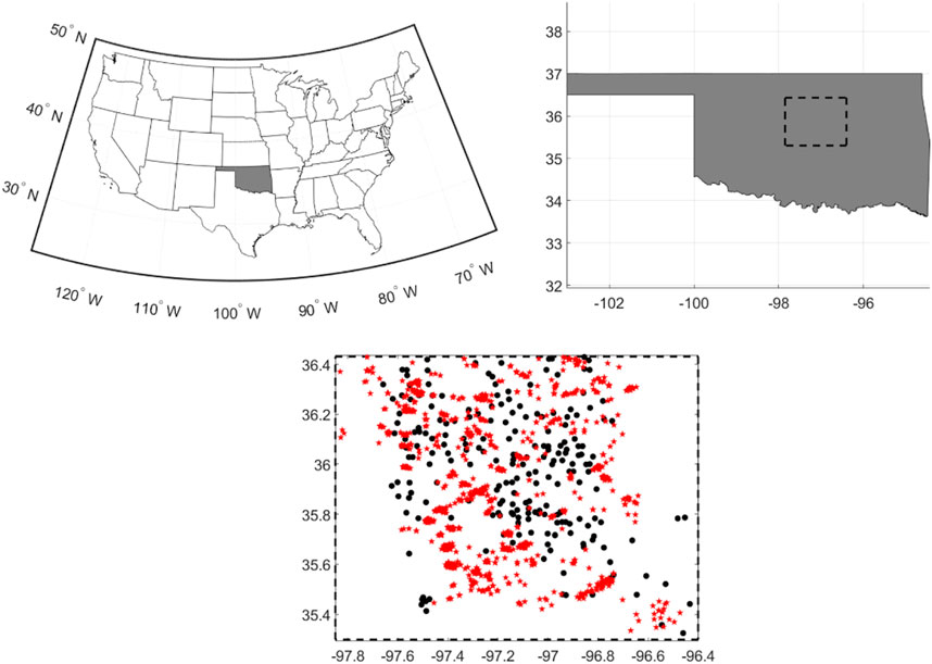
FIGURE 1. Maps of the Oklahoma state in United States showing: (i) the area of interest (dashed contour in top-right map), (ii) the locations of the Arbuckle wastewater disposal wells (black dots in bottom-centre map), (iii) and the Mw3+ earthquakes which nucleated in the basement between 3 and 7 km depth and from 1995 to 2017 (red stars in the bottom-centre map).
2 Methodology
2.1 Flow simulations
The two main identified mechanisms that cause induced seismicity at Oklahoma are: 1) the slow diffusion of elevated pore pressure from the high-permeability Arbuckle aquifer (locus of the brine injections) to its low-permeability basement at the nucleation depth of the induced events (e.g., Langenbruch and Zoback, 2016; Norbeck and Horne, 2016; Dempsey and Riffault, 2019); 2) the change in total stress at this depth in the basement that is caused by poro-elastic loading due to the inflation of the rock volume associated with the increase in pore pressure (e.g., Goebel et al., 2017a; Goebel et al., 2017b; Zhai et al., 2019).
The first modelling effort consists of assessing the historical spatio-temporal distribution of pore pressure changes caused by the high-volume injection of brine in the subsurface at Oklahoma. As in each step of our modelling strategy, this step aims to incorporate all the pre-existing available knowledge on local geology, flow, mechanical and seismicity response at Oklahoma (Johnson, 2008; Faith et al., 2010; Holland, 2013; Keranen et al., 2013; Hincks et al., 2018; Pei et al., 2018). The computation of the pore pressure changes (Figure 2) is performed using the open source OPM-flow simulator (Open Porous Media Initiative, 2020; version 2020.04). OPM-flow is a three-dimensional three-phase fully-implicit reservoir simulator with realistic representation of reservoir geological properties. Wells are incorporated with the standard models used in the commercial simulators from the oil and gas industry. Multiple options are available, as black-oil, thermal, aquifer, CO2; in our specific case we modelled brine. The reader is referred to Rasmussen et al. (2021) for a complete description of OPM-flow.
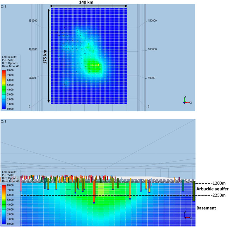
FIGURE 2. Flow simulation—visualization via ResInsight [open source visualization software, ResInsight (Computer Software), version 2020.10, part of Open Porous Media Initiative, Ceentron Solutions, 2020] of the pressure field (changes in pore pressure since the start of injection; in bars) at the end of 2015. Vertical exaggeration x5.
The flow model is populated by properties based on current understanding of the geological and hydrogeological settings at Oklahoma. Three layered-box models have been deployed, each of them including the same thickness for the Arbuckle aquifer and its basement but with different permeabilities and porosities (Table 1). Only the results of the flow simulation with a permeability of 50 and 0.05 mD for the Arbuckle aquifer and its basement, respectively, are discussed in this report (i.e., Model 1 in Table 1). This permeability contrast yields the most likely changes in pressures in the Arbuckle and its basement and is preferred to best match observations.
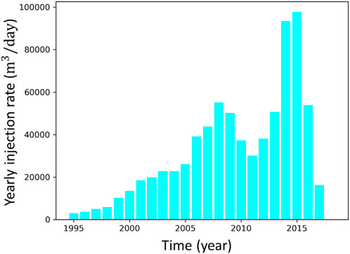
The OPM-FLOW simulation model honors the geographical location and depths of all the wells according to the Oklahoma Corporation Commission. It includes 220 wells for central Oklahoma, the focus area for the present study, and for each of the well injectors the historical monthly injection rate from January 1995 to January 2018 is used as input (Figure 3). Note here that central and western Oklahoma can be considered as isolated and independent compartments in terms of flow (see Zhai et al., 2019); the same modelling complexities are attached to both areas of interest and solely focusing on central Oklahoma is considered sufficient to demonstrate the capabilities of the newly developed modelling framework. The injection depth at the Arbuckle level and distance to the basement is included in our modelling strategy and has been reported as an important parameter correlated with the occurrence of the induced events (Hincks et al., 2018). The run-time of one full OPM-FLOW simulation from January 1995 to January 2018 takes less than 20 min, which is rather fast for such a complex flow simulation. The low computation time makes the simulations suitable for an ensemble-based approach that is used for the optimization. This optimization is the last step of our modelling approach (see Section 2.6).
2.2 Induced stress in the basement
The objective of this modelling step is to assess the spatio-temporal development of induced stresses at the earthquake nucleation depth. Most of the events of the catalog compiled by the Oklahoma Geological Survey are located at a depth between 3 and 7 km (McGarr and Barbour, 2017; Pei et al., 2018). Considering an average depth uncertainty of 2 km, an average earthquake nucleation depth of 4 km depth is considered for our analysis. The two main mechanisms that were identified to control induced stress development and earthquake nucleation at Oklahoma are included: 1) the decrease of the effective normal stress along the basement faults by pore pressure diffusion and 2) the changes in total stresses induced by poro-elastic effects associated with pressure increase and volumetric expansion of rock.
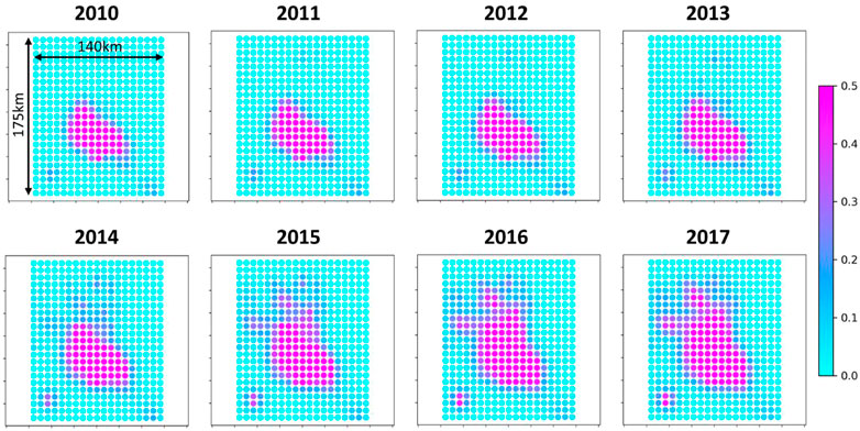
Our modelling approach assumes matrix-dominated flow in the Arbuckle aquifer and fracture-dominated flow in the basement. More specifically highly permeable faults of the basement are assumed to hydraulically connect the base of the porous Arbuckle aquifer to the earthquake nucleation depth. Simple analytical calculations including typical fault properties (diffusivity, porosity, thickness) show that the diffusion time throughout the highly permeable faults-channels is on the order of at most a few days (Zhai et al., 2019). Therefore, one can further assume that the changes in pore pressure modelled by OPM-FLOW at the base of the porous aquifer are representative of the changes in pore pressure at 4 km depth experienced by the basement faults. These changes in pore pressures relatively to the start of injection and along a horizontal plane at 4 km depth are shown in Figure 4. The increase in pore pressure is at first (i.e., 2010) localized at the center of the area of interest and then starts to progressively migrate towards the North-West.
From the spatio-temporal changes in pore pressures at 4 km depth (Figure 4), the changes in the normal effective stress can be directly determined. Analogous to the analysis by Zhai et al. (2019), vertical strike-slip faults with a unique preferred fault strike azimuth of 50° are assumed to be ubiquitous in the basement. This faulting regime and the fault orientation is consistent with the statistical analysis of earthquake focal mechanisms, in situ stress analysis, field mapping, and 3D seismic interpretation at Oklahoma (Holland, 2013; Alt and Zoback, 2016; Kolawole et al., 2019; Qin et al., 2019; Firkins et al., 2020). Principal stresses are assumed to be spatially uniform around Oklahoma with a maximum horizontal stress azimuth oriented at 85°.
Changes in total stress imposed by the volumetric changes of the rock volume is determined using the in-house mechanical simulator MACRIS (Mechanical Analysis of Complex Reservoirs for Induced Seismicity, van Wees et al., 2019; Candela et al., 2019). The main advantage of MACRIS is that it is a mesh-free simulator, i.e., it does not need construction of a dedicated grid for the geomechanical analysis. MACRIS directly takes the grid of the flow simulation as input. In the present case, the grid consists of the 3D pressure fields computed by OPM-FLOW at a yearly sampling rate. Each grid block of the flow simulation is considered as an inflating/compacting nucleus of strain (or center of inflation/compaction, see Mindlin 1936; Geertsma, 1973; Okada, 1992). The contribution of each of these nuclei is integrated to compute the poro-elastic stress change at 4 km depth in the basement. The Barnes-Hut algorithm (Barnes and Hut, 1986) is used for re-discretizing the initial flow grid. The purpose of using this algorithm is twofold: 1) to cluster the nuclei of strain close to the 4 km depth horizontal plane in order to increase the spatial stress resolution, and 2) to shorten the computation time. The approach has been validated by comparison with relatively slow finite-element numerical computations in a previous study (van Wees et al., 2018). The poro-elastic normal and shear stress changes acting on the faults at 4 km depth can thus be calculated using MACRIS. Coulomb stress changes can be evaluated by considering shear stresses and effective normal stresses:
where
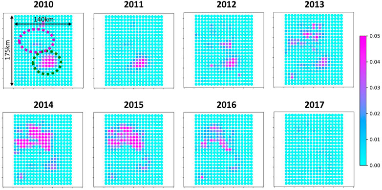
FIGURE 5. Coulomb stress rate fields (in MPa/Year) at 4 km depth along the basement faults. The magenta and green dashed circles in the top-left figure indicates the North area and Central area respectively.
2.3 Induced seismicity
The traditional Coulomb failure model predicts that whenever the Coulomb stress reaches a threshold value, an earthquake is generated (e.g., Ader et al., 2014). Assuming a population of faults on which the pre-stresses are uniformly distributed up to the threshold value, the Coulomb failure model depicts direct proportionality between the seismicity rate and the Coulomb stress rate. For example, during any arbitrary stressing history, the Coulomb failure model predicts an instantaneous reduction or rise of seismic events as soon as the Coulomb stress starts to decrease/increase. This prediction is not in agreement with the observed seismicity in Oklahoma since only a few observed events have been recorded in the year 2009 (cf. Section 2.4). The Coulomb failure model would predict a high seismicity rate that is linearly related to the high Coulomb stress rate in 2010 (Figure 5).
One shortcoming of the Coulomb failure model is that it does not honor the frictional constitutive behavior of faults. Laboratory data show that the timing of dynamic instability of faults depends on initial stress conditions, fault properties and applied stress (Dieterich and Kilgore, 1996). Rate-and-state friction laws have been established in order to reproduce these laboratory observations (see Marone, 1998 for a review). More specifically, the rate-and-state friction laws reproduce the fact that the onset of frictional sliding is a non-instantaneous time-dependent process (as opposed to the instantaneity assumption of the Coulomb model), which introduces a time-dependent failure mechanism for the generation of earthquakes. Now assuming a population of faults following a rate-and-state frictional behavior, and where the time-to-failure of the nucleation spots along the faults is uniformly distributed, Dieterich (1994) derived the following seismicity rate model:
and where
Segall and Lu (2015) reformulated this seismicity rate equation to eliminate the state variable
The differential equation for
where
2.4 Declustering of the observed seismicity
The earthquake catalogue used for our study has been compiled by the Oklahoma Geological Survey. Our analysis is carried on with earthquakes larger or equal to Mw = 3; this minimum magnitude is above the completeness magnitude of the catalogue, and has been selected for sake of comparison with previous studies (e.g., Langenbruch and Zoback, 2016; Zhai et al., 2019). In addition, based on an average depth uncertainty of 2 km and to focus our analysis on the basement only the events nucleating between 3 and 7 km depth are selected. This depth range includes most of the events of the catalog. When this magnitude and depth filtering is applied to the raw earthquake catalogue, the maximum yearly rate of events at Oklahoma reaches roughly 400 events/year in 2015 (Figure 6).
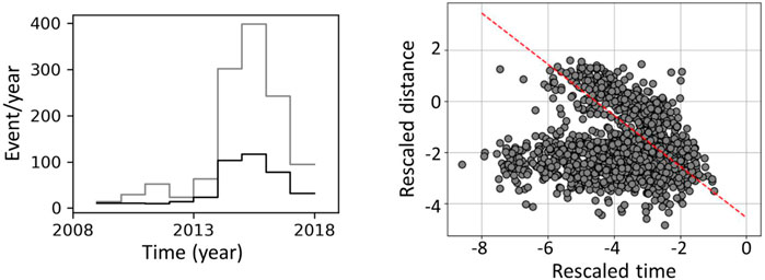
FIGURE 6. Declustering effect providing a separation between mainshocks and aftershocks induced by injection activities Left: all events of the catalogue (grey line) and independent mainshocks (black line). Right: Bimodal distribution of time and space components (
One of the assumptions in Dieterich’s seismicity rate theory (Dieterich, 1994) that is subject of debate, is the lack of interactions between seismic sources. More specifically, Dieterich’s seismicity rate theory assumes aftershocks are directly triggered by the stress changes induced by the mainshock. Effect of stress interactions between aftershocks is not accounted for. To circumvent this potential shortcoming of Dieterich’s theory, we apply the declustering algorithm of Zaliapin and co-workers (Zaliapin et al., 2008; Zaliapin and Ben-Zion 2013; Zaliapin and Ben-Zion, 2016). This algorithm resolves complete triggering chains based on the relative space-time-magnitude distances, originally introduced by Baiesi and Paczuski (2004). Only the main ingredients of the approach are given below, but the reader is referred to the papers of Zaliapin and co-workers for more details.
The declustering algorithm of Zaliapin et al. (2008) is based on space-time-magnitude distances between earthquakes
The nearest-neighbor distance for a given event
Zaliapin et al. (2008) proposed to consider the scalar distance
And now:
For our analysis, we fix
Zaliapin et al. (2008) and Zaliapin and Ben-Zion (2016) have shown that observed seismicity generally presents a bimodal joint distribution of (
2.5 Data assimilation
The objective of the data assimilation procedure is to determine the set(s) of model parameters [
The log-likelihood is defined as the logarithm of the probability that one specific model (with one specific set of model parameters) has generated the observed earthquake catalog. For each set of model parameters the posterior log-likelihood is calculated in order to rank the models (Ogata, 1998; Zhuang et al., 2012). The model with the highest log-likelihood is most likely to have generated the observed seismicity catalogue. For our non-homogeneous stationary Poisson process, and for a given time interval [t0, t1] and spatial area [x0,x1] × [y0,y1], the log-likelihood with respect to N observed earthquakes which have occurred at times ti and locations (xi,yi) is defined by the following function:
Following a Bayesian approach, and because we do not have a prior preference for the shape of the distribution of each model parameter, we attribute a bounded uniform probability distribution for each model parameter. The Markov Chain Monte Carlo (MCMC) algorithm is used to condition these uniform distributions with the observed seismicity.
The start of the time period where the data assimilation procedure is deployed is 1st January 2009, start of the observed seismicity, ending on 31 December 2017. Note that we apply our analysis to seismicity rate only. Incorporation of seismic magnitude requires further steps in the approach. Ideally, a joint log-likelihood is applied to assimilate both seismicity rate and seismic magnitude. However, in order to properly model the magnitude of induced events, a much more complex modelling strategy is required combining the nucleation rate from Dieterich’s (1994) theory with, for example, the state of stress and energy available around each nucleation point (e.g., Noda et al., 2009; Schmitt et al., 2015; Dempsey and Suckale, 2016). As performed in previous studies at Oklahoma (e.g., Zhai et al., 2019), the nucleation rate could be combined with an arbitrary frequency-magnitude distribution that is uniform and constant in space and time. However, applying such a procedure would bring additional uncertainties and, for the current purpose of the study, little added value. Therefore, we focus the analysis on nucleation rate of seismic events alone.
2.6 Constrained optimization
After applying the data assimilation procedure, the best set of model parameters can be selected with which our predictive model is more likely to explain the observed induced seismicity rate. Using this calibrated predictive model and set of model parameters, the optimum injection strategy is determined. The aim is to prevent the peak of seismicity kicking off in 2014, while at least the same volume of injected brine is injected as has been historically reported for the area. The objective is to maximize the total cumulative field-wide injected brine volume. We include a threshold value for the seismicity rate as a constraint that cannot be exceeded. The objective (maximizing injected volume) and the constraint (minimizing seismicity rate) are expected to be conflicting. The identification of an injection strategy that meets both our objective and constraint is a complex task. The complexity is increased by the non-regular distribution of wells, and the time-dependency of the geomechanical-seismological response (linking pore pressure diffusion and earthquake nucleation) to changes in injection rate. We therefore adopt a numerical optimization approach that aims to solve the following formalized problem:
The control vector
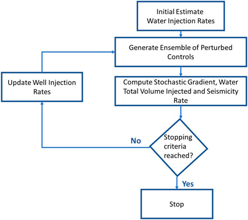
We use the Stochastic Simplex Approximate Gradient (StoSAG) estimation method where the gradients are used in an advanced method for constrained optimization (Chen et al., 2009; Fonseca et al., 2014, 2017). An ensemble of randomly chosen control vectors (well injection rates) is generated and the stochastic gradient, total volume of brine injected and yearly event rate are computed. Based on the stochastic gradient direction, the controls are updated, and a new ensemble of perturbed controls is regenerated. This iterative process continues until there are no more significant changes in the total amount of brine injected or controls, or when a maximum number of iterations is reached (Figure 7). As an initial estimate (i.e., first guess) for the controls we prescribe constant and equal rates for all wells, so that the cumulative injected volume is slightly lower than the historical total injected volume.
3 Results
3.1 Posterior model parameters of the unsteady Oklahoma fault system
The joint and marginal posterior probability distributions of the model parameters obtained after assimilation of the declustered catalogue over the period from 1st January 2009 to 31 December 2017 are well constrained (Figure 8). The median of the marginal posterior distributions of each model parameter define the best posterior estimates (
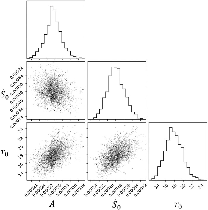
FIGURE 8. Posterior probability distributions of the seismicity rate model parameters obtained after the data assimilation procedure with the MCMC search. Histogram-type plot: marginal probability distribution of each individual parameter
The assimilation of observed events starts in 2009 when a significant earthquake activity started to be recorded. Consequently, the Dieterich (1994) seismicity rate Eq. 4 is solved assuming initial condition at steady state, that is
with the unsteady initial condition
3.2 Temporal pattern
A posterior ensemble of yearly event rate predictions can be visualized by randomly picking members from the posterior density distributions obtained with the MCMC search. This ensemble can be compared with the data. However, it should be noted that the modelling strategy does not yet include the intrinsic Poisson variability of earthquake occurrence. The observed declustered catalogue is considered here as one unique realization of a stochastic, non-stationary Poisson process. Each posterior member of the modelling approach is one particular model of the time-dependent seismicity rate underlying the Poisson process. For an appropriate assessment of the predictive performance of our models, the stochastic Poisson variabilities need to be accounted for. For each posterior member, which can be considered as the mean of an underlying Poisson distribution, multiple synthetic catalogues are generated where the likelihoods of the event location and timing are proportional to the event density (Zhuang and Touati, 2015). Figure 9 shows that the posterior predictions capture very well the temporal variation in observed seismicity. More specifically, our modelling strategy can predict:
(1) the relative seismicity quiescence from 2009 to 2013,
(2) the abrupt ramp-up of the seismicity rate starting in 2014,
(3) the fast decrease of the seismicity rate starting in 2016 with the new measures imposed by the regulators.
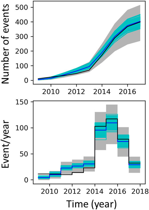
FIGURE 9. Comparison of the predicted seismicity histories with the data (black line). The model corresponds to 300 realizations (cyan) randomly drawn from the posterior density distribution obtained with the MCMC search during calibration. The mean of the models is indicated by the blue line. For each posterior member, 30 synthetic catalogues are generated in order to account for stochastic Poisson variabilities. The grey region indicates 95% of the distribution of the 9,000 synthetic catalogues when stochastic Poisson variabilities are accounted for. Top: cumulated number of events. Bottom: yearly event rate.
3.3 Spatial pattern
Predictions of spatial distribution of seismicity rate based on our modelling strategy can also be evaluated. Figure 10 show a comparison of the spatio-temporal distribution between observations and model predictions (i.e., event densities). The overall spatio-temporal evolution of the observed seismicity is well reproduced by our modelling strategy. More specifically, the observed and modelled seismicity both start to increase at the center of the area of interest (i.e., Central area) and then progressively migrate outwards to finally be concentrated in the North area.
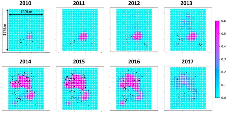
FIGURE 10. Mean posterior fields of event density (/cell) at 4 km depth along the basement faults. The black dots indicate the observed events.
3.4 Towards an optimum injection strategy
Now that parameters have been adjusted and that our model best explains the historical observations, this calibrated model can be used for the optimization exercises. Multiple optimization experiments have been performed but in the present manuscript we focus on the description of one key experiment. For this specific key experiment, we seek to find the optimum injection strategy for each well for the last 4 years [2013–2017] leading to a total volume of injected brine that is at minimum equal to the total historic injected volume while keeping the yearly event rate below a certain threshold. This threshold is set to 70 event/year in order to avoid the peak of seismicity rate starting in 2014. More specifically, the injection rate can be updated each year of the last 4 years independently for each well, which corresponds to 880 controls. For each iteration, the number of perturbations is set to 100 to appropriately compute the stochastic gradients. The optimizer successfully converged towards an optimum solution which satisfies both constraints: 1) the total volume injected is quasi-identical to the historical total volume injected, and 2) the yearly event rate is equal to the threshold of 70 event/year (Figure 11).
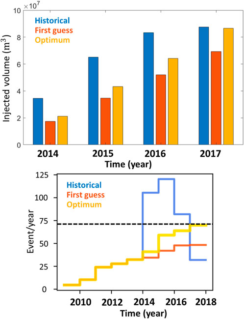
FIGURE 11. Comparison of the cumulative field-wide injected volumes (up) and seismicity rates (down) for the 4 years of the optimization period. The horizontal dashed line (bottom graph) indicates the imposed threshold of 70 event/year. Note that the historical seismicity rate (blue curve in bottom graph) is similar to the mean posterior (blue curve) in Figure 9.
Instead of preferentially using specific wells for most of the injected volume as historically, the optimum scenario suggests a more spatially uniform distribution of the injected volumes (see Figure 12).
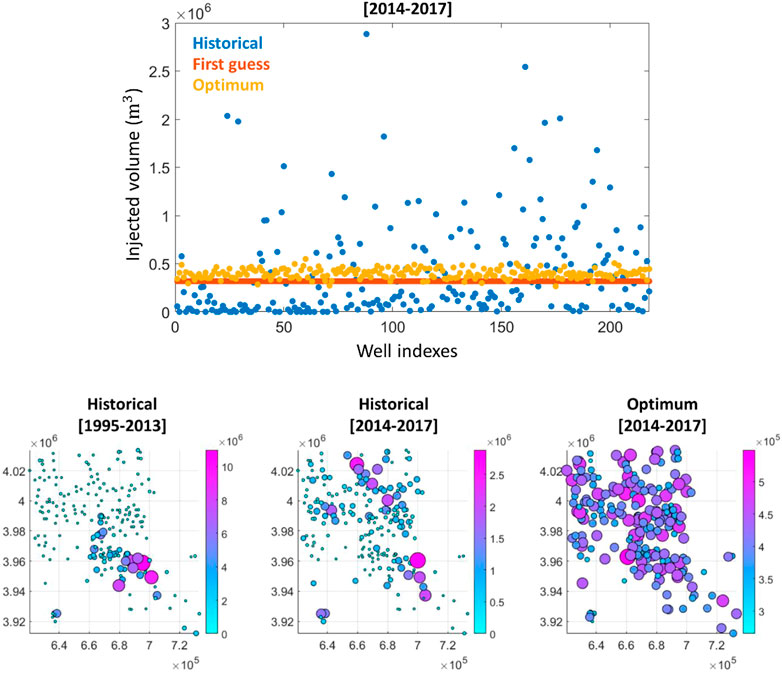
FIGURE 12. Comparison of the total injected volumes (m3) per wells. Note the range difference of each color scale in the bottom maps.
It is more interesting to identify any differences in the spatio-temporal pattern between the first guess scenario and optimum scenario. Indeed, the first guess scenario consists to the exact spatially uniform scenario where we prescribe constant and equal rates for all wells (see Figure 12). Therefore, any deviations from this first guess scenario should illuminate a non-uniform spatial pattern for the optimum scenario with preferential use of specific wells. It is difficult to draw conclusions solely based on the visual comparison of the event densities for the first guess and optimum strategies (see Figure 13). The spatial pattern seems identical for both strategies, except the overall higher event densities for the optimum scenario. However, and interestingly, plotting now the differences between the optimum and first guess event densities (see Figure 14), it appears clear that the optimizer preferentially used the wells of the North area. This optimum strategy can be explained by the fact that before the optimization period (that is before 2014) most of the wastewater have been injected in the Central area (see Figure 12) resulting in a very localized high event density in this area (see Figure 15). Therefore, the use of wells at the Central area has been penalized by the optimizer since additional stress changes in this area would have led to a yearly event rate which would have probably exceeded the threshold of 70 event/year.
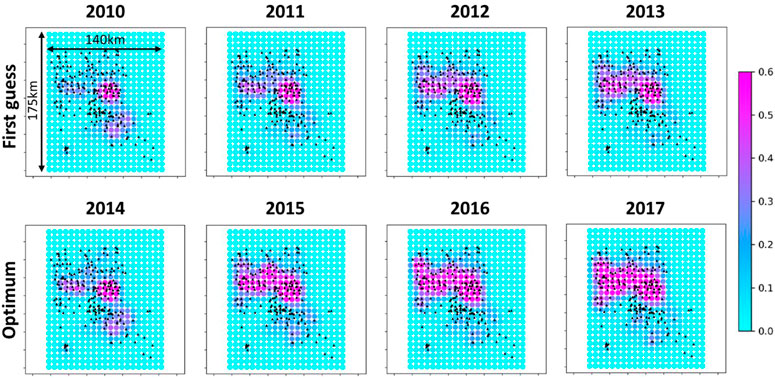
FIGURE 13. First guess and optimum event densities (/cell) at 4 km depth along the basement faults. The black triangles indicate the locations of the injector wells.

FIGURE 14. Difference between the event densities of the optimum and first guess scenarios. The grid cells underlined in black correspond to the ones with a high cumulative event density before the optimization period (see Figure 15).
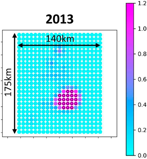
FIGURE 15. Cumulative event density (/cell) right before the start of the optimization period (end of 2013). Grid cells of the Central area with a number of events higher than 1.0 are underlined in black.
Figure 16 illustrates this last conclusion. Indeed, Figure 16 depicts, for the optimum scenario and one hypothetical scenario, typical stressing rate histories and relative seismicity rate histories for the Central area and North area. The hypothetical scenario illustrates the case where the injections and Coulomb stress rates would have been maintained in the Central area during the optimization period. In this hypothetical scenario the relative seismicity rate (already in a steady-state regime because of the high-injected volumes before 2014) would have been much higher than the optimum scenario, this last consisting in promoting injection in the North area.
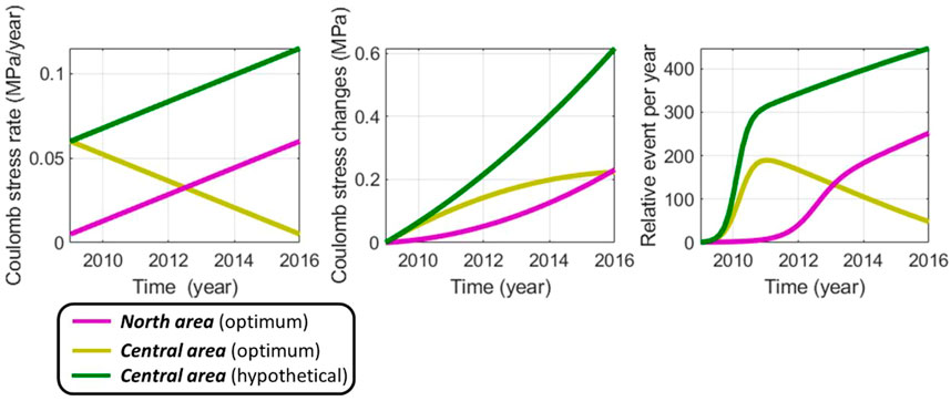
FIGURE 16. Synthetic examples of the Coulomb stress and relative event rate evolutions for the North area and Central area (see Figure 5). The Central area (optimum) curve and North area (optimum) curve illustrate the found optimum scenario. The Central area (hypothetical) corresponds to the hypothetical case where the injection would have been maintained in the Central area during the optimization period. By promoting the injection in the North area and releasing stresses in the Central area, the found optimum strategy prevents the high seismicity rates in the Central area.
Historically, even if the injected volumes have been progressively increased in the North area, a cluster of wells with high injected volumes has been continuously operating in the Central area (see Figure 12). These persistent high injected volumes in the Central area might explain the historical surge of seismicity at Oklahoma.
4 Concluding discussion
We present a three-step constrained optimization workflow that outlines injection scenarios for maximizing injected volume under a constraint imposed by seismicity rates. It represents a physics-based predictive workflow that ensures that simulated seismicity is consistent with observed seismicity. For high-volume wastewater injection around Oklahoma, the workflow can test multiple injection scenarios to find an optimum scenario which maximizes the total volume injected while avoiding the sharp increase of seismicity as observed in 2014. This increase led to the regulatory measures and ultimately to the shut-down of the injection.
In the first step of the workflow, a forward modelling strategy is designed that honors as much as possible all available knowledge from Oklahoma. It includes information on 1) geology and flow which are used to set up flow simulations, and 2) in situ stress conditions, fault orientations, observed seismicity and prime physical processes controlling it, which are used to deploy the geomechanical and seismological analysis. Flow simulations are performed by using the open source OPM-FLOW simulator which uses historical monthly injection rates of each well at Oklahoma as input. With the approach, robust spatio-temporal pressure distributions have been computed, including complex flow interaction between the 220 wells at Oklahoma. With the simulations, the pore pressure at the nucleation depth of seismic events in the basement was accurately captured. Based on the depth distribution of the observed events, an average depth of 4 km was selected for our analysis but note here that selecting an average nucleation depth slightly deeper, e.g., 5 km, would not have affected the conclusions of our analysis. The changes in pore pressure are the main drivers of the two physical processes controlling the nucleation of induced earthquakes in Oklahoma: the direct decrease in the effective normal stress at fault due to the pore pressure increase (Langenbruch and Zoback, 2016; Norbeck and Horne, 2016; Dempsey and Riffault, 2019), and the poro-elastic loading caused by the changes in the rock volume when its pore pressure is increased (Goebel et al., 2017a; Goebel et al., 2017b; Zhai et al., 2019). The stress contribution from the poro-elastic loading has been derived from the mechanical simulator MACRIS (Candela et al., 2019; van Wees et al., 2019). MACRIS is based on a newly developed mesh-free approach, which can 1) directly use 3D pressure fields from OPM-FLOW as input for geomechanical modelling, and 2) provide high stress resolution at the interface of interest (the horizontal-plane at 4 km depth in the Oklahoma case). Coulomb stress changes have been combined with Dieterich’s theory (Dieterich, 1994) to model the spatio-temporal evolution of the seismicity rate.
In the second step, the seismicity data are assimilated in order to update the model parameters of the forward model from the first step. Data assimilation is used to assess the predictive power of the forward model by comparing simulated and historical seismicity rates. This assimilation step has often not been considered in previous studies of induced seismicity at Oklahoma injection sites. Generally, a sensitivity analysis for temporal predictions of induced seismicity is performed (e.g., Zhai et al., 2019). In the current workflow, the seismicity data has been assimilated in both space and time (see also Candela et al., 2019). It has been demonstrated that the distribution of seismicity in both space and time can be used to constrain the posterior distributions of model parameters. We showed that 1) the field-wide modelled yearly event rate and 2) the modelled spatio-temporal event densities are both successfully capturing the spatio-temporal distributions of observed events. These results confirmed the predictive power of our modelling strategy that aims to honor the ensemble of available information for the Oklahoma injection sites. Although not performed in the present study, the results suggest that the approach is suitable to forecast the potential return of the Oklahoma induced seismicity to the background rate following the arrest of all injection activities (Langenbruch et al., 2018; Zhai et al., 2019).
In the third step, an optimization approach is outlined that aims to find an optimum spatio-temporal injection scheme in order to maximize the total volume injected while keeping the seismicity rate below a cap. The cap is chosen so that the stop of the injection activities in April 2017 may be prevented as seismicity remains below a threshold value.
The present study combines both cutting-edge physics-based predictive models with a cutting-edge optimization algorithm. Despite that the modelling framework is applied to the Oklahoma case study, the primary objective was to demonstrate that complex optimization problems with two conflicting objectives involving full physics-based models for flow, geomechanics and induced seismicity can be solved. The modelling framework is based on existing workflows that were originally deployed for the optimization of well planning for hydrocarbon recovery (Chen et al., 2009; Fonseca et al., 2014, 2017), and adjusted for our specific constrained optimization problem. As such this modelling framework can thus be seen as generic and can be applied to other instances of anthropogenic subsurface activities as for example but not limited to that carbon storage and sequestration.
We showed that it likely would have been possible to avoid the dramatic rise of the rate of seismicity starting in 2014 while still injecting a total volume of fluid identical to the historical injected volume. The optimum strategy involved more uniform spatio-temporal distributions of the injection rates. More specifically the optimizer suggested to prevent the injection of additional large volumes in the Central area because already at steady-state seismicity rate due to large fluid-volumes injected before 2014.
More constraints should be added to the present approach in order to include additional key factors which have influenced the spatio-temporal historical distribution of the injection rates. As an example, the use of wells for injection should be constrained by additional parameters such as the supply of hydraulic fracturing and formation fluids from nearby hydrocarbon industry activities and notably shale gas sites as the fluid brine injected in the Arbuckle aquifer is a waste-product of production of shale gas. Accordingly, a spatio-temporal correlation between injection volumes and hydrocarbon industry operations in the area is likely. In the current optimization example, it is assumed that all wells were available at any moment in time. One way to honor the correlation between hydrocarbon industry operations and injection is to add a cost constraint in the optimization, i.e., injections via wells that were not used in historical injection should be penalized with a higher cost. This additional implementation can be achieved with the present optimization algorithm.
Data availability statement
The raw data supporting the conclusion of this article will be made available by the authors, without undue reservation.
Author contributions
TC: Conception and design of the work; Acquisition, analysis, and interpretation of data for the work; Drafting the work. CG: Conception and design of the work; Acquisition, analysis, and interpretation of data for the work; Drafting the work. OL: Conception and design of the work; Interpretation of data for the work; Drafting the work. JT: Drafting the work.
Acknowledgments
This work is part of the SECURE project. The data generated by the integrated approach are available on request from the corresponding author. We thank the Oklahoma Corporate Commission (OCC) and Oklahoma Geological Survey (OGS) for making publicly available respectively the disposal well data and the earthquake catalog (https://www.ou.edu/ogs).
Conflict of interest
The authors declare that the research was conducted in the absence of any commercial or financial relationships that could be construed as a potential conflict of interest.
Publisher’s note
All claims expressed in this article are solely those of the authors and do not necessarily represent those of their affiliated organizations, or those of the publisher, the editors and the reviewers. Any product that may be evaluated in this article, or claim that may be made by its manufacturer, is not guaranteed or endorsed by the publisher.
References
Ader, T., Lapusta, N., Avouac, J.-P., and Ampuero, J. P. (2014). Response of rate-and-state seismogenic faults to harmonic shear-stress perturbations. Geophys. J. Int. 198 (1), 385–413. doi:10.1093/gji/ggu144
Alt, R. C., and Zoback, M. D. (2016). In situ stress and active faulting in Oklahoma. Bull. Seismol. Soc. Am. 107 (1), 216–228. doi:10.1785/0120160156
Baiesi, M., and Paczuski, M. (2004). Scale-free networks of earthquakes and aftershocks. Phys. Rev. E 69, 066106. doi:10.1103/physreve.69.066106
Barnes, J., and Hut, P. (1986). A hierarchical O(N log N) force-calculation algorithm. Nature 324, 446–449. doi:10.1038/324446a0
Candela, T., Osinga, S., Ampuero, J. P., Wassing, B., Pluymaekers, M., Fokker, P. A., et al. (2019). Depletion-induced seismicity at the Groningen gas field: Coulomb rate-and-state models including differential compaction effect. J. Geophys. Res. Solid Earth 124, 7081–7104. doi:10.1029/2018jb016670
Chen, Y., Oliver, D. S., and Zhang, D. (2009). Efficient ensemble-based closed-loop production optimization. SPE J. 14 (4), 634–645. doi:10.2118/112873-pa
Dempsey, D., and Suckale, J. (2016). Collective properties of injection-induced earthquake sequences: 1. Model description and directivity bias. J. Geophys. Res. 121 (5), 3609–3637. doi:10.1002/2015JB012550
Dempsey, D., and Riffault, J. (2019). Response of induced seismicity to injection rate reduction: Models of delay, decay, quiescence, recovery, and Oklahoma. Water Resour. Res. 55, 656–681. doi:10.1029/2018WR023587
Dieterich, J. H., and Kilgore, B. (1996). Implications of fault constitutive properties for earthquake prediction. Proc. Natl. Acad. Sci. U. S. A. 93 (9), 3787–3794. doi:10.1073/pnas.93.9.3787
Dieterich, J. H. (1994). A constitutive law for rate of earthquake production and its application to earthquake clustering. J. Geophys. Res. 99, 2601–2618. doi:10.1029/93jb02581
Ellsworth, W. L. (2013). Injection-induced earthquakes. Science 341, 1225942. doi:10.1126/science.1225942
Faith, J. R., Blome, C. D., Pantea, M. P., Puckette, J. O., Halihan, T., Osborn, N., et al. (2010). Three-dimensional geologic model of the Arbuckle-Simpson Aquifer, south-central Oklahoma. US Geological Survey. USGS report. Available at: https://pubs.usgs.gov/of/2010/1123/downloads/Report/OF10-1123.pdf.
Firkins, M., Kolawole, F., Marfurt, K. J., and Carpenter, B. M. (2020). Attribute assisted characterization of basement faulting and the associated sedimentary sequence deformation in north-central Oklahoma. Interpretation 8, SP175–SP189. doi:10.1190/INT-2020-0053.1
Fonseca, R. M., Stordal, A. S., Leeuwenburgh, O., Van den Hof, P. M. J., and Jansen, J. D. (2014). “Robust ensemble-based multi-objective optimization,” in ECMOR XIV-14th European conference on the mathematics of oil recovery. Sicily, Italy, September 8–11, 2014.
Fonseca, R. R. M., Chen, B., Jansen, J. D., and Reynolds, A. (2017). A stochastic simplex approximate gradient (StoSAG) for optimization under uncertainty. Int. J. Numer. Meth. Engng. 109 (13), 1756–1776. doi:10.1002/nme.5342
Geertsma, J. (1973). A basic theory of subsidence due to reservoir compaction: the homogeneous case. Verh. Kon. Ned. Geol. Mijnbouwkd. Genoot. 28, 43–62.
Goebel, T. H. W., Weingarten, M., Chen, X., Haffner, J., and Brodsky, E. E. (2017a). The 2016 Mw5.1 Fairview, Oklahoma earthquakes: Evidence for long-range poro-elastic triggering at >40 km from fluid disposal wells. Earth Planet. Sci. Lett. 472, 50–61. doi:10.1016/j.epsl.2017.05.011
Goebel, T. H. W., Walter, J., Murray, K., and Brodsky, E. E. (2017b). Comment on: How will induced seismicity in Oklahoma respond to decreased saltwater injection rate. Sci. Adv. 3, e1700441. doi:10.1126/sciadv.1700441
Hicks, A. (2011). Clustering in multidimensional spaces with applications to statistical analysis of earthquake clustering. MSc Thesis. Reno: Department of Mathematics and Statistics, University of Nevada.
Hincks, T., Aspinall, W., Cooke, R., and Gernon, T. (2018). Oklahoma’s induced seismicity strongly linked to wastewater injection depth. Science 359, 1251–1255. doi:10.1126/science.aap7911
Holland, A. A. (2013). Optimal Fault orientations within Oklahoma. Seismol. Res. Lett. 84 (5), 876–890. doi:10.1785/0220120153
Johann, L., Shapiro, S. A., and Dinske, C. (2018). The surge of earthquakes in Central Oklahoma has features of reservoir-induced seismicity. Sci. Rep. 8, 11505. doi:10.1038/s41598-018-29883-9
Johnson, K. S. (2008). “Geologic history of Oklahoma,” in Earth sciences and mineral resources of Oklahoma (Oklahoma Geological Survey Educational Publication), 9, 3–5. 346.
Keranen, K. M., Savage, H. M., Abers, G. A., and Cochran, E. S. (2013). Potentially induced earthquakes in Oklahoma, USA: Links between wastewater injection and the 2011 Mw 5.7 earthquake sequence. Geology 41 (6), 699–702. doi:10.1130/g34045.1
Keranen, K. M., Weingarten, M., Abers, G. A., Bekins, B. A., and Ge, S. (2014). Sharp increase in central Oklahoma seismicity since 2008 induced by massive wastewater injection. Science 345, 448–451. doi:10.1126/science.1255802
Kolawole, F., Johnson, C., Chang, J. C., Marfurt, K. J., Lockner, D. A., Reches, Z., et al. (2019). The susceptibility of Oklahoma’s basement to seismic reactivation. Nat. Geosci. 12, 839–844. doi:10.1038/s41561-019-0440-5
Langenbruch, C., and Zoback, M. D. (2016). How will induced seismicity in Oklahoma respond to decreased saltwater injection rates? Sci. Adv. 2, e1601542. doi:10.1126/sciadv.1601542
Langenbruch, C., Weingarten, M., and Zoback, M. D. (2018). Physics-based forecasting of manmade earthquake hazards in Oklahoma and Kansas. Nat. Commun. 9, 3946. doi:10.1038/s41467-018-06167-4
Marone, C. (1998). Laboratory-derived friction laws and their application to seismic faulting. Annu. Rev. Earth Planet. Sci. 26, 643–696. doi:10.1146/annurev.earth.26.1.643
McGarr, A., and Barbour, A. J. (2017). Wastewater disposal and the earthquake sequences during 2016 near Fairview, Pawnee, and Cushing, Oklahoma. Geophys. Res. Lett. 44, 9330–9336. doi:10.1002/2017gl075258
Mindlin, R. D. (1936). Force at a point in the interior of a semi infinite Solid. Physics 7, 195–202. doi:10.1063/1.1745385
Noda, H., Dunham, E. M., and Rice, J. R. (2009). Earthquake ruptures with thermal weakening and the operation of major faults at low overall stress levels. J. Geophys. Res. 114, B07302. doi:10.1029/2008JB006143
Norbeck, J. H., and Horne, R. N. (2016). Evidence for a transient hydromechanical and frictional faulting response during the 2011Mw 5.6 Prague, Oklahoma earthquake sequence. J. Geophys. Res. Solid Earth 121, 8688–8705. doi:10.1002/2016JB013148
Ogata, Y. (1998). Space-time point-process models for earthquake occurrences. Ann. Inst. Stat. Math. 50 (2), 379–402. doi:10.1023/a:1003403601725
Okada, Y. (1992). Internal deformation due to shear and tensile faults in a half-space. Bull. Seismol. Soc. Am. 82 (2), 1018–1040. doi:10.1785/bssa0820021018
Pei, S., Peng, Z., and Chen, X. (2018). Locations of injection-induced earthquakes in Oklahoma controlled by crustal structures. J. Geophys. Res. Solid Earth 123, 2332–2344. doi:10.1002/2017jb014983
Qin, Y., Chen, X., Walter, J. I., Haffener, J., Trugman, D. T., Carpenter, B. M., et al. (2019). Deciphering the stress state of seismogenic faults in Oklahoma and southern Kansas based on an improved stress map. J. Geophys. Res. Solid Earth 124, 12920–12934. doi:10.1029/2019JB018377
Rasmussen, A. F., Sandve, T. H., Bao, K., Lauser, A., Hove, J., Skaflestad, B., et al. (2021). The open porous media flow reservoir simulator. Comput. Math. Appl. 81, 159–185. doi:10.1016/j.camwa.2020.05.014
Schmitt, S. V., Segall, P., and Dunham, E. M. (2015). Nucleation and dynamic rupture on weakly stressed faults sustained bythermal pressurization. J. Geophys. Res. Solid Earth 120 (11), 7606–7640. doi:10.1002/2015JB012322
Segall, P., and Lu, S. (2015). Injection-induced seismicity: Poro-elastic and earthquake nucleation effects. J. Geophys. Res. Solid Earth 120, 5082–5103. doi:10.1002/2015JB012060
van Wees, J. D., Osinga, S., Van Thienen-Visser, K., and Fokker, P. A. (2018). Reservoir creep and induced seismicity: inferences from geomechanical modeling of gas depletion in the groningen field. Geophys. J. Int. 212, 1487–1497. doi:10.1093/gji/ggx452
van Wees, J. D., Pluymaekers, M., Osinga, S., Fokker, P. A., Van Thienen-Visser, K., Orlic, B., et al. (2019). 3-D mechanical analysis of complex reservoirs: A novel mesh-free approach. Geophys. J. Int. 219, 1118–1130. doi:10.1093/gji/ggz352
Walsh, F. R., and Zoback, M. D. (2015). Oklahoma’s recent earthquakes and saltwater disposal. Sci. Adv. 1, e1500195. doi:10.1126/sciadv.1500195
Weingarten, M., Ge, S., Godt, J. W., Bekins, B. A., and Rubinstein, J. L. (2015). High-rate injection is associated with the increase in U.S. mid-continent seismicity. Science 348, 1336–1340. doi:10.1126/science.aab1345
Zaliapin, I., and Ben-Zion, Y. (2013). Earthquake clusters in southern California, I: Identification and stability. J. Geophys. Res. Solid Earth 118, 2847–2864. doi:10.1002/jgrb.50179
Zaliapin, I., and Ben-Zion, Y. (2016). Discriminating characteristics of tectonic and human-induced seismicity. Bull. Seismol. Soc. Am. 106 (3), 846–859. doi:10.1785/0120150211
Zaliapin, I., Gabrielov, A., Keilis-Borok, V., and Wong, H. (2008). Clustering analysis of seismicity and aftershock identification. Phys. Rev. Lett. 101, 018501. doi:10.1103/PhysRevLett.101.018501
Zhai, G., Shirzaei, M., Manga, M., and Chen, X. (2019). Pore-pressure diffusion, enhanced by poro-elastic stresses, controls induced seismicity in Oklahoma. Proc. Natl. Acad. Sci. U. S. A. 116 (33), 16228–16233. doi:10.1073/pnas.1819225116
Zhuang, J., and Touati, S. (2015). “Stochastic simulation of earthquake catalogs,” in Community online resource for statistical seismicity analysis. Available at: http://www.corssa.org. doi:10.5078/corssa-43806322
Keywords: induced seimicity, pressure diffusion, poroelasticity, rate- and state-dependent friction, data assimilation, optimization
Citation: Candela T, Goncalves Machado C, Leeuwenburgh O and Ter Heege J (2022) A physics-informed optimization workflow to manage injection while constraining induced seismicity: The Oklahoma case. Front. Earth Sci. 10:1053951. doi: 10.3389/feart.2022.1053951
Received: 26 September 2022; Accepted: 10 November 2022;
Published: 28 November 2022.
Edited by:
Nicola Tisato, The University of Texas at Austin, United StatesReviewed by:
Nadine Igonin, The University of Texas at Austin, United StatesBrett Carpenter, University of Oklahoma, United States
Copyright © 2022 Candela, Goncalves Machado, Leeuwenburgh and Ter Heege. This is an open-access article distributed under the terms of the Creative Commons Attribution License (CC BY). The use, distribution or reproduction in other forums is permitted, provided the original author(s) and the copyright owner(s) are credited and that the original publication in this journal is cited, in accordance with accepted academic practice. No use, distribution or reproduction is permitted which does not comply with these terms.
*Correspondence: Thibault Candela, dGhpYmF1bHQuY2FuZGVsYUB0bm8ubmw=
 Thibault Candela
 Cintia Goncalves Machado
 Olwijn Leeuwenburgh
