
94% of researchers rate our articles as excellent or good
Learn more about the work of our research integrity team to safeguard the quality of each article we publish.
Find out more
ORIGINAL RESEARCH article
Front. Earth Sci., 12 January 2023
Sec. Paleontology
Volume 10 - 2022 | https://doi.org/10.3389/feart.2022.1046327
 Xiong Duan1,2*
Conodonts are jawless vertebrates deposited in marine strata from the Cambrian to the Triassic that play an important role in geoscience research. The accurate identification of conodonts requires experienced professional researchers. The process is time-consuming and laborious and can be subjective and affected by the professional level and opinions of the appraisers. The problem is exacerbated by the limited number of experts who are qualified to identify conodonts. Therefore, a rapid and simple artificial intelligence method is needed to assist with the identification of conodont species. Although the use of deep convolutional neural networks (CNN) for fossil identification has been widely studied, the data used are usually from different families, genera or even higher-level taxonomic units. However, in practical geoscience research, geologists are often more interested in classifying species belonging to the same genus. In this study, we use five fine-grained CNN models on a dataset consisting of nine species of the conodont genus Hindeodus. Based on the cross-validation results, we show that using the Bilinear-ResNet18 model and transfer learning generates the optimal classifier. Area Under Curve (AUC) value of 0.9 on the test dataset was obtained by the optimal classifier, indicating that the performance of our classifier is satisfactory. In addition, although our study is based on a very limited taxa of conodonts, our research principles and processes can be used as a reference for the automatic identification of other fossils.
Fossils are defined as paleontological remains and active remains preserved in rocks. They provide an important basis for the study of the origin of life, biological evolution, stratigraphic age, the paleogeographic environment, plate tectonics, oil and gas exploration and other scientific topics (Du and Tong, 2009). Fossil identification is particularly important for accurately obtaining key taxonomic knowledge for biostratigraphic analysis and to better serve earth science research. The general process of fossil identification is as follows: experts familiar with a particular genus examine the external morphology and internal structure of a fossil, consult the relevant paleontological literature, compare it with previous fossil specimens, plates and descriptions, and rely on their own experience to identify the species. The traditional process of fossil identification usually relies too much on the prior knowledge of experts, and is time consuming, labor intensive, and subjective. For earth science researchers without a background in paleontology, the challenge of accurately identifying fossils may be one of the factors that slows their progress. Paleontologists can only identify species with which they are familiar and the expertise of paleontologists is usually limited to a specific taxon. The reality is that the proportion of researchers in the field of geology with a background in paleontology is small, but there is a huge demand for fossil identification for both scientific research and industrial production. This problem is becoming increasingly prominent.
With the digitization of geological specimen images, the application of big data mining and machine learning in the field of geosciences has been improved and broadened (Zhou et al., 2018), and the potential application of computer vision in paleontology has also attracted much attention. Numerous studies have shown that the performance of machines in image recognition is comparable to that of humans and machines become more efficient and accurate as computing power and data increase (LeCun et al., 2015). Therefore, in this work, we use theoretical knowledge of machine learning and deep learning to find an efficient and accurate intelligent fossil identification model, which can greatly simplify the traditional fossil identification process and allow people without paleontological knowledge to identify fossils.
The most serious biological extinction since the Cambrian explosion at the end of the Permian period has been studied in many aspects, and clarifying the boundary between the Permian and Triassic is the basis of all research work. In this paper, we use a variety of fine-grained CNNs to automatically identify the genus Hindeodus, which can help to clarify the boundary between the Permian and Triassic to some extent. In addition, although our study is based on conodonts, our research principles and processes can be used as a reference for the intelligent identification of other fossils.
Intelligent identification of paleontological fossils mainly relies on machine learning models and deep learning models in the field of computer vision. In recent decades, scholars in different research fields have tried to use various shallow machine learning models for intelligent image recognition (Sinha, 1998; de Vel and Aeberhard, 2000; Ryu and Oh, 2001; Dong et al., 2002; Ng and Gong, 2002; Kotropoulos and Pitas, 2003; Casasent and Wang, 2005; Long et al., 2006; Inglada, 2007; Shen and Liu, 2008; Suresh et al., 2009; Minhas et al., 2010; Mohammed et al., 2011). However, the algorithm in traditional machine learning image feature extraction is usually designed based on the specific application conditions and the guidance and suggestions of professionals. The modeling process is complex and the generalization ability and robustness of the model are often unsatisfactory (LeCun et al., 2015). In recent years, thanks to the significant increase in computing power, deep learning models, especially CNN models, have been developed rapidly and have exhibited good performance in multiclass image automatic recognition tasks. Deep learning has also been applied in some areas previously dominated by traditional machine learning. In 2012, a remarkable CNN called AlexNet was proposed in the field of deep learning and achieved top-1 and top-5 error rates of 37.5% and 17.0% on the ImageNet dataset, respectively (Krizhevsky et al., 2012). Since then, many classical CNNs have emerged, such as VGGNet (Simonyan and Zisserman, 2015), GoogLeNet (Szegedy et al., 2015), ResNet (He et al., 2016), and DenseNet (Huang et al., 2017). These CNNs generally show a trend of deeper and deeper network layers and more complex network architectures, all of which play an important role in image recognition tasks, while the application of these CNNs in fields such as medicine, agriculture, and transportation has greatly contributed to the development of deep learning. Not coincidentally, increasingly sophisticated CNNs are widely used in various fields of geology, such as paleontological fossil identification (Keçeli et al., 2018; de Lima et al., 2019; Hsiang et al., 2019; Mitra et al., 2019; Bourel et al., 2020; Liu et al., 2020; Marchant et al., 2020; Pires de Lima et al., 2020; Romero et al., 2020; An et al., 2022; Liu et al., 2022; Wang et al., 2022), geological prospecting (Li et al., 2020; Li et al., 2021), carbonate microfacies analysis (Liu and Song, 2020), and mineral rock identification (Xu and Zhou, 2018; Zhang et al., 2018; Baraboshkin et al., 2020; Guo et al., 2020; Alférez et al., 2021).
Based on previous research results, the classifiers trained on the paleontological fossil dataset with deep learning network models achieved high accuracy. Bourel et al. (2020) used multiple-CNNs to identify and classify eight modern pollen grains as well as fossil pollen grains from East Africa, achieving 100% accuracy on a dataset of all intact pollen grains and 97.2% and 96.7 accuracy on a dataset containing damaged pollen grains and a dataset with fossil pollen grains, respectively. Mitra et al. (2019) performed automatic identification of six extant planktonic foraminifera extensively studied by paleoceanographers, and manual screening was performed by experts and novices in their study; their study showed that the accuracy of automatic identification was slightly higher than that of expert identification and much higher than that of novice identification, but the precision and recall of manual identification were much lower than those of automatic identification due to limitations in a priori knowledge. Keçeli et al. (2018) used a pretrained VGG16 network model with fine-tuning to achieve an accuracy of 90.22% on the fossil radiolarian dataset. Hsiang et al. (2019) trained 27,737 images of modern planktonic foraminifera using three CNNs, VGG16, DenseNet121 and Inception V3, and the best performing classifier obtained correct species names for 87.4% of the images on the test set (a total of 6,903 images). Pires De Lima et al. (2020) used five pretrained network models, VGG19 and ResNet50, and fine-tuned them to train and test a total of 342 fusulinid fossil images of 8 classes in the late Paleozoic, showing that given sufficient data for training, the CNN model can correctly identify fusulinid fossils with high accuracy (>80%). Liu et al. (2020) used five network models, ResNet-18, ResNet-34, ResNet-50, ResNet-101, and ResNet-152, and employed transfer learning to train on a dataset of eight Ordovician conodonts with a total of 1761 image data and tested the models using 205 data points. The results showed that the accuracy of all models exceeded 80%, but illustrated that increasing the network depth did not necessarily improve the accuracy and that transfer learning was more favorable than training from scratch (Liu et al., 2020). An et al. (2022) performed hierarchical intelligent recognition of four Mesozoic ostracoid fossils, Dongyingia florinodosa, Dongyingia biglobicostat, Phacocypris guangraoensis, and Berocypris substriala (i.e., fossils were first target detection for initial classification and then applied CNN and SVM for more detailed classification on this basis) with a final recognition accuracy of 95%. Wang et al. (2022) designed a transpose CNN based on a fully convolutional network (Long et al., 2015) and U-NET (Ronneberger et al., 2015) for the automatic identification of brachiopod fossils, which were compared and analyzed. The network was applied to a small dataset of brachiopod fossils.
The above research results are exciting and indicate that the deep learning network model can be applied to the identification of paleontological fossils. The fossil data used previously for automatic identification all came from different genera or families or even higher-level taxonomic units. Due to the large differences in the characteristics (such as texture, shape, etc.) of different categories of samples and the small number of categories, machines can relatively easily and accurately identify the sample category with a high accuracy rate. Even ordinary geologists can identify these differences, such as distinguishing between bivalves and foraminifera. However, fossil identification in earth science research requires identification of more closely related species. Since researchers usually study a particular section of stratigraphy, the collected fossil samples are inevitably concentrated in several genera or represent multiple species within a genus, and the identification of fossils between species within a genus is often the focus and challenge of the identification task. Based on the above considerations, we recommend that all fossils whose data is used for CNN model training be of the same genus, and the dataset be as complete as possible to include all species belonging to the genus to maximize the usefulness of the model.
The above problem highlights another Frontier research hotspot in deep learning image recognition, namely, fine-grained image recognition (FGIR), also known as subcategory image recognition. In data settings with limited training data and highly similar data, the unsatisfactory results obtained using classical CNN models alone led to the rapid development of FGIR in computer vision in the last decade (Luo and Wu, 2017; Wei et al., 2022a). FGIR aims to distinguish numerous visually similar subordinate categories belonging to the same basic class, which is extremely challenging [especially the classification of visually sensory similar objects (Wei et al., 2022a)] but also has great application prospects, such as for automatic biodiversity monitoring (Van Horn et al., 2021), intelligent retail (Wei et al., 2022b), and intelligent transportation (Khan and Ullah, 2019).
Compared with generic image recognition, fine-grained image recognition objects mainly have two characteristics (Figure 1): the difference between classes is small, that is, all data belong to a subclass of the same class; and due to the influence of object pose, scale and photo angle, there are great intraclass differences. So, fine-grained image recognition must capture more subtle differences.
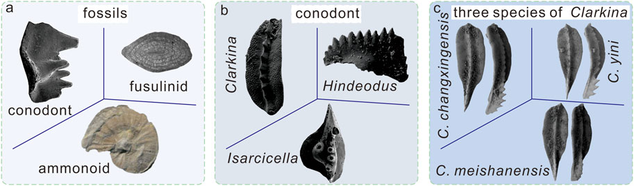
FIGURE 1. Schematic diagram of different grained images. (A) Coarse -grained images, all fossils belong to different classes, fusulinid provided by Arefifard and Payne (2020), ammonoid provided by Shi et al. (2017). (B) Middle -grained images, all conodonts belong to different genera. (C) Fine-grained images, all conodonts belong to same genus, these three species of conodont genus Clarkina are provided by Yuan and Shen (2011).
Based on the amount of supervised information used, FGIR can be divided into strongly supervised and weakly supervised FGIR. Strongly supervised FGIR algorithms are those that use additional manual annotation of feature information such as bounding boxes and part annotation in addition to the basic image category labels during model training. The detection of foreground objects can be accomplished with the help of the bounding box, thus eliminating the interference of background noise, while part annotation can be used to locate some useful local areas to achieve local feature extraction. Representative CNN models for strongly supervised information FGIR are deep convolutional activation feature (DeCAF) (Donahue et al., 2014), part-based R-CNN (Zhang et al., 2014), pose normalized CNN (Branson et al., 2014) and mask-CNN based on part segmentation model (Wei et al., 2018).
The usefulness of strongly supervised models is limited by the cost of labeling information acquisition, the need for professional assistance, and the considerable cost in terms of time and effort. The use of weakly supervised fine-grained models have become the main trend of fine-grained image research in recent years and they can achieve good classification performance compared to that of strongly supervised network models without the help of manual annotation information and by relying only on category labels. The principle behind weakly supervised fine-grained classification models is similar to that of strongly supervised classification models, and they also require global and local information to perform fine-grained level classification. The difference is that weakly supervised fine-grained models extract this information completely by computer, without human involvement during the process. Representative models for fine-grained classification with weakly supervised information are two-level attention in CNNs (Xiao et al., 2015), constellations of neural activations (Simon and Rodner, 2015), bilinear CNNs (Lin et al., 2015) and improved models (Gao et al., 2016; Lin and Maji, 2017).
In summary, in the process of fine-grained image classification, whether by supervised or unsupervised feature learning, the effective extraction of key local information is essential for the model’s ability to achieve good results. As a result of continuous research on unsupervised classification models, their accuracy rates are comparable to those of supervised models, and they have been more widely used in various fields because they eliminate the need for human involvement in model training.
The data used for this study were from samples of some species of the conodont genus Hindeodus, which were deposited during the Permian‒Triassic transition. Conodonts are jawless vertebrates found throughout marine strata from the Cambrian to Triassic, many of which are index fossils for stratigraphic division and correlation. In addition, the conodont color alteration index plays an important role in the evolution of sedimentary environments, interpretation of basin histories, regional metamorphic studies, and petroleum exploration (Epstein et al., 1977).
Conodont scanning electron microscopy (SEM) image data were obtained from published literature (an appendix file provided for original references) and our own SEM images obtained from rock samples. When collecting conodont image data, the quality of the images was strictly controlled, including the resolution of the images and the intactness of the fossils themselves, meaning that low-resolution and severely incomplete fossils were not included in the dataset. In addition, when the number of a species collected was small, the data were not included the dataset. Based on the above two conditions for selecting conodonts, a total of 613 images from only the following nine species were selected for inclusion in the dataset in this study (Figure 2): H. changxingensis, H. eurypyge, H. inflatus, H. julfensis, H. latidentatus, H. parvus, H. praeparvus, H. sosioensis, and H. typicalis.
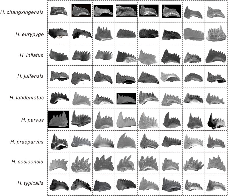
FIGURE 2. Example illustrations of each species of the conodont genus Hindeodus in the dataset.
For the same conodont sample, the sample provider usually shows SEM images from three perspectives: lateral view, upper view and lower view. In this study, only the lateral view image was selected because it best reflects the characteristics of the fossil. Before training, we did not do the raw data for offline enhancement, but used the methods of PyTorch framework (e.g., Random Resized Crop and Random Horizontal Flip) for data enhancement during training.
When performing image classification tasks, the general practice is to divide the dataset into a training set, validation dataset and test dataset. The training dataset is used to train the model and to determine the parameters (i.e., weight and bias) of the model; the validation dataset is used to adjust the hyperparameters (e.g., learning rate, epoch, batch size) during model training and determine when to stop training based on the convergence of the model; the test dataset contains data that have never been seen during the model training process and is not used in the training of the model, but is used for the final evaluation of the generalization ability of the model. The above division of datasets is usually feasible when the amount of data is sufficient. The conodont dataset collected in this study has two problems: the dataset is small and imbalanced. In the case of a small dataset, if the above division scheme is used, feature learning will not use as much data as possible and the validation results of the model may have a large degree of randomness; cross-validation can be a good solution to this problem. There are various forms of cross-validation. In K-fold cross-validation, the test set is retained, but in the model training process, instead of setting aside a fixed validation set, the training set is equally divided into K blocks. In each iteration, K-1 blocks are used as the training set, and the remaining block is used as the validation set, so that the CNN model is trained and validated K times. Then, the average accuracy calculated from the accuracy of the K iterations is used as the performance measure of the model. When the dataset is unbalanced in all classes, the use of stratified sampling as implemented in stratified K-fold cross-validation is recommended to ensure that relative class frequencies are approximately preserved in each training and validation set (Figure 3).
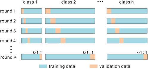
FIGURE 3. Schematic diagram of Stratified K-fold cross validation.
In this paper, we used a stratified K-fold cross-validation approach for model selection (including hyperparameter determination) and divided the conodont data into a training dataset (∼85% of the data) and a test dataset (∼15% of the data) without dividing the validation set separately (Table 1). The division of the dataset was implemented in the following steps: 1) create two folders on the local disk named the training dataset and test dataset; 2) create 9 subfolders in the training dataset and test dataset folders, each with a name corresponding to the names of the above 9 classes of conodonts; and 3) put 85% of the data of each class of conodonts into the corresponding subfolder in the training dataset and the other 15% into the corresponding subfolder in the test dataset.
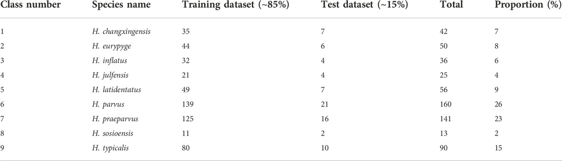
TABLE 1. Species of the conodont genus Hindeodus used for the classification and the number of images per species in the constructed dataset.
In feature learning with models of high complexity, if there is not enough data available for training the models, the trained models often suffer from overfitting (i.e., they perform well on the training set but do not generalize well on the test set and new data). The best way to avoid overfitting is to obtain more training data; however, in some highly specialized scenarios, it is often difficult to obtain enough data. The most common means of preventing model overfitting is to use model-based migration learning (i.e., parameter-based migration learning) in addition to adding data. It can save computational resources and improve computations, which usually also improves the accuracy rate. When training new data with a CNN model, it is possible to use a pretrained model (typically one that has been trained on a large dataset such as ImageNet) as a feature extractor and replacing the final output layer of the model (usually the last fully connected layer). Since the previous layers in a convolutional neural network extract generic features, to extract specific features from specialized data, the previous layers can be frozen while retraining the last layers of the network in a method known as fine-tuning.
To further prevent overfitting of the model during training, weight decay and dropout are used for model training. Weight decay is like L2 regularization, which reduces the weight in the neural network and is a common approach for dealing with overfitting. In the PyTorch framework, weight decay is represented as a parameter in the optimizer, and the value of weight decay was set to 0.00001 in the experiment. Dropout refers to an approach to the training of the model in which the neural network units are temporarily dropped from the network with a certain probability (Hinton et al., 2012). The dropout layer is generally added to the fully connected layer in the CNN, and the probability of dropout was set to 0.5 in this experiment.
Five unsupervised fine-grained network models, Bilinear-VGG16 (Lin et al., 2015), Bilinear-ResNet18 (Lin et al., 2015), Bilinear-ResNet50 (Lin et al., 2015), CBAM (Convolutional Block Attention Module) -ResNet50 (Woo et al., 2018), and SE (Squeeze and Excitation) -ResNet50 (Hu et al., 2020), were selected for training on the conodont dataset (Figure 4). When loading pretrained model parameters for transfer learning, all layers were frozen or most of the layers were frozen to fine-tune the models before training. During training, the network model used a weighted loss function to reduce the negative effects caused by the imbalance of the dataset, and the formula for calculating the various classes of weights is shown in Eq. 1. Since stratified K-fold cross-validation with K set to 10 was used in the experiment, each network model generated 10 classifiers after training, and the average accuracy of these 10 classifiers on the validation set was used as the basis for selecting the optimal network model (including hyperparameters). After determining the network model, the complete training dataset was trained from scratch.
Where Weighti represents the weight of each class, ni represents the number of samples in each class, N represents the sum of all samples, and the values of i are 1–9, corresponding to the class number in Table 1.
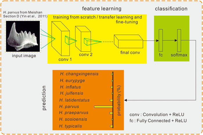
FIGURE 4. Overview of the convolutional neural network used and its procedures in the experiment. Conodont image from Yin et al. (2001).
All models were trained using an NVIDIA GeForce RTX 2070 graphics card, and the operating system version was Windows 10 Professional. Python version 3.7.0 was used, along with PyTorch version 1.10.0 and CUDA version 10.2.
After the CNN model is trained on the dataset, the next step is to evaluate the performance of the classifier obtained after training. Based on a comparison of the predicted classes on the test set and the true labels, four sets of results are obtained: the true positive sample, false positive sample, true negative sample and false negative sample. These four samples can be plotted in a confusion matrix (Figure 5) for further analysis. The confusion matrix shows the specific classification and can be used to easily calculate the values of various evaluation metrics (e.g., accuracy, precision, recall, and F1-score). These evaluation metrics can be an objective means of evaluating the generalization performance of the classifier. However, the application of these evaluation metrics is limited to balanced datasets; their application is less straightforward when the dataset is unbalanced and can even lead to incorrect evaluation results (Branco et al., 2016). Sensitivity (also called true positive rate, TPR) and specificity (also called false positive rate, FPR) are evaluation metrics that ignore the imbalance between positive and negative samples (Figure 5). Using the FPR as the horizontal coordinate and the TPR as the vertical coordinate, a receiver operating characteristic (ROC) curve can be plotted (Fawcett, 2006). When the TPR is large and the FPR is small, a steep ROC curve is obtained, indicating good performance of the classifier. The value of the area under the curve (AUC) of the ROC curve (Bradley, 1997) is usually between 0.5 and 1.0. The larger the AUC value is, the better the classifier performance. Therefore, in the case of unbalanced datasets, two metrics, ROC and AUC, are usually used instead of accuracy (Branco et al., 2016).
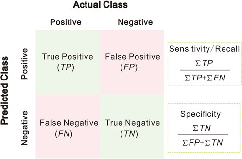
FIGURE 5. Confusion matrix and other evaluation metrics calculated from it.
The five fine-grained CNN models selected for the experiments were trained on the conodont dataset using different training strategies and hyperparameters. All models were trained with the batch size set to 8, Adam was used as the optimizer, and each model was trained 10 times (each training round was denoted K1 to K10). The training strategies, other hyperparameter settings and training results are shown in Table 2.
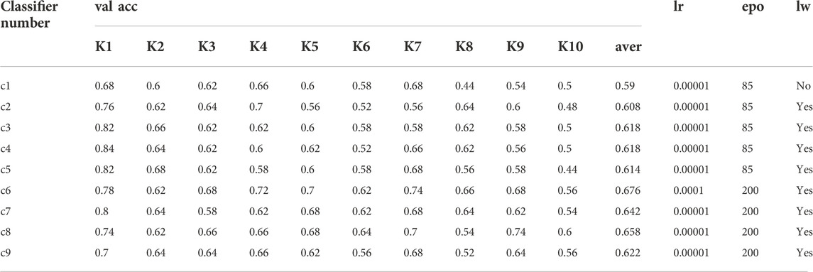
TABLE 2. Analysis of the results of seven classifications obtained by training with five fine-grained CNN models. where c1, c2, c3, c4, and c5 are the classifiers obtained after training with Bilinear-VGG16, c6 is the classifier obtained after training with Bilinear-ResNet18, c7 is the classifier obtained after training with Bilinear-ResNet50, c8 is the classifier obtained after training with CBAM-ResNet50 and c9 is the classifier obtained after training with SE-ResNet50. lr = learning rate; lw = load weights; epo = epochs.
Where c1, c2, c3, c4, and c5 are the classifiers obtained after training with Bilinear-VGG16, c6 is the classifier obtained after training with Bilinear-ResNet18, c7 is the classifier obtained after training with Bilinear-ResNet50, c8 is the classifier obtained after training with CBAM-ResNet50 and c9 classifier obtained after training with SE-ResNet50. lr = learning-rate; lw = load-weights; epo = epochs.
The bilinear VGG16 model was trained in three different ways, with a learning rate set to 0.00001 and 85 iterations per round, and the resulting classifiers were as follows: 1) in c1, pretrained weights were not trained on ImageNet and the data were trained from scratch and after 10 rounds of training, the accuracy of the classifier on the validation set ranged from 0.44 to 0.68 with a mean value of 0.59; 2) c2 uses pretrained weights and freezes the first seven convolutional layers, and the accuracy of the classifier on the validation set ranged from 0.48 to 0.76 with a mean value of 0.608; 3) c3 also freezes the first seven convolutional layers, but the network model can not only advance the texture features, but also better extract the shape features (Geirhos et al., 2019), and the accuracy of the classifier on the validation set ranged from 0.5 to 0.82 with a mean value of 0.618; 4) c4 used pretrained weights, but only the first 26 layers were frozen (i.e., the last convolutional and fully connected layers were trained), and the accuracy of the classifier on the validation set ranged from 0.5 to 0.84 with a mean value of 0.618; 5) c5 used pretrained weights, all convolutional layers were frozen, only the fully connected layers were trained, and the accuracy of the classifier on the validation set ranged from 0.44 to 0.82, with an average value of 0.614.
Using Bililinear-ResNet18 (c6) with pretraining weights loaded and all convolutional layers frozen, only the fully connected layers were trained, the learning rate was set to 0.0001 and 200 iterations per round, and the accuracy of the classifier on the validation set ranged from 0.56 to 0.78 with an average value of 0.676.
Using Bilinear-ResNe50 (c7) training with pretraining weights loaded and all convolutional layers frozen, only fully connected layers were trained with a learning rate set to 0.00001 and 200 iterations per round. The accuracy of the classifier on the validation set ranged from 0.54 to 0.8 with a mean value of 0.642.
Using CBAM-ResNet50 (c8) training with pretraining weights loaded and all convolutional layers frozen, only the fully connected layers were trained with a learning rate set to 0.00001 and 200 iterations per round. The accuracy of the classifier on the validation set ranged from 0.54 to 0.74 with a mean value of 0.658.
Using SE-ResNet50 (c9) training with pretrained weights loaded and all convolutional layers frozen and only fully connected layers trained with a learning rate set to 0.00001 and 200 iterations per round, the accuracy of the classifier on the validation set ranged from 0.52 to 0.7 with an average value of 0.622.
Comparing the average accuracy of the above seven classifiers on the validation set, the results showed that c6 had the highest average accuracy, followed by c8, and that c1 has the lowest accuracy, indicating that Bilinear-ResNet18 was the optimal model for the conodont dataset.
After determining the best model, the Bilinear-ResNet18 model was used to retrain all the data in the training dataset and to evaluate the final generated classifier.
The confusion matrix was generated using the prediction results of the classifier on the test set (Figure 6). From the prediction results, only two of the seven samples labeled H. changxingensis were correctly identified, and the other five were predicted to be H. eurypyge, H. julfensis, H. parvus, H. praeparvus, and H. typicalis, with an accuracy of 0.28. Of the six samples labeled H. eurypyge, five were correctly identified, and only one was predicted to be H. praeparvus with an accuracy of 0.83. Of the four samples labeled H. inflatus, two were correctly identified, and the remaining two were predicted to be H. julfensis with an accuracy of 0.5. Of the four samples labeled H. julfensis, three were correctly identified, and the remaining sample was predicted to be H. praeparvus with an accuracy of 0.75. Of the seven samples labeled H. latidentatus, three were correctly identified, one was predicted to be H. eurypyge, one was predicted to be H. julfensis, and the other two were predicted to be H. parvus, with an accuracy of 0.43. Of the 21 samples labeled H. parvus, 16 were correctly identified, one was predicted to be H. eurypyge, and the other four were predicted to be H. praeparvus with an accuracy of 0.76. Of the 16 samples labeled H. praeparvus, 9 were accurately identified, 2 were predicted to be H. changxingensis, 2 were predicted to be H. eurypyge, 2 were predicted to be H. latidentatus, and 1 was predicted to be H. typicalis with an accuracy of 0.56. Of the 2 samples labeled H. sosioensis, 1 was accurately identified, and 1 was predicted to be H. typicalis with an accuracy of 0.56. Of the 10 samples labeled H. typicalis, 5 were correctly identified, 3 were predicted as H. changxingensis, H. eurypyge, and H. julfensis, and 2 were predicted as H. praeparvus, with an accuracy of 0.5. Overall, the classifier was accurate on the test set. Overall, the accuracy of the classifier on the test set was 0.6.
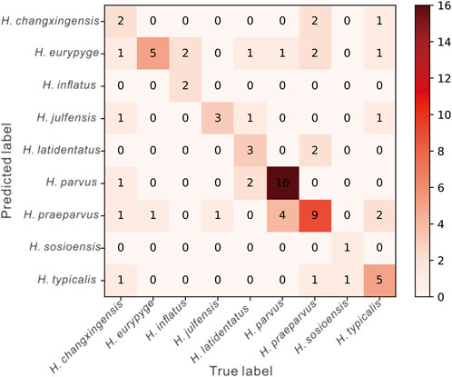
FIGURE 6. The confusion matrix is generated based on the prediction results of the final classifier on the test dataset.
Based on the confusion matrix (Figure 6), the values of sensitivity and specificity of each class can be calculated separately so that the corresponding ROC curves can be plotted and the corresponding AUC can be obtained. Hindeodus changxingensis, H. eurypyge, H. inflatus, H. julfensis, H. latidentatus, H. parvus, H. praeparvus, H. sosioensis, and H. typicalis had AUC values of 0.84, 0.94, 0.98, 0.89, 0.94, 0.92, 0.78, 0.97, and 0.84, respectively (Figure 7). The macroaverage AUC value for the classifier on the test dataset was 0.90.
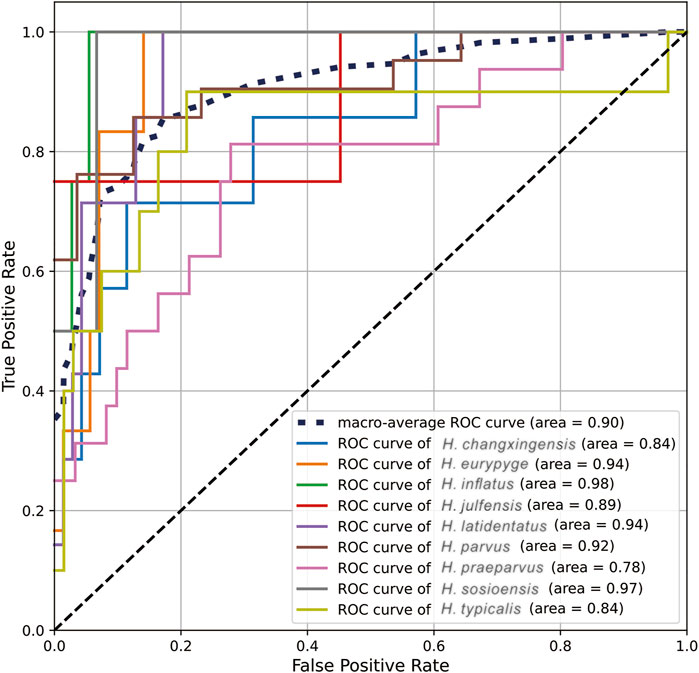
FIGURE 7. The ROC curves are generated based on the prediction results of the final classifier on the Test set.
Comparing the average accuracy of the three classifiers c1, c2, c3, c4, and c5 (Table 2), we found that loading pretraining weights and freezing all layers for training improved the performance of the model when using the same CNN model. Compared with c2, in the training process of c3, we let CNN extract more shape features, but the performance of the two classifiers is not much different. Our analysis may be due to the fact that unlike common images (such as cats, dogs, cars, etc.), almost none of the conodont fossils have strict integrity and are more or less damaged, thus leading to not very good results even though we let the network focus more on the extraction of shape features.
Both c6 and c7 are classifiers generated using the bilinear algorithm; the difference between them is that the backbone used in c6 and c7 are ResNet18 and ResNet50, respectively. The average accuracy of c6 was greater than that of c7 (Table 2), indicating that increasing the depth of the CNN did not improve the model performance. This result may be due to the simple image features of the conodonts (Liu et al., 2020); increasing the depth of the network does not necessarily result in accuracy improvement. Additionally, c7, c8, and c9 are all classifiers trained with ResNet50 as the backbone, and the average accuracy of c7, c8, and c9 on the validation set in descending order was as follows (Table 2): c8, c7, and c9. This indicated that the SE algorithm was more suitable for the conodont dataset.
The optimal classifier, c6, obtained an AUC value of 0.9 on the test set. This was a good result for the classification of a conodont species, especially considering that the model was trained in the low data regime, and some conodont images have natural defects (e.g., some parts of the fossil were missing and the surface of the fossil was covered by colloid).
As mentioned previously, the dataset in this paper had many problems that cannot be solved at this time, such as small sample size and imbalance, and these problems will likely be faced in other fields (Mikołajczyk and Grochowski, 2018). There were some conodonts in our dataset that were not well preserved during the deposition process (Figure 8A), and although experts can identify them based on their accumulated experience, identification of the samples is difficult for the machine. When using SEM to obtain images of the conodont, colloid must be used to fix the samples, which may cause the conodont surface to be attached by colloid during this process (Figure 8B). Studies have shown that CNNs rely more on texture features to identify objects compared to features such as shape and color (Shi et al., 2020), and the attached colloid alters the original texture of the conodont, making intelligent recognition of conodonts more challenging.
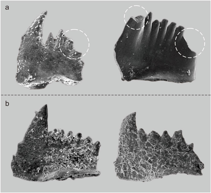
FIGURE 8. Some incomplete fossil samples [(A), the part enclosed by the white oval dotted line] and samples with surfaces attached to colloids (B).
In addition, random neighborhood embedding with t distribution (t-SNE), a tool for visualizing high-dimensional data, was used to analyze the similarity of features between conodont data. The basic principle of t-SNE is to map each data point to a corresponding probability distribution through a transformation using a Gaussian distribution to convert distances to probability distributions in high-dimensional space and a t-distribution to convert distances to probability distributions in a low-dimensional (two- or three-dimensional) space (Van der Maaten and Hinton, 2008). After t-SNE processing of the raw conodont data, we found that all categories are largely clustered together (Figure 9A). Boytsov et al. (2017) performed a clustering analysis on the raw data of the MNIST dataset (a handwritten digit dataset) using t-SNE, and the categories in the dataset were well distinguished. These two distinct results are due to the fact that conodont image data are more similar and thus not easily distinguishable; thus, the task of classifying conodont species is more difficult, while the task of distinguishing handwritten digits is less difficult. Using the same method, after training on the raw data and then processing the last layer of features with t-SNE, we found that there were obvious boundaries that could be well distinguished (Figure 9B), indicating that the classifier obtained after training was feasible. Some samples were clustered together (black dashed ellipse box in Figure 9B), indicating that these samples were difficult to identify accurately and that many species are indistinguishable from H. eurypyge, which was consistent with the results shown by the confusion matrix (Figure 6). In terms of the evolutionary lineage of Hindeodus, H. parvus is closer to H. latidentatus and H. preparvus than to H. typicalis (Wang, 1996; Lai, 1998; Perri and Farabegoli, 2003), and therefore these three species (i.e., H. parvus, H. latidentatus, and H. preparvus) can be seen to have misclassified samples from each other on the t-SNE plot (Figure 9B). H. changxingensis and H. typicalis did not evolve from H. preparvus (Perri and Farabegoli, 2003); they have a separate evolutionary lineage and therefore have little intersection with H. parvus, H. latidentatus, and H. preparvus. Studies have shown that H. sosioensis and H. anterodentatus, and H. julfensis and Isarcicella changxingensis, are the closest in affinity (Perri and Farabegoli, 2003; Jiang et al., 2014), so they can be well distinguished from other species. In addition, even two species that are very distantly related appear to be intermixed, and we speculate that the fact that the fossils are not complete causes the machine to think they are similar.
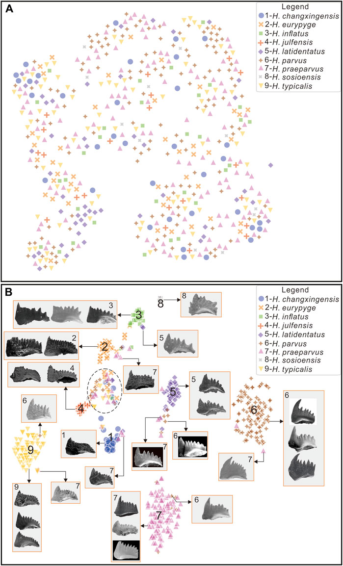
FIGURE 9. Data features visualized by t-SNE (A), visualize original data features; (B), visualize the last layer of features after training on the original data.
In general, the intelligent recognition of conodont species had several challenges: 1) the dataset was small and unbalanced; 2) some conodonts were incomplete, and this natural defect was not found in common datasets; and 3) the original textures of some conodont were damaged during the experimental process, leading them to be missing some key features. These issues resulted in the difficulty of intelligent recognition for conodonts at this stage.
To address the above problems, future work can focus on the following two aspects. The first task will be to augment the data of conodonts already collected and to collect other conodonts of the genus Hindeodus that were not included in this study (e.g., H. anterodentatus, H. bicuspidatus, H. lobatus, H. magnus, and H. priscus). The success of deep learning models in the field of computer vision has largely been attributed to large-scale labeled data (Sun et al., 2017). When recognizing images, since machines do not have prior knowledge like people, it is necessary to provide a large amount of data to the CNN for feature learning. The process of obtaining conodont image data includes extracting conodonts from sedimentary rocks and imaging them under SEM, which is a time-consuming and tedious task. To construct a dataset of conodonts including various species and large numbers requires the joint efforts of a large number of geologists. Establishing a public web platform for collecting and presenting conodont data and making it available for further study would be helpful. Second, low-quality data needs to be preprocessed. Low-quality data resulted mainly from incomplete conodonts and corrupted original textures, seriously affecting the performance of the classifier, but it was clearly not wise to discard these low-quality data when the dataset was already small. Before training the dataset, high-quality data can be formed by image restoration (e.g., recovering missing parts and texture restoration) of these low-quality data. Image restoration is the task of filling missing pixels in an image to make the finished image look realistic and suit the real-world context (Yu et al., 2019). Deep learning-based image restoration techniques have achieved good results on conventional images (e.g., faces, buildings) (Iizuka et al., 2017; Liu et al., 2018; Yu et al., 2019), and although it is not known whether these models will achieve the same results for conodont restoration, it is still worthwhile to investigate them.
In this paper, we aimed to perform intelligent identification of conodont species of the same genus to better serve geoscience research. For any automatic identification of fossils, the fossil species trained on the CNN model should belong to the same genus so that the difficulties in fossil identification work can be addressed.
In this study, we used five fine-grained CNN models to train nine species of the conodont genus Hindeodus with different strategies to obtain seven classifiers. By comparing the accuracy of these classifiers on the validation dataset, we found that the classifier trained by Bilinear-ResNet18 has the highest accuracy. We also found that increasing the number of network layers did not significantly improve the accuracy, while using transfer learning was effective. The performance of the classifier obtained by retraining all the data on the training set using Bilinear-ResNet18 was evaluated, and the AUC value of the classifier was 0.9, indicating that the final classifier was satisfactory despite some deficiencies in the dataset.
Although previous findings suggested that CNN models can be better applied for intelligent identification of paleontological fossils, we suggest that the dataset for model training be fine-grained, which is also more in line with the practical needs of fossil identification. In the future, we believe that as more and more high-quality fossil data are made available and shared, intelligent identification using CNN models will achieve better and better results, thus effectively pushing the identification of fossils in the direction of artificial intelligence.
The datasets presented in this study can be found in online repositories. The names of the repository/repositories and accession number(s) can be found below: https://www.scidb.cn/s/RbeqIj.
All the work was done by XD.
This study was funded by Natural Science Foundation of Sichuan Province (No. 2022NSFSC1177) and Fundamental Research Funds of China West Normal University (20E031).
We thank Ping Xian and Xinyi Wen of China West Normal University for checking the conodont labels. We also thank AJE (American Journal Experts) for its linguistic assistance during the preparation of this manuscript.
The authors declare that the research was conducted in the absence of any commercial or financial relationships that could be construed as a potential conflict of interest.
All claims expressed in this article are solely those of the authors and do not necessarily represent those of their affiliated organizations, or those of the publisher, the editors and the reviewers. Any product that may be evaluated in this article, or claim that may be made by its manufacturer, is not guaranteed or endorsed by the publisher.
AUC, Area Under Curve; CNN, Convolutional Neural Network; CBAM, Convolutional Block Attention Module; FPR, false positive rate; ROC, Receiver Operating Characteristic; SE, Squeeze and Excitation; SEM, Scanning Electron Microscope; TPR, true positive rate.
Arefifard, S., and Payne, J. L. (2020). End-Guadalupian extinction of larger fusulinids in central Iran and implications for the global biotic crisis. Palaeogeography, Palaeoclimatology, Palaeoecology 550, 109743. doi:10.1016/j.palaeo.2020.109743
Alférez, G. H., Vázquez, E. L., Ardila, A. M. M., and Clausen, B. L. (2021). Automatic classification of plutonic rocks with deep learning. Appl. Comput. Geosciences 10, 100061. doi:10.1016/j.acags.2021.100061
An, Y., Chen, Y., Huang, Y., Li, P., Jiang, Y., and Wang, Z. (2022). Hierarchical recognition of ostracod fossils based on deep learning. Geol. Rev. 68 (2), 673–684. (In Chinese with English abstract). doi:10.16509/j.georeview.2021.11.031
Baraboshkin, E. E., Ismailova, L. S., Orlov, D. M., Zhukovskaya, E. A., Kalmykov, G. A., Khotylev, O. V., et al. (2020). Deep convolutions for in-depth automated rock typing. Comput. Geosciences 135, 104330. doi:10.1016/j.cageo.2019.104330
Bourel, B., Marchant, R., de Garidel-Thoron, T., Tetard, M., Barboni, D., Gally, Y., et al. (2020). Automated recognition by multiple convolutional neural networks of modern, fossil, intact and damaged pollen grains. Comput. Geosciences 140, 104498. doi:10.1016/j.cageo.2020.104498
Boytsov, A., Fouquet, F., Hartmann, T., and LeTraon, Y. (2017). Visualizing and exploring dynamic high-dimensional datasets with LION-tSNE. arXiv preprint. doi:10.48550/arXiv.1708.04983
Bradley, A. P. (1997). The use of the area under the ROC curve in the evaluation of machine learning algorithms. Pattern Recognit. 30 (7), 1145–1159. doi:10.1016/S0031-3203(96)00142-2
Branco, P., Torgo, L., and Ribeiro, R. P. (2016). A survey of predictive modeling on imbalanced domains. ACM Comput. Surv. 49 (2), 1–50. doi:10.1145/2907070
Branson, S., Horn, G., Belongie, S., and Perona, P. (2014). “Bird species categorization using pose normalized deep convolutional nets,” in BMVC 2014 - proceedings of the British machine vision conference 2014 (University of Nottingham, Nottingham: BMVA Press).
Casasent, D., and Wang, Y.-C. (2005). A hierarchical classifier using new support vector machines for automatic target recognition. Neural Netw. 18 (5-6), 541–548. doi:10.1016/j.neunet.2005.06.033
de Lima, R. P., Bonar, A., Coronado, D. D., Marfurt, K., and Nicholson, C. (2019). Deep convolutional neural networks as a geological image classification tool. Sediment. Rec. 17 (2), 4–9. doi:10.2110/sedred.2019.2.4
de Vel, O., and Aeberhard, S. (2000). Object recognition using random image-lines. Image Vis. Comput. 18 (3), 193–198. doi:10.1016/s0262-8856(99)00016-5
Donahue, J., Jia, Y., Vinyals, O., Hoffman, J., Zhang, N., Tzeng, E., et al. (2014). “DeCAF: A deep convolutional activation feature for generic visual recognition,” in lnternational conference on machine learning (Beijing, China: PMLR).
Dong, J.-X., Krzyżak, A., and Suen, C. Y. (2002). Local learning framework for handwritten character recognition. Eng. Appl. Artif. Intell. 15 (2), 151–159. doi:10.1016/s0952-1976(02)00024-6
Du, Y., and Tong, J. (2009). Introduction to Palaeontology and historical geology. 2nd edition. China, Wuhan: China University of Geosciences Press. (In Chinese).
Epstein, A. G., Epstein, J. B., and Harris, L. D. (1977). Conodont color alteration; an index to organic metamorphism. Washington, DC: United States: US Government Printing Office.
Fawcett, T. (2006). An introduction to ROC analysis. Pattern Recognit. Lett. 27 (8), 861–874. doi:10.1016/j.patrec.2005.10.010
Gao, Y., Beijbom, O., Zhang, N., and Darrell, T. (2016). “Compact bilinear pooling,” in Proceedings of the IEEE conference on computer vision and pattern recognition (CVPR) (Las Vegas, NV: IEEE).
Geirhos, R., Rubisch, P., Michaelis, C., Bethge, M., Wichmann, F. A., and Brendel, W. (2019). “ImageNet-trained CNNs are biased towards texture; increasing shape bias improves accuracy and robustness,” in 7th international conference on learning representations, ICLR 2019 (New Orleans, LA: OpenReview).
Guo, Y., Zhou, Z., Lin, H., Liu, X., Chen, D., Zhu, J., et al. (2020). The mineral intelligence identification method based on deep learning algorithms. Earth Sci. Front. 27 (5), 39–47. doi:10.13745/j.esf.sf.2020.5.45
He, K., Zhang, X., Ren, S., and Sun, J. (2016). “Deep residual learning for image recognition,” in Proceedings of the IEEE conference on computer vision and pattern recognition (Las Vegas, NV: IEEE).
Hinton, G., Srivastava, N., Krizhevsky, A., Sutskever, I., and Salakhutdinov, R. (2012). Improving neural networks by preventing co-adaptation of feature detectors. arXiv preprint. doi:10.48550/arXiv.1207.0580
Hsiang, A. Y., Brombacher, A., Rillo, M. C., Mleneck-Vautravers, M. J., Conn, S., Lordsmith, S., et al. (2019). Endless Forams:> 34, 000 modern planktonic foraminiferal images for taxonomic training and automated species recognition using convolutional neural networks. Paleoceanogr. Paleoclimatology 34 (7), 1157–1177. doi:10.1029/2019pa003612
Hu, J., Shen, L., Albanie, S., Sun, G., and Wu, E. (2020). Squeeze-and-Excitation networks. IEEE Trans. Pattern Anal. Mach. Intell. 42 (8), 2011–2023. doi:10.1109/TPAMI.2019.2913372
Huang, G., Liu, Z., Van Der Maaten, L., and Weinberger, K. Q. (2017). “Densely connected convolutional networks,” in Proceedings of the IEEE conference on computer vision and pattern recognition (Honolulu, Hawaii: IEEE).
Iizuka, S., Simo-Serra, E., and Ishikawa, H. (2017). Globally and locally consistent image completion. ACM Trans. Graph. 36 (4), 1–14. doi:10.1145/3072959.3073659
Inglada, J. (2007). Automatic recognition of man-made objects in high resolution optical remote sensing images by SVM classification of geometric image features. ISPRS J. Photogramm. Remote Sens. 62 (3), 236–248. doi:10.1016/j.isprsjprs.2007.05.011
Jiang, H., Lai, X., Sun, Y., Wignall, P. B., Liu, J., and Yan, C. (2014). Permian-Triassic conodonts from Dajiang (Guizhou, South China) and their implication for the age of microbialite deposition in the aftermath of the End-Permian mass extinction. J. Earth Sci. 25 (3), 413–430. doi:10.1007/s12583-014-0444-4
Keçeli, A. S., Keçeli, S. U., and Kaya, A. (2018). “Classification of radiolarian fossil images with deep learning methods,” in 2018 26th signal processing and communications applications conference (SIU) (Izmir, Turkey: IEEE).
Khan, S. D., and Ullah, H. (2019). A survey of advances in vision-based vehicle re-identification. Comput. Vis. Image Underst. 182, 50–63. doi:10.1016/j.cviu.2019.03.001
Kotropoulos, C., and Pitas, I. (2003). Segmentation of ultrasonic images using support vector machines. Pattern Recognit. Lett. 24 (4-5), 715–727. doi:10.1016/s0167-8655(02)00177-0
Krizhevsky, A., Sutskever, I., and Hinton, G. E. (2012). ImageNet classification with deep convolutional neural networks. Commun. ACM. 60, 84–90. doi:10.1145/3065386
LeCun, Y., Bengio, Y., and Hinton, G. (2015). Deep learning. Nature 521 (7553), 436–444. doi:10.1038/nature14539
Li, S., Chen, J., and Xiang, J. (2020). Applications of deep convolutional neural networks in prospecting prediction based on two-dimensional geological big data. Neural comput. Appl. 32 (7), 2037–2053. doi:10.1007/s00521-019-04341-3
Li, T., Zuo, R., Xiong, Y., and Peng, Y. (2021). Random-drop data augmentation of deep convolutional neural network for mineral prospectivity mapping. Nat. Resour. Res. 30 (1), 27–38. doi:10.1007/s11053-020-09742-z
Lin, T.-Y., and Maji, S. (2017). “Improved bilinear pooling with CNNs,” in British machine vision conference (BMVC) (London, UK: BMVA Press).
Lin, T. Y., Roychowdhury, A., and Maji, S. (2015). “Bilinear CNN models for fine-grained visual recognition,” in Proceedings of the IEEE international conference on computer vision (Santiago, Chile: IEEE).
Liu, G., Reda, F. A., Shih, K. J., Wang, T.-C., Tao, A., and Catanzaro, B. (2018). “Image inpainting for irregular holes using partial convolutions,” in Proceedings of the European conference on computer vision (ECCV) (Munich, Germany: Springer).
Liu, T.-Z., Chen, X., Li, X., Fan, R., Liu, Y.-P., and Huan-Jin, L. (2020). Conodont image recognition based on transfer learning of deep residual neural network. Acta Palaeontol. Sin. 59 (4), 512–523. (In Chinese with English abstract). doi:10.19800/j.cnki.aps.2020.042
Liu, X., Jiang, S., Wu, R., Shu, W., Hou, J., Sun, Y., et al. (2022). Automatic taxonomic identification based on the Fossil Image Dataset (> 415, 000 images) and deep convolutional neural networks. Paleobiology, 1–22. doi:10.1017/pab.2022.14
Liu, X., and Song, H. (2020). Automatic identification of fossils and abiotic grains during carbonate microfacies analysis using deep convolutional neural networks. Sediment. Geol. 410, 105790. doi:10.1016/j.sedgeo.2020.105790
Long, J., Shelhamer, E., and Darrell, T. (2015). “Fully convolutional networks for semantic segmentation,” in Proceedings of the IEEE conference on computer vision and pattern recognition (Boston, MA: IEEE).
Long, X., Cleveland, L., and Yao, Y. L. (2006). Automatic detection of unstained viable cells in bright field images using a support vector machine with an improved training procedure. Comput. Biol. Med. 36 (4), 339–362. doi:10.1016/j.compbiomed.2004.12.002
Luo, J., and Wu, J. (2017). A survey on fine-grained image categorization using deep convolutional features. Acta Autom. Sin. 43 (8), 1306–1318. (In Chinese with English abstract). doi:10.16383/j.aas.2017.c160425
Marchant, R., Tetard, M., Pratiwi, A., Adebayo, M., and de Garidel-Thoron, T. (2020). Automated analysis of foraminifera fossil records by image classification using a convolutional neural network. J. Micropalaeontol. 39 (2), 183–202. doi:10.5194/jm-39-183-2020
Mikołajczyk, A., and Grochowski, M. (2018). “Data augmentation for improving deep learning in image classification problem,” in 2018 International interdisciplinary PhD workshop (IIPhDW) (Świnoujście, Poland: IEEE).
Minhas, R., Mohammed, A. A., and Wu, Q. J. (2010). A fast recognition framework based on extreme learning machine using hybrid object information. Neurocomputing 73 (10-12), 1831–1839. doi:10.1016/j.neucom.2009.11.049
Mitra, R., Marchitto, T., Ge, Q., Zhong, B., Kanakiya, B., Cook, M., et al. (2019). Automated species-level identification of planktic foraminifera using convolutional neural networks, with comparison to human performance. Mar. Micropaleontol. 147, 16–24. doi:10.1016/j.marmicro.2019.01.005
Mohammed, A. A., Minhas, R., Wu, Q. J., and Sid-Ahmed, M. A. (2011). Human face recognition based on multidimensional PCA and extreme learning machine. Pattern Recognit. DAGM. 44 (10-11), 2588–2597. doi:10.1016/j.patcog.2011.03.013
Ng, J., and Gong, S. (2002). Composite support vector machines for detection of faces across views and pose estimation. Image Vis. Comput. 20 (5-6), 359–368. doi:10.1016/s0262-8856(02)00008-2
Perri, M. C., and Farabegoli, E. (2003). Conodonts across the permian–triassic boundary in the Southern Alps. Cour. Forschungsinstitut Senckenberg 245, 281–313.
Pires de Lima, R., Welch, K. F., Barrick, J. E., Marfurt, K. J., Burkhalter, R., Cassel, M., et al. (2020). Convolutional neural networks as an aid to biostratigraphy and micropaleontology: A test on late paleozoic microfossils. Palaios 35 (9), 391–402. doi:10.2110/palo.2019.102
Romero, I. C., Kong, S., Fowlkes, C. C., Jaramillo, C., Urban, M. A., Oboh-Ikuenobe, F., et al. (2020). Improving the taxonomy of fossil pollen using convolutional neural networks and superresolution microscopy. Proc. Natl. Acad. Sci. U. S. A. 117 (45), 28496–28505. doi:10.1073/pnas.2007324117
Ronneberger, O., Fischer, P., and Brox, T. (2015). “U-net: Convolutional networks for biomedical image segmentation,” in 18th International conference on medical image computing and computer-assisted intervention (Munich, Germany: Springer).
Ryu, Y.-S., and Oh, S.-Y. (2001). Automatic extraction of eye and mouth fields from a face image using eigenfeatures and multilayer perceptrons. Pattern Recognit. DAGM. 34 (12), 2459–2466. doi:10.1016/s0031-3203(00)00173-4
Shen, S., and Liu, Y. (2008). Efficient multiple faces tracking based on Relevance Vector Machine and Boosting learning. J. Vis. Commun. Image Represent. 19 (6), 382–391. doi:10.1016/j.jvcir.2008.06.005
Shi, Z., Preto, N., Jiang, H., Krystyn, L., Zhang, Y., Ogg, J. G., et al. (2017). Demise of late triassic sponge mounds along the northwestern margin of the Yangtze Block, South China: Related to the carnian pluvial phase?. Palaeogeography, Palaeoclimatology, Palaeoecology 474, 247–263. doi:10.1016/j.palaeo.2016.10.031
Shi, B., Zhang, D., Dai, Q., Zhu, Z., Mu, Y., and Wang, J. (2020). “Informative dropout for robust representation learning: A shape-bias perspective,” in International conference on machine Learning, (Online: PMLR).
Simon, M., and Rodner, E. (2015). “Neural activation constellations: Unsupervised part model discovery with convolutional networks,” in Proceedings of the IEEE International conference on computer vision (ICCV) (Santiago, Chile: IEEE).
Simonyan, K., and Zisserman, A. (2015). “Very deep convolutional networks for large-scale image recognition,” in 3rd International conference on learning representations, ICLR 2015 (San Diego, CA: DBLP).
Sinha, P. (1998). A symmetry perceiving adaptive neural network and facial image recognition. Forensic Sci. Int. 98 (1-2), 67–89. doi:10.1016/s0379-0738(98)00137-6
Sun, C., Shrivastava, A., Singh, S., and Gupta, A. (2017). “Revisiting unreasonable effectiveness of data in deep learning era,” in Proceedings of the IEEE international conference on computer vision (ICCV) (Venice, Italy: IEEE).
Suresh, S., Babu, R. V., and Kim, H. J. (2009). No-reference image quality assessment using modified extreme learning machine classifier. Appl. Soft Comput. 9 (2), 541–552. doi:10.1016/j.asoc.2008.07.005
Szegedy, C., Liu, W., Jia, Y., Sermanet, P., Reed, S., Anguelov, D., et al. (2015). “Going deeper with convolutions,” in Proceedings of the IEEE conference on computer vision and pattern recognition (Boston, MA: IEEE).
Van der Maaten, L., and Hinton, G. (2008). Visualizing data using t-SNE. J. Mach. Learn. Res. 9 (11), 2579–2605.
Van Horn, G., Cole, E., Beery, S., Wilber, K., Belongie, S., and Mac Aodha, O. (2021). “Benchmarking representation learning for natural world image collections,” in Proceedings of the IEEE/CVF conference on computer vision and pattern recognition (Online: IEEE).
Wang, C. (1996). Conodont evolutionary lineage and zonation for the latest permian and the earliest triassic. Permophiles 26, 30–37.
Wang, H., Li, C., Zhang, Z., Kershaw, S., Holmer, L. E., Zhang, Y., et al. (2022). Fossil brachiopod identification using a new deep convolutional neural network. Gondwana Res. 105, 290–298. doi:10.1016/j.gr.2021.09.011
Wei, X.-S., Cui, Q., Yang, L., Wang, P., Liu, L., and Yang, J. (2022b). RPC: A large-scale and fine-grained retail product checkout dataset. Science China Information Sciences 65 (1674-733X), 197101. doi:10.1007/s11432-022-3513-y
Wei, X.-S., Xie, C.-W., Wu, J., and Shen, C. (2018). Mask-CNN: Localizing parts and selecting descriptors for fine-grained bird species categorization. Pattern Recognit. 76, 704–714. doi:10.1016/j.patcog.2017.10.002
Wei, X. S., Song, Y. Z., Mac Aodha, O., Wu, J., Peng, Y., Tang, J., et al. (2022a). “Fine-grained image analysis with deep learning: A survey,” in IEEE transactions on pattern analysis and machine intelligence 44, 8927–8948. doi:10.1109/TPAMI.2021.3126648
Woo, S., Park, J., Lee, J.-Y., and Kweon, I. S. (2018). “CBAM: Convolutional block attention module,” in Proceedings of the European conference on computer vision (ECCV) (Munich, Germany: Springer).
Xiao, T., Xu, Y., Yang, K., Zhang, J., Peng, Y., and Zhang, Z. (2015). “The application of two-level attention models in deep convolutional neural network for fine-grained image classification,” in Proceedings of the IEEE conference on computer vision and pattern recognition (Boston, MA: IEEE).
Xu, S., and Zhou, Y. (2018). Artificial intelligence identification of ore minerals under microscope based on deep learning algorithm. Acta Petrol. Sin. 34 (11), 3244–3252.
Yin, H., Zhang, K., Tong, J., Yang, Z., and Wu, S. (2001). The global stratotype section and point (GSSP) of the permian-triassic boundary. Episodes 24 (2), 102–114. doi:10.18814/epiiugs/2001/v24i2/004
Yu, J., Lin, Z., Yang, J., Shen, X., Lu, X., and Huang, T. S. (2019). “Free-form image inpainting with gated convolution,” in 2019 IEEE/CVF International Conference on Computer Vision (ICCV), 4470–4479.
Yuan, D., and Shen, S. (2011). Conodont succession across the Permian-Triassic boundary of the Liangfengya section, Chongqing, South China. Acta Palaeontologica Sinica 50 (4), 420–438. (In Chinese with English abstract). doi:10.19800/j.cnki.aps.2011.04.002
Zhang, N., Donahue, J., Girshick, R., and Darrell, T. (2014). “Part-based R-CNNs for fine-grained category detection,” in Computer vision – ECCV 2014. Editors D. Fleet, T. Pajdla, B. Schiele, and T. Tuytelaars (Springer International Publishing), 834–849.
Zhang, Y., Li, M., and Han, S. (2018). Automatic identification and classification in lithology based on deep learning in rock images. Acta Petrol. Sin. 34 (2), 333–342. (In Chinese).
Keywords: conodont, CNN, fine-grained, hindeodus, transfer learning
Citation: Duan X (2023) Automatic identification of conodont species using fine-grained convolutional neural networks. Front. Earth Sci. 10:1046327. doi: 10.3389/feart.2022.1046327
Received: 16 September 2022; Accepted: 08 November 2022;
Published: 12 January 2023.
Edited by:
Olev Vinn, University of Tartu, EstoniaReviewed by:
Haijun Song, China University of Geosciences Wuhan, ChinaCopyright © 2023 Duan. This is an open-access article distributed under the terms of the Creative Commons Attribution License (CC BY). The use, distribution or reproduction in other forums is permitted, provided the original author(s) and the copyright owner(s) are credited and that the original publication in this journal is cited, in accordance with accepted academic practice. No use, distribution or reproduction is permitted which does not comply with these terms.
*Correspondence: Xiong Duan, ZHVhbnhpb25nMDBAMTYzLmNvbQ==
Disclaimer: All claims expressed in this article are solely those of the authors and do not necessarily represent those of their affiliated organizations, or those of the publisher, the editors and the reviewers. Any product that may be evaluated in this article or claim that may be made by its manufacturer is not guaranteed or endorsed by the publisher.
Research integrity at Frontiers
Learn more about the work of our research integrity team to safeguard the quality of each article we publish.