Fractional laplacians viscoelastic wave equation low-rank temporal extrapolation

The fractional Laplacians constant-Q (FLCQ) viscoelastic wave equation can describe seismic wave propagation accurately in attenuating media. A staggered-grid pseudo-spectral (SGPS) method is usually applied to solve this wave equation but it is of only second-order accuracy in time, due to a second-order finite-difference (FD) time differentiation. Visible time dispersion and numerical instability could appear in the case of a large timestepping size. To resolve this problem, we develop a more accurate low-rank temporal extrapolation scheme for the FLCQ viscoelastic wave equation. We realize this goal by deriving an analytical time-marching formula from the general solution of the FLCQ wave equation. Compressional (P) and shear (S) wave velocities dependent k-space operators are involved in the formula and they can compensate for the time dispersion errors caused by the FD time differentiation. To implement the k-space operators efficiently in heterogeneous media, we adopt a low-rank approximation of these operators, which reduces the computational cost at each time step to several fast Fourier transforms (FFTs). Another benefit of the low-rank extrapolation is explicit separation of P and S waves, which is helpful for further developing vector wavefield-based seismic migration methods. Several numerical examples are presented to verify the higher accuracy and the less restrictive stability condition of the low-rank temporal extrapolation than the traditional SGPS extrapolation.

Introduction

Numerical simulation of viscoelastic wave equation is a useful tool to analyze seismic attenuation. It also plays a key forward engine in seismic imaging and inversion methods. The time-domain constant-Q (CQ) viscoelastic wave equations are preferred in the context of seismic modeling, because of their high efficiency and accuracy in simulating seismic wavefields in frequency-independent Q attenuating media (Kjartansson, 1979; Blanch et al., 1995). Among the existing CQ wave equations, the newly developed viscoacoustic/viscoelastic wave equations featuring a few fractional Laplacians have been verified highly accurate in describing seismic attenuation (Zhu and Carcione, 2014; Zhu and Harris, 2014; Yang and Zhu, 2018; Mu et al., 2022; Wang et al., 2022). This kind of CQ wave equation also brings accuracy improvements in Q-compensated reverse-time migration (Q-RTM) methods, due to approximately decoupling the amplitude loss and phase distortion operators (Zhu et al., 2014; Sun et al., 2015; Li et al., 2016; Wang Y. et al., 2018; Chen et al., 2020a). Another benefit of the FLCQ wave equations is the explicit Q term in the equations, which facilitates developing full waveform inversion methods (Chen et al., 2017; 2020b; Xing and Zhu, 2020; Yang et al., 2020; Xing and Zhu, 2022).

The introduction of fractional derivatives to describe the dissipation of seismic waves is pioneered by Caputo (1967) in geophysical community. Later, Carcione et al. (2002) used a simple fractional time derivative to represent the dispersion relation of the CQ model and derived a CQ viscoacoustic wave equation in terms of a (2 − 2γ)-order time derivative (0 ≤ γ < 0.5). Considering the globality of fractional derivatives, numerical approximation of the fractional time derivative demands storing all historical wavefields in theory, which is unrealistic for large-scale problems. By contrast, the fractional spatial derivatives can be calculated conveniently in the Fourier domain and the switch from the fractional time derivatives to the fractional spatial derivatives gives rise to the FLCQ formulations (Carcione, 2010; Zhu and Harris, 2014). With the help of FFT, the computational efficiency for solving the FLCQ wave equations can be ensured. Recently, Xue et al. (2018) and Zhao et al. (2020) used a domain decomposition method to improve the computational efficiency of the FFT simulation scheme further.

A key aspect in numerical simulation of FLCQ wave equations is the treatment to the space variable-order fractional Laplacians. The space average strategy by Zhu and Harris (2014) only offers reasonable accuracy in the case of a smooth Q model but introduces large simulation errors in the case of a sharp Q variation. Several different approximations have been developed to transform the variable-order fractional Laplacians into constant-order fractional Laplacians (Chen et al., 2016; Yang and Zhu, 2018; Xing and Zhu, 2019; Mu et al., 2021), which facilitates the FFT simulations, significantly. Although the FFT differentiation achieves a spectral accuracy in space, the tradtional pseudo-spectral (PS) method uses a second-order FD operator to approximate the time derivative, which limits the temporal extrapolation accuracy to second-order. When a relatively large timestepping size is used, the traditional PS temporal extrapolation suffers from visible time dispersion and a strict Courant-Friedrichs-Lewy (CFL) stability condition. Koene et al. (2018) applied a pair of pre- and post-propagation filters to correct the time dispersion and this method almost does not introduce any computational cost. However it is only valid for elastic media, where the time dispersion is independent of the wave propagation.

Several endeavors have been done to enhance the temporal extrapolation accuracy in seismic modeling, including accurate acoustic/elastic time-marching formulae based on the formal solutions of wave equations (Etgen and Dellinger, 1989). This scheme is later generalized to anisotropic wave equations where it is reffered to as a pseudo-analytical method (Chu and Stoffa, 2010; Yan and Liu, 2016). Zhang and Zhang (2009) developed one-step temporal extrapolation schemes that are free of numerical dispersion. Pestana and Stoffa (2010) adopted the Chebyshev polynomials to approximate the cosine operator involved in an analytical time-marching formula, resulting in a highly accurate temporal extrapolation. Fomel et al. (2013) and Fang et al. (2014) presented low-rank temporal extrapolation schemes for scalar wave equation and it is later generalized to elastic wave equation (Sun et al., 2017; Huang and Liu, 2020). Although the mentioned methods improve the time approximation accuracy, they are limited to elastic media. Sun et al. (2015) and Chen et al. (2016) presented low-rank temporal extrapolation schemes for the FLCQ viscoacoustic wave equation. Recently, Chen et al. (2021) developed an efficient fourth-order PS temporal extrapolation method for viscoacoustic modeling and Q-RTM. Even so, further extension of the low-rank or the fourth-order extrapolation schemes to the FLCQ viscoelastic wave equation has not been reported.

The goal of this work is to develop an efficient low-rank temporal extrapolation scheme for the FLCQ viscoelastic wave equation to provide a highly accurate elastic modeling approach in attenuating media.

Methods

In this section, we first introduce the general solution of the CQFL viscoelastic wave equation and deduce an analytical three-step time-marching formula. Then, we reformulate the time-marching scheme into a first-order system in terms of particle velocity and stress to incorporate the well-establised perfectly matched layer (PML) as absorbing boundary conditions. Next, we introduce the principle of the low-rank approximation and evaluate the overall computational cost of the viscoelastic low-rank modeling scheme.

A general solution of viscoelastic wave equation

The isotropic FLCQ viscoelastic wave equation in terms of velocity and stress can be expressed as (Zhu and Carcione, 2014):

$\frac{\partial \mathit{\varphi }}{\partial t}=\mathit{L}\mathit{\varphi },(1)$

$\mathit{L}=\left(\begin{array}{ccccc}\hfill 0\hfill & \hfill 0\hfill & \hfill {\partial }_x\hfill & \hfill {\partial }_z\hfill & \hfill 0\hfill \\ \hfill 0\hfill & \hfill 0\hfill & \hfill 0\hfill & \hfill {\partial }_x\hfill & \hfill {\partial }_z\hfill \\ \hfill \left({\mathcal{D}}_p+{\mathcal{A}}_p\right){\partial }_x\hfill & \hfill \left[{\mathcal{D}}_p+{\mathcal{A}}_p-2\left({\mathcal{D}}_s+{\mathcal{A}}_s\right)\right]{\partial }_z\hfill & \hfill 0\hfill & \hfill 0\hfill & \hfill 0\hfill \\ \hfill \left({\mathcal{D}}_s+{\mathcal{A}}_s\right){\partial }_z\hfill & \hfill \left({\mathcal{D}}_s+{\mathcal{A}}_s\right){\partial }_x\hfill & \hfill 0\hfill & \hfill 0\hfill & \hfill 0\hfill \\ \hfill \left[{\mathcal{D}}_p+{\mathcal{A}}_p-2\left({\mathcal{D}}_s+{\mathcal{A}}_s\right)\right]{\partial }_x\hfill & \hfill \left({\mathcal{D}}_p+{\mathcal{A}}_p\right){\partial }_z\hfill & \hfill 0\hfill & \hfill 0\hfill & \hfill 0\hfill \end{array}\right),(2)$

where

$\mathit{\varphi }={\left(\rho v_x,\rho v_z,{\rho }^{-1}{\sigma }_{xx},{\rho }^{-1}{\sigma }_{xz},{\rho }^{-1}{\sigma }_{zz}\right)}^T,(3)$

${\mathcal{D}}_l={\eta }_l{\left(-{\nabla }^2\right)}^{{\gamma }_l},{\mathcal{A}}_l={\tau }_l\frac{\partial }{\partial t}{\left(-{\nabla }^2\right)}^{{\gamma }_l-\frac{1}{2}},(4)$

$\begin{array}{cc}\hfill {\eta }_l& ={\omega }_o^{-2{\gamma }_l}{c}_l^{2{\gamma }_l+2}{\cos }^2\left(\frac{\pi {\gamma }_l}{2}\right)\cos \left(\pi {\gamma }_l\right),\hfill \\ \hfill {\tau }_l& ={\omega }_o^{-2{\gamma }_l}{c}_l^{2{\gamma }_l+1}{\cos }^2\left(\frac{\pi {\gamma }_l}{2}\right)\sin \left(\pi {\gamma }_l\right),\hfill \end{array}(5)$

${\gamma }_l=\frac{1}{\pi }\arctan \left(\frac{1}{Q_l}\right),(6)$

where $l\in \left\{p,s\right\}$ denotes P- and S-wave respectively, (v_x, v_z) are particle velocities, (σ_xx, σ_xz, σ_zz) are stress components, ∂_(.) represents the first-order space derivatives, ρ is density, ω_o denotes a reference frequency where the wave speeds c_l are defined.

Eq. 1 is previously solved by a SGPS method where the spatial variable-order of the fractional Laplacian is replaced by an average value. Wang N. et al. (2018) adopted the approximation proposed by Chen et al. (2016) to transform the spatial variable-order Laplacians to fixed-order Laplacians and improved the simulation accuracy. However, the simulation scheme is only second-order accurate in time.

In this case of a homogeneous medium, Eq. 1 can be reformulated into a second-order form in terms of displacements (u, w):

$\left\{\begin{array}{c}\frac{{\partial }^{2}u}{\partial t^2}-\left({\mathcal{D}}_p+{\mathcal{A}}_p\right)\frac{{\partial }^{2}u}{\partial x^2}-\left({\mathcal{D}}_s+{\mathcal{A}}_s\right)\frac{{\partial }^{2}u}{\partial z^2}-\left({\mathcal{D}}_p+{\mathcal{A}}_p-{\mathcal{D}}_s-{\mathcal{A}}_s\right)\frac{{\partial }^{2}w}{\partial x\partial z}=0,\hfill \\ \frac{{\partial }^{2}w}{\partial t^2}-\left({\mathcal{D}}_s+{\mathcal{A}}_s\right)\frac{{\partial }^{2}w}{\partial x^2}-\left({\mathcal{D}}_p+{\mathcal{A}}_p\right)\frac{{\partial }^{2}w}{\partial z^2}-\left({\mathcal{D}}_p+{\mathcal{A}}_p-{\mathcal{D}}_s-{\mathcal{A}}_s\right)\frac{{\partial }^{2}u}{\partial x\partial z}=0.\hfill \end{array}\right.(7)$

By transforming Eq. 7 into the wavenumber domain, we obtain a second-order ordinary differential equations system (ODES):

$\frac{{\partial }^2\tilde{\mathit{U}}}{\partial t^2}+\mathit{A}\frac{\partial \tilde{\mathit{U}}}{\partial t}+\mathit{B}\tilde{\mathit{U}}=\mathbf{0},(8)$

$\mathit{A}=\mathit{e}\left[\begin{array}{cc}\hfill a_p\hfill & \hfill 0\hfill \\ \hfill 0\hfill & \hfill a_s\hfill \end{array}\right]{\mathit{e}}^T,\mathit{B}=\mathit{e}\left[\begin{array}{cc}\hfill b_p\hfill & \hfill 0\hfill \\ \hfill 0\hfill & \hfill b_s\hfill \end{array}\right]{\mathit{e}}^T,(9)$

$\mathit{e}=\frac{1}{k}\left[\begin{array}{cc}\hfill k_x\hfill & \hfill -k_z\hfill \\ \hfill k_z\hfill & \hfill k_x\hfill \end{array}\right],(10)$

where $\tilde{\mathit{U}}=\left(\tilde{u},\tilde{w}\right)$ with the tilde denoting the wavefield variables in the wavenumber domain, $\left(k_x,k_z\right)$ represents discrete wavenumbers, $k=\sqrt{k_x^2+k_z^2}$, and

$a_l={\tau }_l{k}^{2{\gamma }_l+1},b_l={\eta }_l{k}^{2{\gamma }_l+2},l\in \left\{p,s\right\}.(11)$

We derive a general solution of Eq. 8 as follows:

$\tilde{\mathit{U}}\left(t\right)=e^{-\frac{\mathit{A}}{2}t}\left[\cos \left(\mathit{H}t\right){\mathit{c}}_1+\sin \left(\mathit{H}t\right){\mathit{c}}_2\right],(12)$

where

$\mathit{H}=\frac{\sqrt{4\mathit{B}-{\mathit{A}}^2}}{2},(13)$

and c₁ and c₂ are two undetermined vectors depending on specific initial and boundary conditions. Since Eq. 12 is established with the homogeneous model parameters and ignorance of any sources, it is inapplicable for inhomogeneous media or injection of a source term. To resolve this problem, we further derive an analytical three-step time-marching formula from Eq. 12:

$e^{\frac{\mathit{A}}{2}\mathrm{\Delta }t}{\tilde{\mathit{U}}}^{n+1}+e^{-\frac{\mathit{A}}{2}\mathrm{\Delta }t}{\tilde{\mathit{U}}}^{n-1}-2\cos \left(\mathit{H}\mathrm{\Delta }t\right){\tilde{\mathit{U}}}^n=0,(14)$

where Δt represents a timestepping size and the superscripts n + 1, n, n − 1 denote three adjacent time steps. A source term can be injected into Eq. 14 and the temporal extrapolation is unconditionally stable without numerical dispersion in homogeneous media.

However, Eq. 14 is not a friendly formulation to welcome heterogeneous model parameters and any absorbing boundary conditions. Therefore, we rewrite Eq. 14 as:

$\frac{{\tilde{\mathit{U}}}^{n+1}-2{\tilde{\mathit{U}}}^n+{\tilde{\mathit{U}}}^{n-1}}{\mathrm{\Delta }{t}^2}=\frac{2e^{-\frac{\mathrm{\Delta }t}{2}\mathit{A}}}{\mathrm{\Delta }{t}^2}\left[\cos \left(\mathit{H}\mathrm{\Delta }t\right)-\frac{1}{2}\left(e^{\frac{\mathrm{\Delta }t}{2}\mathit{A}}+e^{-\frac{\mathrm{\Delta }t}{2}\mathit{A}}\right)\right]{\tilde{\mathit{U}}}^n-\frac{\mathit{I}-e^{-\mathrm{\Delta }t\mathit{A}}}{\mathrm{\Delta }t}\frac{{\tilde{\mathit{U}}}^n-{\tilde{\mathit{U}}}^{n-1}}{\mathrm{\Delta }t},(15)$

where I denotes an identity matrix. Considering Δt is usually small (in milliseconds), we use the following approximations:

$e^{-\frac{\mathrm{\Delta }t\mathit{A}}{2}}\approx \mathit{I}-\frac{\mathrm{\Delta }t}{2}\mathit{A},e^{-\mathrm{\Delta }t\mathit{A}}\approx \mathit{I}-\mathrm{\Delta }t\mathit{A},(16)$

to change Eq. 15 into

$\frac{{\tilde{\mathit{U}}}^{n+1}-2{\tilde{\mathit{U}}}^n+{\tilde{\mathit{U}}}^{n-1}}{\mathrm{\Delta }{t}^2}=\left(\mathit{I}-\frac{1}{2}\mathrm{\Delta }t\mathit{A}\right)\frac{2\left[\cos \left(\mathit{H}\mathrm{\Delta }t\right)-\mathit{I}\right]}{\mathrm{\Delta }{t}^2}{\tilde{\mathit{U}}}^n-\mathit{A}\frac{{\tilde{\mathit{U}}}^n-{\tilde{\mathit{U}}}^{n-1}}{\mathrm{\Delta }t}.(17)$

The subsequent numerical examples will demonstrate the negligible effects of the approximations on the simulation accuracy.

The eigenvalue decomposition of H results in

$\mathit{H}=\mathit{e}\left[\begin{array}{cc}\hfill {\beta }_p\hfill & \hfill 0\hfill \\ \hfill 0\hfill & \hfill {\beta }_s\hfill \end{array}\right]{\mathit{e}}^T,(18)$

where

${\beta }_l=\sqrt{{\eta }_l{k}^{2{\gamma }_l+2}-\frac{1}{4}{\tau }_l^2{k}^{4{\gamma }_l+2}},l\in \left\{p,s\right\}.(19)$

Based on Eq. 18, one can easily derive the detailed expression of the functional matrix,

$\cos \left(\mathit{H}\mathrm{\Delta }t\right)=\mathit{e}\left[\begin{array}{cc}\hfill \cos \left({\beta }_p\mathrm{\Delta }t\right)\hfill & \hfill 0\hfill \\ \hfill 0\hfill & \hfill \cos \left({\beta }_s\mathrm{\Delta }t\right)\hfill \end{array}\right]{\mathit{e}}^T.(20)$

By substituting Eqs. 9, 20 into Eq. 17 and introducing intermediate wavefield variables, we can transform the second-order time-marching system in Eq. 17 into an equivalent first-order time-marching system. After that, we finally transform the time-marching equation system back to the space domain, which gives.

${\partial }_t^{-}{v}_x^{n+\frac{1}{2}}={\partial }_x{P}^n+{\partial }_x{\sigma }_{xx}^n+{\partial }_z{\sigma }_{xz}^n,(\mathrm{21a})$

${\partial }_t^{-}{v}_z^{n+\frac{1}{2}}={\partial }_x{\sigma }_{xz}^n+{\partial }_z{P}^n+{\partial }_z{\sigma }_{zz}^n,(\mathrm{21b})$

${\partial }_t^{+}{\sigma }_{xx}^n=-2\left[c_s^{2+2{\gamma }_s}{\partial }_z^{\left(s\right)}{v}_z^{n+\frac{1}{2}}+{\tau }_s{\left(-{\nabla }^2\right)}^{{\gamma }_s-\frac{1}{2}}{\partial }_t^{-}{\partial }_z{v}_z^{n+\frac{1}{2}}\right],(\mathrm{21c})$

${\partial }_t^{+}{\sigma }_{zz}^n=-2\left[c_s^{2+2{\gamma }_s}{\partial }_x^{\left(s\right)}{v}_x^{n+\frac{1}{2}}+{\tau }_s{\left(-{\nabla }^2\right)}^{{\gamma }_s-\frac{1}{2}}{\partial }_t^{-}{\partial }_x{v}_x^{n+\frac{1}{2}}\right],(\mathrm{21d})$

${\partial }_t^{+}{\tilde{P}}^n=c_p^{2+2{\gamma }_p}\left({\partial }_x^{\left(p\right)}{v}_x^{n+\frac{1}{2}}+{\partial }_z^{\left(p\right)}{v}_z^{n+\frac{1}{2}}\right)+{\tau }_p{\left(-{\nabla }^2\right)}^{{\gamma }_p-\frac{1}{2}}{\partial }_t^{-}\left({\partial }_x{v}_x^{n+\frac{1}{2}}+{\partial }_z{v}_z^{n+\frac{1}{2}}\right),(21e)$

${\partial }_t^{+}{\sigma }_{xz}^n=c_s^{2+2{\gamma }_s}\left({\partial }_x^{\left(s\right)}{v}_z^{n+\frac{1}{2}}+{\partial }_z^{\left(s\right)}{v}_x^{n+\frac{1}{2}}\right)+{\tau }_s{\left(-{\nabla }^2\right)}^{{\gamma }_s-\frac{1}{2}}{\partial }_t^{-}\left({\partial }_x{v}_z^{n+\frac{1}{2}}+{\partial }_z{v}_x^{n+\frac{1}{2}}\right),(\mathrm{21f})$

Where the time differencing operators are defined as:

${\partial }_t^{+}{f}^n=\frac{f^{n+1}-f^n}{\mathrm{\Delta }t},{\partial }_t^{-}{f}^n=\frac{f^n-f^{n-1}}{\mathrm{\Delta }t},(22)$

and the Fourier responses of the pseudo-differential operators (PSDO) are defined as:

$\mathcal{F}\left({\partial }_r^{\left(l\right)}\right)=\tilde{i}{k}_r{\xi }_l,r\in \left\{x,z\right\},(23)$

${\xi }_l=\frac{2\left(1-\frac{\mathrm{\Delta }t}{2}{\tau }_l{k}^{2{\gamma }_l+1}\right)\left[1-\cos \left({\beta }_l\mathrm{\Delta }t\right)\right]}{c_l^{2+2{\gamma }_l}{k}^2\mathrm{\Delta }{t}^2},l\in \left\{p,s\right\},(24)$

where $\mathcal{F}$ denotes the forward Fourier transform and $\tilde{i}$ is the imaginary unit.

The PSDO in Eq. 24 can compensate for the errors caused by the FD approximations of the time derivatives, which produces a highly accurate temporal extrapolation. Note that ∂_x and ∂_z in Eq. 21a, Eq. 21b, Eq. 21c, Eq. 21d, Eq. 21e, Eq. 21f denote the traditional first-order derivatives and their Fourier spectra correspond to the traditional spectra (ignoring the operators ξ_l in Eq. 23). We provide the detailed derivations of Eq. 21a, Eq. 21b, Eq. 21c, Eq. 21d, Eq. 21e, Eq. 21f from Eq. 17 in the Appendix. The density can be incorporated into the time-marching equation system by multiplying the left-hand side of Eq. 21a, Eq. 21b by ρ and multiplying the left-hand side of Eq. 21c, Eq. 21d, Eq. 21e, Eq. 21f by ρ⁻¹.

Low-rank approximations to pseudo-differential operators

The Fourier spectra of PSDO in Eq. 23 involve heterogeneus model parameters η_l, τ_l and γ_l and this brings difficulty to numerical calculations of PSDO. A pointwise FFT scheme following the locality principle can be used theoretically. The computational cost is proportional to N_c,Q, where N_c,Q denotes the total number of different velocity and Q values in a specific model. Consider the model parameters could vary quickly in space, the computational cost is unaffordable. To resolve this problem, we adopt the low-rank approximation (Fomel et al., 2013) to treat the mixed-domain operators ξ_l, which keeps the numerical calculations of PSDO efficiently.

For simplicity, we ignore the subscript l and express ξ as a k-space domain matrix:

$\mathit{W}\left(\mathit{x},\mathit{k}\right)=\left\{\left.\xi \left({\mathit{x}}_i,{\mathit{k}}_j\right)\right|0\le i<N,0\le j<N\right\},(25)$

where ${\mathit{x}}_i=\left({\eta }_i,{\tau }_i,{\gamma }_i\right)$ denotes the model parameters at ith grid index of the space-domain vector x, ${\mathit{k}}_j=\sqrt{{\left({\mathit{k}}_x\right)}_j^2+{\left({\mathit{k}}_z\right)}_j^2}$ denotes the jth element of the wavenumber-domain vector k, k_x, k_z represent x- and z-axis wavenumber vectors, and N is the total number of space/wavenumber domain grid nodes. Then, we apply a low-rank decomposition to the mixed-domain matrix:

$\mathit{W}{\left(\mathit{x}\text{,\hspace{0.17em}}\mathit{k}\right)}_{N\times N}\approx {\mathit{W}}_1{\left(\mathit{x},{\mathit{k}}_m\right)}_{N\times m}{\mathit{G}}_{m\times n}{\mathit{W}}_2{\left({\mathit{x}}_n,\mathit{k}\right)}_{n\times N},(26)$

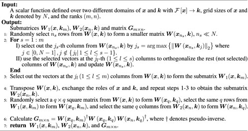
where W₁, G and W₂ are three smaller matrices with their sizes indicated in Eq. 26, m and n are refferred to as ranks. k_m is a subset of k containing m representative wavenumber elements and x_n is a subset of x containing n representative space elements. Algorithm 1 describes the low-rank decomposition process.

After the low-rank decomposition, numerical calculations of PSDO can be expressed as:

${\partial }_r^{\left(l\right)}P\left(\mathit{x}\right)\approx \sum _{j=1}^m{\mathit{W}}_1\left(\mathit{x},{\mathit{k}}_j\right){\odot }_{\mathit{x}}\sum _{i=1}^n{G}_{j,i}{\mathcal{F}}^{-1}\left\{\tilde{i}{\mathit{k}}_r{\odot }_{\mathit{k}}{\mathit{W}}_2\left({\mathit{x}}_i,\mathit{k}\right){\odot }_{\mathit{k}}\mathcal{F}\left[P\left(\mathit{x}\right)\right]\right\},(27)$

where $l\in \left\{p,s\right\}$, $r\in \left\{x,z\right\}$, ${\mathcal{F}}^{-1}$ denotes inverse FFT (IFFT) and ⊙_x, ⊙_k represent the elementwise multiplications in the space and wavenumber domains, respectively. Eq. 27 indicates that the low-rank differentiation requires one time of FFT and n times of IFFT. The actual values of n depend on the timestepping size Δt and the spatial complexity of the model parameters.

The fractional Laplacians ${\left(-{\nabla }^2\right)}^{{\gamma }_l-\frac{1}{2}}$ in Eq. 21a, Eq. 21b, Eq. 21c, Eq. 21d, Eq. 21e, Eq. 21f mainly control the amplitude loss and they can also be calculated using the low-rank approximation. However, we use a more efficient zero-order Taylor approximation to simplify the numerical calculations of these fractional Laplacians. The conducted approximations are described as follows:

$\begin{array}{ll}\hfill {\tau }_l\mathcal{F}\left[{\left(-{\nabla }^2\right)}^{{\gamma }_l-\frac{1}{2}}\right]& =c_l{\cos }^2\left(\frac{\pi {\gamma }_l}{2}\right)\sin \left(\pi {\gamma }_l\right){\left(\frac{{\omega }_d}{{\omega }_o}\right)}^{2{\gamma }_l}{k}^{-1}{\left(\frac{k}{k_{l,d}}\right)}^{2{\gamma }_l}\hfill \\ \hfill & \approx c_l{\cos }^2\left(\frac{\pi {\gamma }_l}{2}\right)\sin \left(\pi {\gamma }_l\right){\left(\frac{{\omega }_d}{{\omega }_o}\right)}^{2{\gamma }_l}{k}^{-1},\hfill \end{array}(28)$

${\tau }_l{\left(-{\nabla }^2\right)}^{{\gamma }_l-\frac{1}{2}}\approx {\tau }_l^a{\left(-{\nabla }^2\right)}^{-\frac{1}{2}},(29)$

where ω_d represents the dominant frequency of the source wavelet, k_l,d = ω_d/c_l denotes the dominant wavenumber and

${\tau }_l^a=c_l{\cos }^2\left(\frac{\pi {\gamma }_l}{2}\right)\sin \left(\pi {\gamma }_l\right){\left(\frac{{\omega }_d}{{\omega }_o}\right)}^{2{\gamma }_l}.(30)$

The zero-order Taylor approximation is feasible for three reasons: a) injection of a band-limited wavelet as the source indicates $k//k_{l,d}\approx 1$, b) 2γ_l is very closed to zero, c) the effects of the fractional orders γ_l on the amplitude loss are much weaker than the coefficients ${\tau }_l^a$.

Concluding Eq. 21a, Eq. 21b, Eq. 21c, Eq. 21d, Eq. 21e, Eq. 21f and the approximations in Eq. 29 reveals that the proposed first-order time-marching scheme requires 18 + 2n_p + 4n_s times of FFT at each time step, where n_p and n_s denote the ranks in the low-rank decompositions of P- and S-wave parameters dependent mixed-domain operators, respectively. Additionally, the computational cost of the low-rank decomposition is linear in N and it is finished before wave propagation. Thus, the cost for the low-rank decomposition in Eq. 26 is negligible.

Wang N. et al. (2018) developed a constant-order FLCQ viscoelastic wave equation that can be solved by the traditional SGPS method directly, which requires 24 times of FFT per time step. Although the low-rank temporal extrapolation usually involves more FFTs, its higher time approximation accuracy and more relaxed CFL stability condition enable a larger timestepping size for temporal extrapolation. Consequently, the low-rank modeling scheme can be more efficient than the traditional SGPS scheme, as verified by Chen et al. (2016) in FLCQ viscoacoustic modeling.

Another benefit of the time-marching scheme in Eqs. 21a, Eqs. 21b, Eqs. 21c, Eqs. 21d, Eqs. 21e, Eqs. 21f is explicit separation of P and S waves. P represents a scalar wavefield like the pressure in the acoustic wave equation and it only contains P waves. Therefore, a direct splitting of v_x and v_z as follows can generate separated P and S waves:

$\left\{\begin{array}{c}{\partial }_t^{-}{v}_{x,p}^{n+\frac{1}{2}}={\partial }_x{P}^n,v_{x,s}^{n+\frac{1}{2}}=v_x^{n+\frac{1}{2}}-v_{x,p}^{n+\frac{1}{2}},\hfill \\ {\partial }_t^{-}{v}_{z,p}^{n+\frac{1}{2}}={\partial }_z{P}^n,v_{z,s}^{n+\frac{1}{2}}=v_z^{n+\frac{1}{2}}-v_{z,p}^{n+\frac{1}{2}},\hfill \end{array}\right.(31)$

where $v_{r,p}^{n+\frac{1}{2}}$ and $v_{r,s}^{n+\frac{1}{2}},r=(x,z)$ denote the decoupled P and S wavefields, respectively. The explicit decoupling of P and S wavefields is helpful for developing elastic migration methods.

Numerical results

We use three numerical examples to demonstrate the feasibility of the viscoelastic low-rank modeling scheme. In the first example, the numerical solutions by the low-rank scheme in a homogeneous model are compared with the analytical solutions calculated by a Green function approach Carcione et al. (1988). A two-layer model with a sharp velocity contrast is then used in the second example to show the stability of the low-rank modeling scheme. Finally, a modified Marmousi-II model (Martin et al., 2006) is used to demonstrate the accuracy of the low-rank modeling scheme in complex models.

Comparison with analytical solutions

We first use the low-rank temporal extrapolation scheme to simulate wave propagation in a homogeneous model with c_p = 3 km/s, c_s = 2 km/s, Q_p = 50, ω_o = 188.50 rad/s, and Q_s = 20. The model consists of 820 × 820 grid points with the grid spacing of h = 10 m. A Ricker wavelet with the dominant frequency of 30 Hz is placed at the center of the model and is applied to v_z to mimic a vertical source. A receiver is located at (x, z) = (6110, 6110) m with an offset of 3 km. We use three different timestepping sizes of Δt = 4 ms, 2.3 ms and 2 ms for the low-rank temporal extrapolation with the same ranks of m = n = 1. Note that with such large time steps, the CFL stability condition of the traditional SGPS temporal extrapolation ($c_p\mathrm{\Delta }t/h<\sqrt{2}/\pi \approx 0.45$ in elastic media) is severely broken.

Because the low-rank temporal extrapolation scheme is derived analytically, it is highly accurate even if a large timestepping size is used, as shown in Figure 1, where the low-rank solutions match the analytical solutions well. The low-rank solutions only exhibit slight errors at peaks and troughs in the case of Δt = 4 ms, as shown in Figure 1A. This is caused by the approximations in Eqs. 16, 29. For the traditional SGPS modeling scheme, we first test a much smaller step Δt = 1 ms. Even so, the SGPS solutions especially the P waveforms exhibit visible differences from the analytical solutions, as marked by the arrows in Figure 2A, which is caused by time dispersion. When Δt reduces by half, the time dispersion of SGPS is still visible, as shown in Figures 2C,D. By trial and error, we observe that application of a much smaller step of Δt = 0.3 ms to SGPS can output similar numerical solutions (Figures 2E,F) to the low-rank solutions with Δt = 2.3 ms. This comparison indicates that the low-rank temporal extrapolation enables a nearly 7.6 times larger timestepping size than the traditional SGPS scheme, while keeping a similar simulation accuracy. For a quantitative evaluation, we calculate the root-mean-square errors (RMSE) between the numerical and analytical solutions and mark them in Figures 1, 2.

FIGURE 1

FIGURE 1. Comparison of low-rank numerical solutions with analytical solutions where (A, C, E) depict v_x, (B,D,F) show v_z. The timestepping sizes used for the low-rank temporal extrapolation are marked in the panels. The arrows in (A,C) mark slight amplitude differences caused by the approximations in Eqs 16, 29. The abbreviation RMSE represents the root-mean-square error.

FIGURE 2

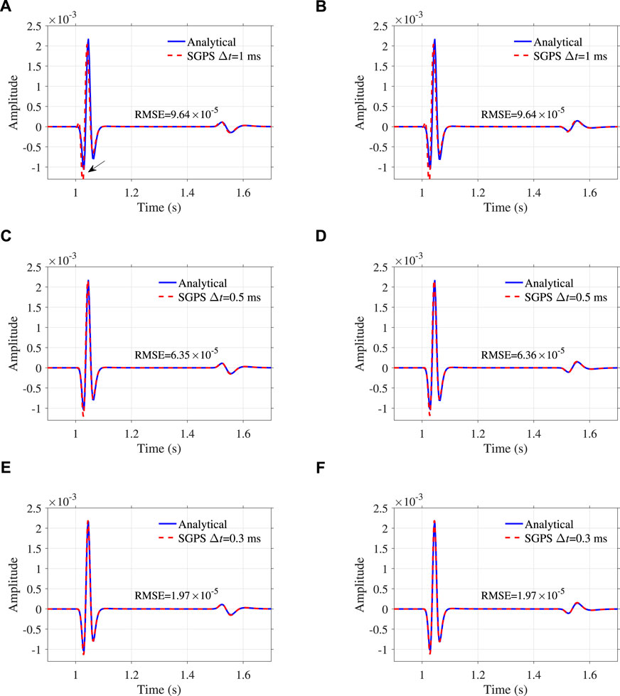
FIGURE 2. Comparison of traditional SGPS numerical solutions with analytical solutions where (A,C,E) depict v_x, (B,D,F) show v_z. The arrows mark visible amplitude differences caused by time dispersion.

Regarding the computational time for a maximum simulation time of 5.4 s, the low-rank extrapolation with Δt = 2.3 ms and the traditional SGPS extrapolation with Δt = 0.3 ms take 322.55 s and 915.68 s, respectively, which means an approximate efficiency gain of 2.8 achieved by the low-rank scheme. All the codes are programming using the MATLAB language and run with a hardware of Intel(R) Xeon(R) Silver-4210 CPU @2.20GHz/2.19 GHz.

A two-layer model with sharp velocity contrasts

Next, we use a two-layer model with sharp velocity contrasts to observe the stability and accuracy of the low-rank temporal extrapolation. The model has 820 × 820 grid points with the grid interval of 10 m. A horizontal interface at z = 4100 m splits the model into two parts: c_p = 2 km/s, c_s = 1.6 km/s, ρ = 1.5 g/cm³, Q_p = 30, Q_s = 15 for the upper layer and c_p = 4 km/s, c_s = 2.5 km/s, ρ = 2.0 g/cm³, Q_p = 60, Q_s = 30 for the lower layer. A Ricker wavelet with the dominant frequency of 30 Hz is located at (x, z) = (4100, 3600) m and is imposed to v_z. The reference frequency is set to w_o = 188.50 rad/s and the ranks of m = n = 2 are used. A timestepping size of Δt = 2.5 ms is used for the low-rank temporal extrapolation, which corresponds to c_pΔt/h = 1.0, far beyond the CFL stability condition of SGPS.

Although such a large timestepping size is used, the low-rank temporal extrapolation is still stable, as shown by the wavefield snapshots at t = 1 s in Figures 3A,B. We also display the computed snapshots by the traditional SGPS scheme with a smaller timestepping size Δt = 1 ms in Figures 3C,D, where visible waveform distortion caused by time dispersion can be observed. When Δt further reduces to 0.5 ms, the time dispersion becomes weaker, as shown in Figures 3E,F. The pointwise FFT scheme is used in the traditional SGPS simulations to account for the spatially variable fractional orders, which means the fractional Laplacians in the top and lower layers are calculated separately. The low-rank decomposition of the P- and S-wave parameters dependent k-space operators takes 74.41 s and the temporal extrapolation for a maximum recording time of 5 s takes 3496.80 s. In comparison, the traditional SGPS extrapolation with Δt = 0.5 ms for the same recording time takes 11,488.52 s, which means the low-rank scheme saves the computational time approximately by 69%. Figure 4 further displays the decoupled P and S wavefields corresponding to the snapshots in Figures 3A,B, which shows a clear separation of P and S waves, despite of some weak noise at the interface.

FIGURE 3

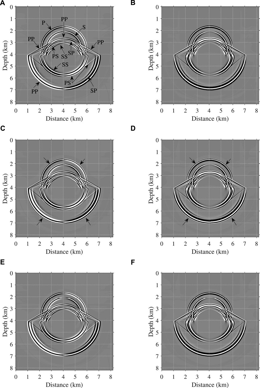
FIGURE 3. Snapshots of v_x: (A,C,E), and v_z: (B,D,F) at t = 1 s by low-rank scheme with Δt = 2.5 ms (A,B), SGPS with Δt = 1 ms (C,D), SGPS with Δt = 0.5 ms (E,F). The symbol ‘PS’ denotes reflection or transmission S waves with incident P waves. The physical meanings of ‘PP’, ‘SS’ and ‘SP’ can be understood in the same way. The arrows in (C,D) indicate the time dispersion.

FIGURE 4

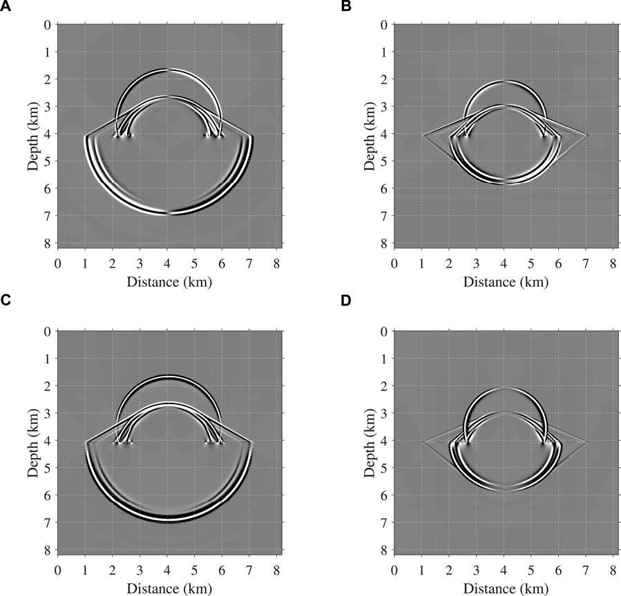
FIGURE 4. Wave mode decoupled snapshots of (A,B) v_x and (C,D) v_z, corresponding to the snapshots in Figures 3A,B. (A,C) show the decoupled P waves and (B,D) show the decoupled S waves.

Wave propagation in complex models

We finally demonstrate the accuracy of the low-rank temporal extrapolation scheme by simulating wave propagation in a modified Marmousi-II model in Figure 5, which is obtained by modifying the shallow part of the original model (Martin et al., 2006) and doing smoothing. The Q model is generated from the velocity model using an empirical formula $Q_l=10{(c_l/1000)}^{2.2},l\in \left\{p,s\right\}$, which results in a minimum Q_p of 24.4 and a minimum Q_s of 15. The grid spacing is 12.5 m. A Ricker wavelet with a dominant frequency of 10 Hz is placed at (x, z) = (3750, 125) m and is applied to v_z as a source. We set Δt = 1.8 ms corresponding to c_pΔt/h = 0.6768, which is beyond of the maximum CFL number required by the traditional SGPS scheme. To demonstrate the low-rank decomposition accuracy in such complex models, we use the ranks of m = n = 6, 5, and 4, respectively. The decomposition using m = n = 6 introduces small errors, with the error magnitudes 10⁶–10⁷ times smaller than the exact operators, as shown in Figures 6B, 7B. As the ranks reduce to 5 and 4, the decomposition errors increase, however they are still much smaller than the exact operators (approximately four orders of magnitude smaller than the latter), as depicted in Figures 6, 7. The subsequent snapshots comparison indicate that the ranks of m = n = 4 can ensure a sufficient accuracy for wave propagation in this model. Regarding the computational cost of the low-rank decomposition, the decompositions with the ranks of 6, 5, and 4 take 218.28 s, 137.77 s and 79.85 s, respectively.

FIGURE 5

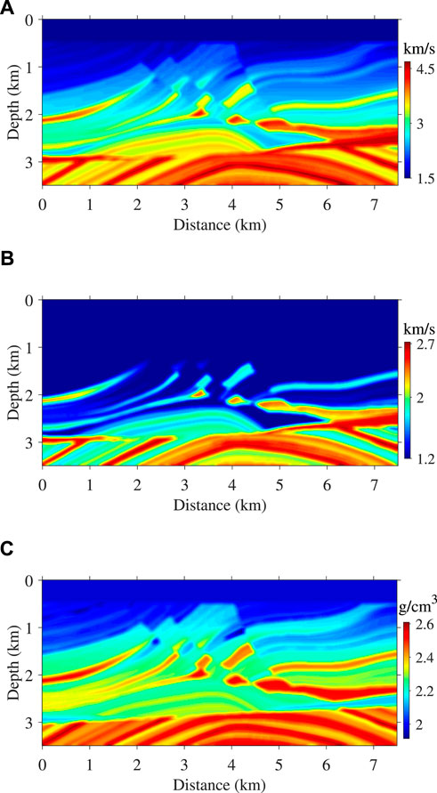
FIGURE 5. A modified Marmousi-II model consisting of 600 × 280 grid points with the grid spacing of 12.5 m: (A) P-, (B) S-wave velocities, and (C) density. The Q model is generated from velocity using an empirical formula $Q_l=10{(c_l/1000)}^{2.2},l\in \left\{p,s\right\}$.

FIGURE 6

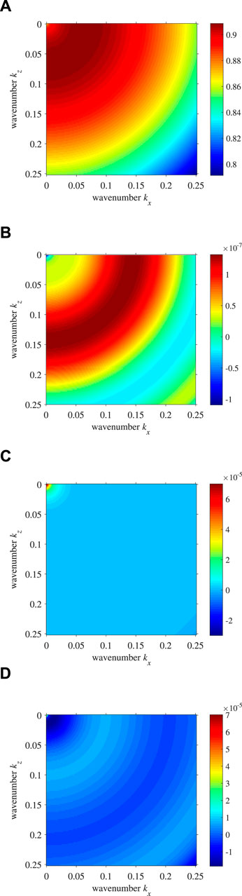
FIGURE 6. Demonstration of low-rank decomposition accuracy: (A) exact ξ_p at (x, z) = (4125, 1125) m where c_p = 2073 m/s and Q_p = 50, low-rank decomposition errors with ranks of (B) m = n = 6, (C) m = n = 5, and (D) m = n = 4.

FIGURE 7

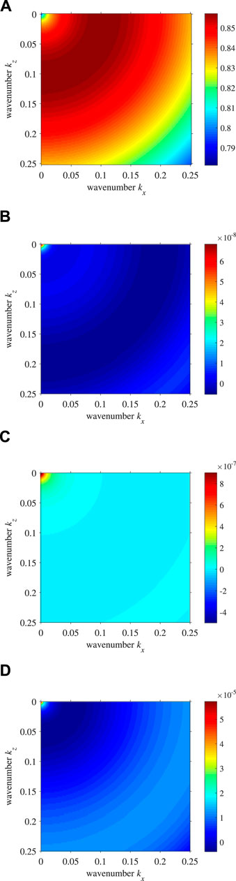
FIGURE 7. Demonstration of low-rank decomposition accuracy: (A) exact ξ_s at (x, z) = (1250, 2925) m where c_s = 1627 m/s and Q_s = 29, low-rank decomposition errors with ranks of (B) m = n = 6, (C) m = n = 5, and (D) m = n = 4.

Considering the low-rank decomposition with m = n = 6 is highly accurate, the simulated wavefield snapshots by this method are used as references (Figures 8C,D) to evaluate the simulated results using smaller ranks. Figures 8E,F indicate that the differences from the references caused by m = n = 4 are approximately 10⁴ times smaller in magnitude than the references. When the ranks decrease to m = n = 3, the differences become larger, however still 100 times smaller in magnitude than the references, as displayed in Figures 8G,H. For a complete comparison, Figures 8A,B display the elastic wavefield snapshots at the same time, showing stronger amplitudes due to the absence of Q effects. Figure 9 further compares the seismic traces recorded at (x, z) = (2375, 12.5) m and (x, z) = (6125, 12.5) m, showing a good match between the calculated traces with the ranks m = n = 4 and the references. The results imply that setting m = n = 4 is sufficient to ensure the wavefield temporal extrapolation accuracy in the Marmousi model.

FIGURE 8

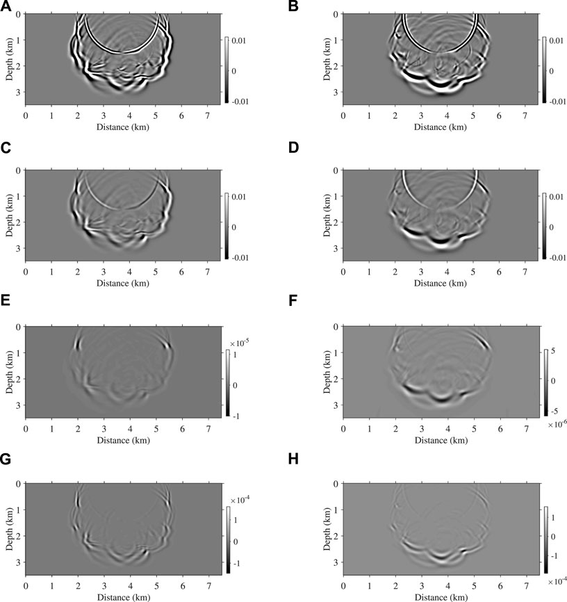
FIGURE 8. Simulated snapshots for v_x (A,C), for v_z (B,D) at t = 1.26 s (A,B) show the snapshots in ealstic media, (C,D) are the viscoelastic snapshots computed by the low-rank scheme with the ranks of m = n = 6. (E,F) show the differences between the results with m = n = 4 and those with m = n = 6. (G,H) show the differences between m = n = 3 and m = n = 6.

FIGURE 9

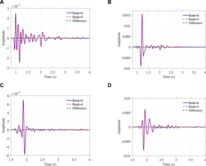
FIGURE 9. Observed seismic traces at (x, z) =(2375, 12.5) m (A,B), at (6125, 12.5) m (C,D). Panels (A,C) for v_x and (B,D) for v_z.

Discussion

The above numerical examples verify the accuracy of the viscoelastic low-rank temporal extrapolation scheme. This scheme can be used as a highly accurate forward modeling tool in viscoelastic media. However, when applying the low-rank temporal extrapolation for Q-RTM, one needs to modify Eq. 21c, Eq. 21d, Eq. 21e, Eq.21f slightly by reversing the plus signs in front of τ_p and τ_s to minus and reversing the minus in front of τ_l in Eq. 24 to a plus. This is actually equavilent to changing the exponential decay term in the analytical solution in Eq. 12 to an exponential growth term. This realizes amplitude compensation only, while preserving the phase unchanged, which is a key point in Q-RTM (Zhu et al., 2014).

Another aspect deserving to address is the choice of the ranks in the low-rank decomposition. Generally, it is difficult to give a strict formula to guide the choice of the ranks, because low-rank decomposition accuracy depends on the timestepping size Δt, velocity and Q spatial structures. As Δt and the model complexity increase, one should increase the ranks to ensure the wave propagation accuracy. According to the Marmousi example and more conducted tests but not shown here, we observe that a desirable choice of ranks should guarantee the relative error of the low-rank decomposition approximately smaller than 1 × 10^–4. This implies that an iterative process can be used to determine the ranks. After setting a threshold and initial ranks, one can do the low-rank decomposition repeatedly and increase the ranks gradually, until the low-rank decomposition error becomes smaller than the threshold. At each time of low-rank decomposition, one only needs to calculate the decomposition errors at several representative positions, such as the positions where the maximum or minimum velocities appear. Considering the low-rank decomposition is conducted before wavefield temporal extrapolation, the computational cost for determining the ranks is negligible.

Note that in the first homogeneous model example, we set ranks of m = n = 1 in the low-rank modeling scheme. In fact, the low-rank calculations in Eq. 27 is not required for homogeneous media, because the wavenumber response does not depend on the space and it can be implemented directly in the Fourier domain. Even so, the low-rank temporal extrapolation with m = n = 1 still works correctly, which means the low-rank decomposition algorithm lets W₁ ≡I and G_1,1 ≡ 1 automatically in Eq. 26.

Finally, we discuss the possibility to set different ranks in low-rank decomposition of the P- and S-wave dependent PSDO. Considering the S-wave velocity is smaller than the P-wave velocity, we try to use smaller ranks in low-rank approximation of the S-wave dependent k-space operator. To form a comparison with the results in Figure 6D, we show the exact ξ_s and the low-rank approximation errors at the same position. Comparison of Figures 10A, 6D indicates the same magnitude order of exact ξ_s and ξ_p. However, when the same ranks of 4 are applied, the low-rank decomposition of ξ_s introduces a smaller error than that of ξ_p, as shown in Figure 10B. When the ranks of ξ_s decrease to 3, the error magnitude is similar to that of the low-rank decomposition of ξ_p with the ranks of 4, as shown in Figure 10C. These results indicate that when approximating the wave mode dependent k-space operators, smaller ranks can be used in the low-rank decomposition of S-wave dependent operators, which helps to reduce the overall computational cost.

FIGURE 10

FIGURE 10. Demonstration of low-rank decomposition accuracy: (A) exact ξ_s at (x, z) = (4125, 1125) m where c_s = 1200 m/s and Q_s = 15, low-rank decomposition errors with ranks of (B) m = n = 4, and (C) m = n = 3. These results form comparisons with Figure 6D.

Conclusion

We have developed a highly accurate temporal extrapolation scheme for a novel fractional Laplacians constant-Q viscoelastic wave equation that can be used to describe seismic attenuation in the earth. The temporal extrapolation formula is derived from the general solution of the viscoelastic wave equation system, which makes the extrapolation free of numerical dispersion and instability in homogeneous media. A low-rank approximation of the k-space operators is further applied to implement the temporal extrapolation efficiently in heterogeneous media. The computational cost of the low-rank scheme at each extrapolation step is proportional to the ranks involved in the low-rank decomposition. Numerical results with the Marmousi model indicate that application of the ranks of m = n = 4 can provide sufficient accuracy in the case of a CFL number of 0.67 (beyond the value required by the traditional stability condition). Another two benefits of the low-rank temporal extrapolation is automatical treatment to the spatial variable-order fractional Laplacians and separation of compressional and shear waves. In general, the developed low-rank temporal extrapolation scheme can be used as a highly accurate seismic modeling tool in attenuating media and can also act as a forward engine in attenuation compensated reverse-time migration algorithms.

Data availability statement

The raw data supporting the conclusions of this article will be made available by the authors, without undue reservation.

Author contributions

HC contributes to the mathematical derivations, the low-rank decomposition algorithm and writes the main body of this paper. LZ writes the viscoelastic forward modeling codes and HZ contributes to numerical examples and figures.

Funding

This research is supported by National Key Research and Development Program of China (Grant No. 2018YFA0702502), the National Natural Science Foundation of China (Grant No. 42274143, U19B6003-04, 41804111), and R&D Department of China National Petroleum Corporation (Investigations on fundamental experiments and advanced theoretical methods in geophysical prospecting applications, Grant No. 2022DQ0604 -01/03).

Conflict of interest

The authors declare that the research was conducted in the absence of any commercial or financial relationships that could be construed as a potential conflict of interest.

Publisher’s note

All claims expressed in this article are solely those of the authors and do not necessarily represent those of their affiliated organizations, or those of the publisher, the editors and the reviewers. Any product that may be evaluated in this article, or claim that may be made by its manufacturer, is not guaranteed or endorsed by the publisher.

References

Blanch, J. O., Robertsson, J. O., and Symes, W. W. (1995). Modeling of a constant Q: Methodology and algorithm for an efficient and optimally inexpensive viscoelastic technique. Geophysics 60, 176–184. doi:10.1190/1.1443744

CrossRef Full Text | Google Scholar

Caputo, M. (1967). Linear models of dissipation whose Q is almost frequency independent—Ii. Geophys. J. Int. 13, 529–539. doi:10.1111/j.1365-246x.1967.tb02303.x

CrossRef Full Text | Google Scholar

Carcione, J., Cavallini, F., Mainardi, F., and Hanyga, A. (2002). Time-domain modeling of constant- Q seismic waves using fractional derivatives. Pure Appl. Geophys. 159, 1719–1736. doi:10.1007/s00024-002-8705-z

CrossRef Full Text | Google Scholar

Carcione, J. M. (2010). A generalization of the Fourier pseudospectral method. Geophysics 75, A53–A56. doi:10.1190/1.3509472

CrossRef Full Text | Google Scholar

Carcione, J. M., Kosloff, D., and Kosloff, R. (1988). Wave propagation simulation in a linear viscoelastic medium. Geophys. J. Int. 95, 597–611. doi:10.1111/j.1365-246x.1988.tb06706.x

CrossRef Full Text | Google Scholar

Chen, H., Zhou, H., Li, Q., and Wang, Y. (2016). Two efficient modeling schemes for fractional Laplacian viscoacoustic wave equation. Geophysics 81, T233–T249. doi:10.1190/geo2015-0660.1

CrossRef Full Text | Google Scholar

Chen, H., Zhou, H., and Rao, Y. (2020a). An implicit stabilization strategy for Q-compensated reverse time migration. Geophysics 85, S169–S183. doi:10.1190/geo2019-0235.1

CrossRef Full Text | Google Scholar

Chen, H., Zhou, H., and Rao, Y. (2021). Constant-Q wave propagation and compensation by pseudo-spectral time-domain methods. Comput. Geosciences 155, 104861. doi:10.1016/j.cageo.2021.104861

CrossRef Full Text | Google Scholar

Chen, H., Zhou, H., and Rao, Y. (2020b). Source wavefield reconstruction in fractional laplacian viscoacoustic wave equation-based full waveform inversion. IEEE Trans. Geosci. Remote Sens. 59, 6496–6509. doi:10.1109/tgrs.2020.3029630

CrossRef Full Text | Google Scholar

Chen, H., Zhou, H., and Zu, S. (2017). “Simultaneous inversion of velocity and q using a fractional laplacian constant-q wave equation,” in Proceedings of the 79th EAGE Conference and Exhibition 2017, Paris, France, June 12-15, 2017 (Palermo, Italy: European Association of Geoscientists & Engineers), 1–5.2017

CrossRef Full Text | Google Scholar

Chu, C., and Stoffa, P. L. (2010). “Acoustic anisotropic wave modeling using normalized pseudo-Laplacian,” in SEG technical Program expanded abstracts 2010 (Texas, United States: Society of Exploration Geophysicists), 2972–2976.

Google Scholar

Etgen, J. T., and Dellinger, J. (1989). Accurate wave-equation modeling. Seg. Annu. Meet. (OnePetro) 1989, 494–497. doi:10.1190/1.1889673

CrossRef Full Text | Google Scholar

Fang, G., Fomel, S., Du, Q., and Hu, J. (2014). Lowrank seismic-wave extrapolation on a staggered grid. Geophysics 79, T157–T168. doi:10.1190/geo2013-0290.1

CrossRef Full Text | Google Scholar

Fomel, S., Ying, L., and Song, X. (2013). Seismic wave extrapolation using lowrank symbol approximation. Geophys. Prospect. 61, 526–536. doi:10.1111/j.1365-2478.2012.01064.x

CrossRef Full Text | Google Scholar

Huang, J., and Liu, H. (2020). New k-space scheme for modeling elastic wave propagation in heterogeneous media. Chin. J. Geophys. 63, 3091–3104. doi:10.6038/cjg2020N0291

CrossRef Full Text | Google Scholar

Kjartansson, E. (1979). Constant Q-wave propagation and attenuation. J. Geophys. Res. 84, 4737–4748. doi:10.1029/jb084ib09p04737

CrossRef Full Text | Google Scholar

Koene, E. F., Robertsson, J. O., Broggini, F., and Andersson, F. (2018). Eliminating time dispersion from seismic wave modeling. Geophys. J. Int. 213, 169–180. doi:10.1093/gji/ggx563

CrossRef Full Text | Google Scholar

Li, Q., Zhou, H., Zhang, Q., Chen, H., and Sheng, S. (2016). Efficient reverse time migration based on fractional Laplacian viscoacoustic wave equation. Geophys. J. Int. 204, 488–504. doi:10.1093/gji/ggv456

CrossRef Full Text | Google Scholar

Martin, G. S., Wiley, R., and Marfurt, K. J. (2006). Marmousi2: An elastic upgrade for marmousi. Lead. edge 25, 156–166. doi:10.1190/1.2172306

CrossRef Full Text | Google Scholar

Mu, X., Huang, J., Wen, L., and Zhuang, S. (2021). Modeling viscoacoustic wave propagation using a new spatial variable-order fractional Laplacian wave equation. Geophysics 86, T487–T507. doi:10.1190/geo2020-0610.1

CrossRef Full Text | Google Scholar

Mu, X., Huang, J., Yang, J., Li, Z., and Ssewannyaga Ivan, M. (2022). Viscoelastic wave propagation simulation using new spatial variable-order fractional Laplacians. Bull. Seismol. Soc. Am. 112, 48–77. doi:10.1785/0120210099

CrossRef Full Text | Google Scholar

Pestana, R. C., and Stoffa, P. L. (2010). Time evolution of the wave equation using rapid expansion method. Geophysics 75, T121–T131. doi:10.1190/1.3449091

CrossRef Full Text | Google Scholar

Sun, J., Fomel, S., Sripanich, Y., and Fowler, P. (2017). Recursive integral time extrapolation of elastic waves using low-rank symbol approximation. Geophys. J. Int. 211, 1478–1493. doi:10.1093/gji/ggx386

CrossRef Full Text | Google Scholar

Sun, J., Zhu, T., and Fomel, S. (2015). Viscoacoustic modeling and imaging using low-rank approximation. Geophysics 80, A103–A108. doi:10.1190/geo2015-0083.1

CrossRef Full Text | Google Scholar

Wang, N., Xing, G., Zhu, T., Zhou, H., and Shi, Y. (2022). Propagating seismic waves in vti attenuating media using fractional viscoelastic wave equation. JGR. Solid Earth 127, e2021JB023280. doi:10.1029/2021jb023280

CrossRef Full Text | Google Scholar

Wang, N., Zhou, H., Chen, H., Xia, M., Wang, S., Fang, J., et al. (2018). A constant fractional-order viscoelastic wave equation and its numerical simulation scheme. Geophysics 83, T39–T48. doi:10.1190/geo2016-0609.1

CrossRef Full Text | Google Scholar

Wang, Y., Zhou, H., Chen, H., and Chen, Y. (2018). Adaptive stabilization for Q-compensated reverse time migration. Geophysics 83, S15–S32. doi:10.1190/geo2017-0244.1

CrossRef Full Text | Google Scholar

Xing, G., and Zhu, T. (2022). Decoupled fréchet kernels based on a fractional viscoacoustic wave equation. Geophysics 87, T61–T70. doi:10.1190/geo2021-0248.1

CrossRef Full Text | Google Scholar

Xing, G., and Zhu, T. (2020). “Hessian-based multiparameter fractional viscoacoustic full-waveform inversion,” in Proceedings of the SEG International Exposition and Annual Meeting (OnePetro), October 11–16, 2020.

CrossRef Full Text | Google Scholar

Xing, G., and Zhu, T. (2019). Modeling frequency-independent Q viscoacoustic wave propagation in heterogeneous media. J. Geophys. Res. Solid Earth 124, 11568–11584. doi:10.1029/2019jb017985

CrossRef Full Text | Google Scholar

Xue, Z., Baek, H., Zhang, H., Zhao, Y., Zhu, T., and Fomel, S. (2018). “Solving fractional Laplacian viscoelastic wave equations using domain decomposition,”, Proceedings of the SEG International Exposition and Annual Meeting (OnePetro), California, USA, August 2018, 3943–3947.2018

CrossRef Full Text | Google Scholar

Yan, J., and Liu, H. (2016). Modeling of pure acoustic wave in tilted transversely isotropic media using optimized pseudo-differential operators. Geophysics 81, T91–T106. doi:10.1190/geo2015-0111.1

CrossRef Full Text | Google Scholar

Yang, J., and Zhu, H. (2018). A time-domain complex-valued wave equation for modelling visco-acoustic wave propagation. Geophys. J. Int. 215, 1064–1079. doi:10.1093/gji/ggy323

CrossRef Full Text | Google Scholar

Yang, J., Zhu, H., Li, X., Ren, L., and Zhang, S. (2020). Estimating p wave velocity and attenuation structures using full waveform inversion based on a time domain complex-valued viscoacoustic wave equation: The method. J. Geophys. Res. Solid Earth 125, e2019JB019129. doi:10.1029/2019jb019129

CrossRef Full Text | Google Scholar

Zhang, Y., and Zhang, G. (2009). One-step extrapolation method for reverse time migration. Geophysics 74, A29–A33. doi:10.1190/1.3123476

CrossRef Full Text | Google Scholar

Zhao, X., Zhou, H., Chen, H., and Wang, Y. (2020). Domain decomposition for large-scale viscoacoustic wave simulation using localized pseudo-spectral method. IEEE Trans. Geosci. Remote Sens. 59, 2666–2679. doi:10.1109/tgrs.2020.3006614

CrossRef Full Text | Google Scholar

Zhu, T., and Carcione, J. M. (2014). Theory and modelling of constant-Q p-and s-waves using fractional spatial derivatives. Geophys. J. Int. 196, 1787–1795. doi:10.1093/gji/ggt483

CrossRef Full Text | Google Scholar

Zhu, T., Harris, J. M., and Biondi, B. (2014). Q-compensated reverse-time migration. Geophysics 79, S77–S87. doi:10.1190/geo2013-0344.1

CrossRef Full Text | Google Scholar

Zhu, T., and Harris, J. M. (2014). Modeling acoustic wave propagation in heterogeneous attenuating media using decoupled fractional Laplacians. Geophysics 79, T105–T116. doi:10.1190/geo2013-0245.1

CrossRef Full Text | Google Scholar

Appendix: First-order time-marching equation system

Inserting Eqs. 9, 20 into Eq. 17 gives

$\begin{array}{ll}\hfill \frac{{\tilde{u}}^{n+1}-2{\tilde{u}}^n+{\tilde{u}}^{n-1}}{\mathrm{\Delta }{t}^2}& =-2\left(i{k}_x\right)\left[c_s^{2+2{\gamma }_s}\left(i{k}_z{\xi }_s\right){\tilde{w}}^n+\frac{{\tau }_s{k}^{2{\gamma }_s-1}}{\mathrm{\Delta }t}\left(i{k}_z\right)\left({\tilde{w}}^n-{\tilde{w}}^{n-1}\right)\right]\hfill \\ \hfill & \times \left(i{k}_x\right)\left\{c_p^{2+2{\gamma }_p}\left[\left(i{k}_x{\xi }_p\right){\tilde{u}}^n+\left(i{k}_z{\xi }_p\right){\tilde{w}}^n\right]+\frac{{\tau }_p{k}^{2{\gamma }_p-1}}{\mathrm{\Delta }t}\left[\left(i{k}_x\right)\left({\tilde{u}}^n-{\tilde{u}}^{n-1}\right)+\left(i{k}_z\right)\left({\tilde{w}}^n-{\tilde{w}}^{n-1}\right)\right]\right\}\hfill \\ \hfill & +\left(i{k}_z\right)\left\{c_s^{2+2{\gamma }_s}\left[\left(i{k}_x{\xi }_s\right){\tilde{w}}^n+\left(i{k}_z{\xi }_s\right){\tilde{u}}^n\right]+\frac{{\tau }_s{k}^{2{\gamma }_s-1}}{\mathrm{\Delta }t}\left[\left(i{k}_x\right)\left({\tilde{w}}^n-{\tilde{w}}^{n-1}\right)+\left(i{k}_z\right)\left({\tilde{u}}^n-{\tilde{u}}^{n-1}\right)\right]\right\},\hfill \end{array}$(A-1)

$\begin{array}{ll}\hfill \frac{{\tilde{w}}^{n+1}-2{\tilde{w}}^n+{\tilde{w}}^{n-1}}{\mathrm{\Delta }{t}^2}& =-2\left(i{k}_z\right)\left[c_s^{2+2{\gamma }_s}\left(i{k}_x{\xi }_s\right){\tilde{u}}^n+\frac{{\tau }_s{k}^{2{\gamma }_s-1}}{\mathrm{\Delta }t}\left(i{k}_x\right)\left({\tilde{u}}^n-{\tilde{u}}^{n-1}\right)\right]\hfill \\ \hfill & +\left(i{k}_x\right)\left\{c_s^{2+2{\gamma }_s}\left[\left(i{k}_x{\xi }_s\right){\tilde{w}}^n+\left(i{k}_z{\xi }_s\right){\tilde{u}}^n\right]+\frac{{\tau }_s{k}^{2{\gamma }_s-1}}{\mathrm{\Delta }t}\left[\left(i{k}_x\right)\left({\tilde{w}}^n-{\tilde{w}}^{n-1}\right)+\left(i{k}_z\right)\left({\tilde{u}}^n-{\tilde{u}}^{n-1}\right)\right]\right\}\hfill \\ \hfill & +\left(i{k}_z\right)\left\{c_p^{2+2{\gamma }_p}\left[\left(i{k}_x{\xi }_p\right){\tilde{u}}^n+\left(i{k}_z{\xi }_p\right){\tilde{w}}^n\right]+\frac{{\tau }_p{k}^{2{\gamma }_p-1}}{\mathrm{\Delta }t}\left[\left(i{k}_x\right)\left({\tilde{u}}^n-{\tilde{u}}^{n-1}\right)+\left(i{k}_z\right)\left({\tilde{w}}^n-{\tilde{w}}^{n-1}\right)\right]\right\},\hfill \end{array}$(A-2)

where ξ_p and ξ_s are defined in Eq. 24.

We further introduce the following intermediate variables:

${\tilde{v}}_x^{n+\frac{1}{2}}=\frac{{\tilde{u}}^{n+1}-{\tilde{u}}^n}{\mathrm{\Delta }t},{\tilde{v}}_z^{n+\frac{1}{2}}=\frac{{\tilde{w}}^{n+1}-{\tilde{w}}^n}{\mathrm{\Delta }t},$(A-3)

${\tilde{\sigma }}_{xx}^n=-2\left[c_s^{2+2{\gamma }_s}\left(i{k}_z{\xi }_s\right){\tilde{w}}^n+\frac{{\tau }_s{k}^{2{\gamma }_s-1}}{\mathrm{\Delta }t}\left(i{k}_z\right)\left({\tilde{w}}^n-{\tilde{w}}^{n-1}\right)\right],$(A-4)

${\tilde{\sigma }}_{zz}^n=-2\left[c_s^{2+2{\gamma }_s}\left(i{k}_x{\xi }_s\right){\tilde{u}}^n+\frac{{\tau }_s{k}^{2{\gamma }_s-1}}{\mathrm{\Delta }t}\left(i{k}_x\right)\left({\tilde{u}}^n-{\tilde{u}}^{n-1}\right)\right]$(A-5)

${\tilde{\sigma }}_{xz}^n=c_s^{2+2{\gamma }_s}\left[\left(i{k}_x{\xi }_s\right){\tilde{w}}^n+\left(i{k}_z{\xi }_s\right){\tilde{u}}^n\right]+\frac{{\tau }_s{k}^{2{\gamma }_s-1}}{\mathrm{\Delta }t}\left[\left(i{k}_x\right)\left({\tilde{w}}^n-{\tilde{w}}^{n-1}\right)+\left(i{k}_z\right)\left({\tilde{u}}^n-{\tilde{u}}^{n-1}\right)\right],$(A-6)

${\tilde{P}}^n=c_p^{2+2{\gamma }_p}\left[\left(i{k}_x{\xi }_p\right){\tilde{u}}^n+\left(i{k}_z{\xi }_p\right){\tilde{w}}^n\right]+\frac{{\tau }_p{k}^{2{\gamma }_p-1}}{\mathrm{\Delta }t}\left[\left(i{k}_x\right)\left({\tilde{u}}^n-{\tilde{u}}^{n-1}\right)+\left(i{k}_z\right)\left({\tilde{w}}^n-{\tilde{w}}^{n-1}\right)\right].$(A-7)

Using these new wavefield variables, one can readily rewrite Eq. A-1and Eq. A-2 as the first-order time-marching system in Eq. 21a, Eq. 21b, Eq. 21c, Eq. 21d, Eq. 21e, Eq. 21f.