Microseismic positioning of an isolated working face under complex geological conditions and its engineering application

In view of the inability to accurately locate vibrations in isolated workings under complex geological conditions, an adaptive rotational categorization method, a downhill comparison method based on time-frequency analysis (TFA-DC method), a variable-step acceleration search method, and a dual-phase seismic source location method (TD-DL method) are proposed. A set of integrated software with features of “visualization”, “interactive” and “one-click” was developed for microseismic data processing. Results show that compared with the improved STA/LTA method, the recognition accuracy of the island working face microseismic signal by the adaptive wheel classification method is increased by 4.8%. Compared with the improved STA/LTA method, the TFA-DC method has the advantage that it can simultaneously pick up the exact p wave and the peak S wave, and the failure ratio is 0. Compared with simulated annealing algorithm and genetic algorithm, stepwise accelerated search method has better results. The standard deviation of objective function value, location error and wave velocity error are all 0. Method improves the positioning of the TD - DL detector coordinates, dual phase and coherence of known information, such as the positioning result positioning error is only the p wave and S wave ChanZhen phase positioning method of 9.5% and 14.5%, to a certain extent offset the p wave and S wave ChanZhen phase calculation of the positioning error, so as to improve the effect of source localization precision of the inversion.

1 Introduction

With increase in mining depth and scale, the uncertainty of the underground environment in which it takes place gradually increases, which is manifested by the fact that the primary geological structure of the strata in which it is located is susceptible to extensive disturbance or even destruction. This may imply that the mining of mineral resources may also be accompanied by a number of environmental and safety hazards such as impact pressure, collapse of the mining area, rock explosion, and roofing of the tunnel flake (Pan et al., 2007; Cui et al., 2019; Li et al., 2019).

In order to monitor and prevent these safety hazards, microseismic monitoring technology is now commonly used in the mining process to monitor and locate disaster sources (Gong et al., 2010; Gong et al., 2012). This predicting is necessary as part of monitoring the rock interface damage, matrix or inclusions fracture during the mining process to ensure the safety of construction and reduce economic losses (Li and Xu, 2020). The core elements of microseismic monitoring are phase identification, arrival time pickup, algorithm optimization, and source localization.

For seismic phase recognition, Zhao et al. (2015) used microseismic waveform repetition, tail-wave drop, signal principal frequency, and occurrence time that fall under Fisher classification method parameters to construct a seismic phase recognition model. Dong et al. (2016) selected microseismic occurrence time, seismic moment, total radiated energy, P- and S-wave energy ratio, corner frequency, and static stress drop as feature parameters for microseismic recognition. Used Fisher classification method, and Plain Bayes method and logistic regression were used for classification. Jiang et al. (2021) proposed an earthquake phase identification method based on random forest classifier after reducing the data volume by singular value decomposition and used the time-frequency characteristics of microseismic signals. Wu et al. (2016) proposed an earthquake phase identification method based on S-transform, and the similarity of phase and frequency and random combination analysis of P-wave waveform.

In arrival pickup, Ross et al. (2018) proposed a method for the P-wave arrival pickup and the initial motion polarity determination using deep learning. Perol et al. (2018) proposed a method for seismic phase identification and arrival pickup based on U-shaped neural networks. Lee et al. (2017) proposed a modified energy ratio (MER) method for arrival pickup. Diehl et al. (2009) proposed a method for the P-wave arrival pickup based on a hybrid STA/LTA-Polarization-AIC algorithm. for P-wave arrival pickup is proposed based on the short time-window average/long time-window average (STA/LTA), polarization and AIC criteria.

In terms of optimization of algorithms, Li et al. (2014) proposed a simplex shape localization method based on L1 parametric statistics, which had high immunity to outliers with large deviations. Jia et al. (2017) analyzed the relationship between localization error and the number and location of sensors using high-density table-array and particle swarm algorithms. In the source location, the joint inversion localization method is more common (Li et al., 2013; Zheng et al., 2016; Xue et al., 2018), and there are many other methods, Wang et al. (2019) proposed a differential evolutionary microseismic localization method with improved localization objective function for traditional localization method which relied heavily on the walking time accuracy. Wang et al. (2020) proposed a hybrid microseismic source localization algorithm based on simplex-shortest path ray tracing.

The above research results have improved the accuracy of earthquake source localization to a certain extent, but there are some shortcomings. For the seismic phase identification, the commonly used STA/LTA method calculates the ratio of the long- and short-time windows of the whole signal, and the invalid background noise in the whole signal accounts for most of it, resulting in lot of arithmetic power and time; for the arrival pickup, with the increase of the geophone arrangement density (Jia et al., 2017; Zhao et al., 2019), the quality of the waveforms collected by each geophone is increasingly different for poor quality signals. Therefore, for some of the poor quality signals, even if the high-precision pickup method is used, the pickup results will have large errors, leading to an increase in the source inversion error. For optimization algorithms, traditional algorithms such as genetic algorithms and simulated annealing algorithms usually rely on the selection of iterative initial parameters, which may lead to distorted or scattered localization calculation results if they are not selected properly (Tian and Chen, 2002). Due to their fixed search step, these may also lead to poor accuracy or convergence of localization results. For different objective functions, and initial data (including geophone coordinates, P-wave initial value arrival time, etc.), the localization effect may occur for source localization, and hence it may be difficult to recognize the accurate initial arrival time of the single phase of the S-wave due to interference with other phases. On this basis, the current utilization of the S-wave single-phase relative to source localization is not high. The difference and connection between P-wave single-phase and S-wave single-phase in source localization are not clarified; the effect of source localization using S-wave arrival time alone is unknown.

Aiming at the above existing problems, by means of theoretical analysis, algorithm programming, numerical calculation and engineering verification, the adaptive wheel classification seismic phase identification method and time-frequency analysis-downhill comparison method (TFA-DC Method) are put forward respectively. The phases location method for the double seismic phase is TFA-DC-double Seismic Phases (TD-DL method), and the optimization algorithm of accelerated search with variable step size. And integrated into interactive microseismic signal processing software, the source inversion and location results can be obtained by one-click through the original signal, which provides a new feasible scheme for real-time microseismic monitoring.

2 Project overview

2.1 Geological conditions of the 8204–2 working face of Tashan Mine

Tashan Mine is a model mine in Datong area, and is a mega mine with the largest design capacity, with an annual production of 15 million tons of coal in China. The project team conducted several field surveys of the Tashan Mine and finally selected the 8204–2 working face in the second pan area as the basis for the study. The mine conditions of 8204–2 working face of Tashan Mine are as follows:

Tashan mine 8204–2 working face is an isolated island working face, coal seam mining depth is about 500 m, coal seam thickness is 12–20 m averaging about 15 m, coal seam dip angle is 2–5°, uses comprehensive mining, the working face length is about 150 m, advances 10 cuts per day of about 8 m, and has no underground monitoring system.

Therefore, in view of the geological conditions at Datong Tashan Mine, the microseismic monitoring system was placed at the 8204–2 working face in the second pan area.

2.2 Tower hill mine introduction to microseismic monitoring

The initial selection of the site of the stations was based on the above-ground and below-ground comparison map of the 8204–2 working face of the Tashan Mine, which required each station to cover the 8204–2 working face as much as possible, and there should be no “three points and one line” between each ground station, which is conducive to observation and data processing (Jia et al., 2017). It was planned to set up 11 alternative ground monitoring stations in the mine. Initially, seven stations were set up for observations, and later, if necessary, 1–2 stations were set up according to the results from the observations, and key monitoring areas. After repeated surveys of the pre-selected locations, the specific locations of the seven ground monitoring stations were finally determined. The precise mine coordinates of the ground monitoring stations were measured on site by GPS positioning equipment at the mine site, as shown in Table 1.

TABLE 1

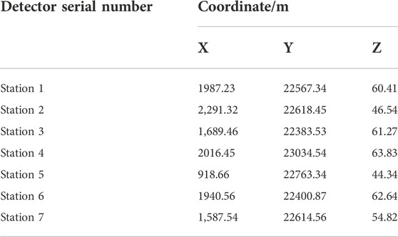
TABLE 1. Coordinates of mining area of station.

As shown in Table 1, the distribution map of the ground monitoring stations in the mining area with seven stations is drawn, as shown in Figure 1, where the red mark is the location of the selected ground monitoring stations.

FIGURE 1

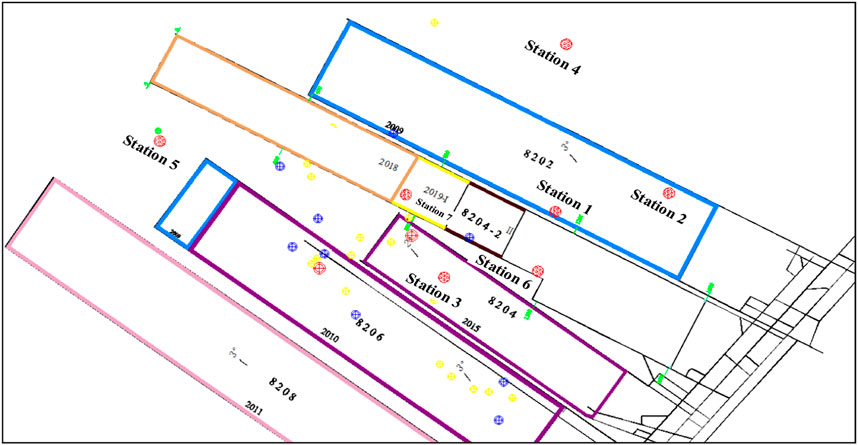
FIGURE 1. Distribution of ground monitoring stations in mining area.

2.2.1 High-frequency microseismic collector architecture

The high-frequency microseismic signal collector consisted of a data collector, a three-component vibration velocity sensor, a GPS timing system, and a Wi-Fi transmission module.

The data collector consists of a first- and second preamplifier, an analog-to-digital conversion unit, a data storage unit, a control unit, a display, a hard disk, a USB module, a Wi-Fi interface, and a power supply module. The data collector adopted high-frequency data acquisition and synchronous segment index compression technology to achieve high-speed retrieval, high-precision data segmentation and rapid upload, and high efficiency in post-processing to browse data, count overall parameters, and sieve valid data.

Three-component high-frequency vibration velocity sensor was used to have complete, continuous signal acquisition, three-component vibration velocity sensors were assembled from one vertical and two horizontal sensors, which monitored the vibration signal in three directions: east-west, north-south, and vertical velocity, Each sensor was such that it covered a circular area of 1–2 km of monitoring, with the frequency of vibration velocity signal within 10–1,400 kHz flat response, high signal-to-noise ratio, small phase difference, high dynamic resolution, and strong temperature adaptability.

The collector equipment was IP68 rated for water and dust resistance and is equipped with 4 TB of space for binary stream data storage. Each collector is designed with eight sampling channels, which had a sampling channel sampling frequency of up to 10 kHz with a sensitivity of 100 ± 5% (V/m/s). A three-component vibration velocity sensor has six channels, GPS timing system occupies one channel, and the remaining one channel can be connected to other sensors. The design of the high-frequency micro-vibration collector is shown in Figure 2.

FIGURE 2

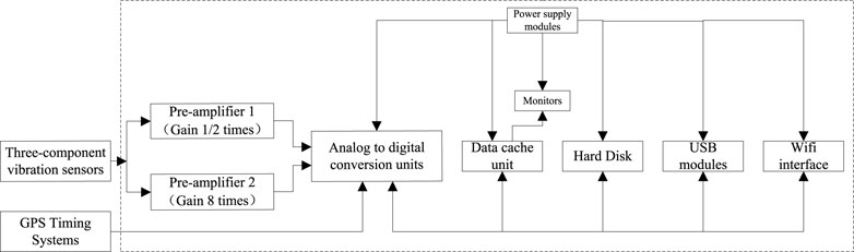
FIGURE 2. Structure of the high frequency microseismic collector.

The GPS timing system determines the ground station data sampling time with the Earth coordinates of the ground station, occupying one acquisition channel of the data collector. The data collector uses its external port to read the PPS (Pulse Per Second) signal of the GPS timing system to synchronize with the vibration signal with a timing accuracy of 10 µs,, to ensure the sampling accuracy of 10 kHz of the data collector.

The Wi-Fi transmission module has the wireless transmission support of the data collector and the speed-sensor sensing data, which are, in turn, connected to the bridge data transmitter.

3 Details on the microseismic phase identification and the seismic source localization methods

3.1 Adaptive rotation categorization method fundamentals

The adaptive rotational categorization method consists of four main steps which are as follows::

1) Adaptive high-pass filtering

In order to reduce the interference of the background noise on the microseismic response and to improve the recognition accuracy and algorithm stability of the adaptive rotational categorization method, high-pass filtering of the original signal was required, and the lower high-pass filtering limit required for high-pass filtering needed to be entered manually. Therefore, in order to realize automatic process operation of the whole method, an adaptive high-pass filtering processing method that can process various forms of microseismic signals is needed.

For the automated operation of high-pass filtering, here a base over-zero rate was used, which used the period function to discriminate the period (the number of times it crosses the X-axis from bottom up per unit time) to estimate the frequency of the main trend waveform with higher energy and stable frequency in the intercepted signal. The number of times the signal crosses the X-axis from bottom up in 10 s is 9, so the base rate was 0.9 Hz. The number of segments of the intercepted signal calculated is shown in Figure 3.

2) Calculation of the upper and lower bounds of the background noise amplitude

FIGURE 3

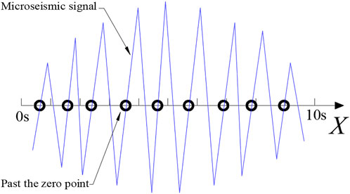
FIGURE 3. Calculation diagram of basic zero-crossing rate.

In order to further bring out the microseismic response signal, and determine the basis for taking the radius of rotation circle R_w (mm/s) after the original signal had undergone the adaptive high-pass filtering to improve the signal-to-noise ratio, the 95% probability of the falling point in the horizontal axis interval (μ-2σ,μ+2σ) of the normal distribution was introduced as the confidence interval of the signal. This, method gradually used increasing the coverage from Y=0, and judging whether the whole signal was included. The method of 95% of data points was used to iteratively compare the upper and lower bounds of the background noise amplitude that satisfied the above conditions to ensure that the obtained results covered most of the background noise, invalid responses, and filtered out the microseismic response signals.

3) Rotation circle radius calculation and rotation iteration

A small number of higher amplitude data points were selected from a single microseismic response that provided the base data for the next step of grouping the exceedance points into categories. The center of the rotating circle was located on the X-axis, and its radius was taken as the range expansion factor, Q, times the distance between the upper bound D_u (mm/s) and the lower bound D_d (mm/s) of the background noise amplitude. By traversing all data points of the whole signal and comparing them, the data points larger than the radius R_w of the rotating circle were filtered out to obtain all the exceedance points needed for the next step. The iterative screening used the average of the absolute values of the two elements before and after in the whole segment signal to represent the amplitude of the signal here. This, increased the applicable range of the iterative comparison, and avoided the identification error caused by the radical change of a single data point.

4) Clustering of exceedance points

In order to finally obtain the influence region of the microseismic response in the microseismic signal, i.e., to identify the seismic phase of the whole microseismic signal, the overruns selected by the rotation circle needed to be grouped into the same group to represent a single seismic phase identification result, and into multiple groups to represent multiple seismic phase identification results. If the time difference between the two was greater than the grouping interval, F_int, the points were grouped into one category, after which the points were grouped into the next category.

3.2 TFA-DC method determine the pickup time

Speech and power density spectrograms were used to obtain the location and regularity of the background noise and the change of frequency, amplitude and energy of the microseismic signal before and after the initial arrival of P-wave and the S-waves. On this basis, the FIR band-pass filtering was carried out twice continuously with the main frequency of the S-wave as the circle point, and the specified filtering range in radius was used to filter out the high and low frequency background noise with regularity and power greater than that of P-wave and S-wave signals. This made the power density spectrogram of the S-wave of the main frequencies clearly appear, and also made the signal image smoother and more suitable for iterative comparison. Based on the above theoretical results, the TFA-DC method for the joint pickup of the P-wave and S-wave dual-oscillation phase arrivals was used by setting the mathematical expression of the full-subwave amplitude as a threshold, and followed three major relationships between the P-wave and the S-wave power magnitude, the arrival sequence, and the waveform overlap.

3.2.1 Connection between P wave and S wave

After analyzing the original signal by speech spectrogram and power density spectrogram and using two consecutive FIR bandpass filtering, the three relations between p wave and S wave are as follows: power magnitude relationship, arrival sequence relationship, waveform overlap relationship.

1) Power relationship

The power and amplitude of S wave in the microseismic signal are larger than that of p wave, so the amplitude surge caused by the initial arrival of the microseismic signal is mainly caused by the arrival of S wave, so the seismic pickup by S wave is more concise than that by p wave.

2) The relationship of arrival sequence

In most cases, p wave velocity is greater than S wave velocity, so p wave should arrive at the detector first than S wave. That is, from the perspective of microseismic signal waveform, the shock change of microseismic signal waveform caused by the arrival of p wave should be on the left side of the shock change of microseismic signal waveform caused by the arrival of S wave.

3) Waveform overlap relationship

Usually, the distance between the seismogenic position and the detector is relatively small, so it is difficult to completely calm the mechanical vibration caused by the initial arrival of p wave before the arrival of S wave. Therefore, the p wave shape should overlap with the S wave shape, and the overlap is shown in Figure 4.

FIGURE 4

FIGURE 4. Overlap of P-wave and S-wave.

To sum up, to pick up the precise arrival time of p wave, the peak arrival time of S wave must be found first, and the precise arrival time information of S wave is often covered by the tail of p wave and background noise. Therefore, in order to improve the adaptability of the algorithm and the calculation speed of the algorithm, the peak arrival time of S wave must be extracted first.

3.2.2 When S wave peak value is collected

S there should be a p wave crest value after know signal with wavelet amplitude of the first great point, and according to the law of conservation of energy, mechanical vibration amplitude detector should be gradually decreases, and the S wave reaches the since the arrival, or S wave signal wavelet amplitude should gradually decreases, and there will be no signal wavelet amplitude repeated shocks, Therefore, the peak arrival time of S wave should be the time corresponding to the maximum amplitude of the signal wavelet after the precise arrival time of p wave, and the amplitude of the signal wavelet itself is the maximum value of the current wavelet. Therefore, the peak arrival time of S wave can be obtained by sorting all the sampled values of the signal according to the size.

3.2.3 P wave accurate time pickup

In order to obtain the precise time limit of p wave, the corresponding amplitude of the peak value of S wave and the amplitude of the left signal wavelet are successively compared by iterative comparison method. The program flow is shown in Figure 5, and the steps of the method are described as follows.

FIGURE 5

FIGURE 5. Flow chart of the TFA-DC method procedure.

3.3 The variable-step accelerated search methods for microseismic optimization calculations

The variable-step acceleration search method (Jia et al., 2022)was divided into three major modules, namely, the continuous comparison module, the variable-step module, and the acceleration module, where the continuous comparison module was the main line process, and the variable-step module and the acceleration module were adjust the search step for the main line journey.

1) Continuous comparison module

The module essentially took the advantage of the uniqueness of the minimal value of the objective function by taking any starting point from which the objective function values of the adjacent specified points were calculated successively and compared numerically.

The objective function unknowns were three, and the positions of each prescribed point of the three-dimensional polyhedron are shown in Figure 6, and the three-dimensional iterative process is shown in Figure 7. When the unknown quantity of the objective function was four or more, it was reduced to a four-dimensional space or a multi-dimensional space above four dimensions according to mathematical induction.

FIGURE 6

FIGURE 6. Diagram of specified points of three-dimensional polyhedron.

FIGURE 7

FIGURE 7. Schematic diagram of three-dimensional iterative process.

Usually, the closer the value of the objective function was to zero, the more accurate was its corresponding source localization. When the value of the objective function failed to converge or had a large value, it indicated that the source could not be localized, or had a large error. The minimum point was found using the optimization algorithm, and the spatial location corresponding to this minimum point was the location of the source. Therefore, the microseismic source localization problem could be transformed into finding the value of the respective variable corresponding to its minimum value in the case of convergence of the multivariate objective function.

2) Variable step-size module

If the objective function value of each specified point was smaller than the objective function value of the starting point, then the coordinate value of the specified point with the smallest objective function was assigned to the starting point. Further, if no specified point with a smaller objective function value was found, then the distance from this point to each specified point (search step) was reduced to one-half of the original, and the cycle was iterated until the search step was smaller than the lower limit of the search step, and the current value of the desired variable was the final output.

3) Acceleration module

The essence of the acceleration module is to record the position number of the geometric center point of the polyhedron to each specified point of the polyhedron twice in succession, and if the position number is the same twice, the search step will be expanded to Q (the acceleration factor) times of the original one, so that the single-variable convergence process can be accelerated, thus speeding up the computation. In practical engineering problems, due to the increase in the anisotropy of the spatial distribution of the objective function, a smaller acceleration factor can effectively improve the error tolerance rate in the face of the computational errors caused by the increase in the search step. Hence, the acceleration factor in the range of 1.0–1.5 can be better adapted to the convergence of different objective functions. In summary, the recommended value of the acceleration factor is 1.5, and the specific value can be adjusted according to the actual working conditions.

In the actual operation, the range of values of the four variables and the convergence range were usually different, and if a uniformly varying search step was applied to them, the individual variables converged while the rest continued to iterate gradually. This resulted in a lot of waste of arithmetic power as well as computation time. Therefore, the acceleration module was used whereby most of the variables converged while a single variable is calculated separately.

3.4 The TD-DL method study for microseismic source localization

The TFA-DC method was used to process the microseismic event signal by substituting the exact P-wave arrival time and the peak S-wave arrival time into the dual-phase objective function, and integrating the dual-phase wave velocity as the phase propagation speed., The variable-step acceleration search method was performed to search for the minimum value of the objective function, and a dual-phase source location method used both the exact P-wave arrival time and the peak S-wave arrival time.

A single microseismic event usually contained multiple seismic phase information such as the P-wave, the S-wave, the surface wave, and the reflection wave at the same time. Except for the P-wave, the rest were not used for localization calculation due to overlapping and interference problems. Therefore, the dual-earthquake phase objective function (Li et al., 2017), which used both the P-wave single-earthquake phase and the S-wave single-earthquake phase, was introduced, and the wave velocity of the dual-earthquake phase was integrated in it as follows (Eq. 1):

$R\left(x_0,y_0,z_0,v_{\mathrm{m}}\right)=\sqrt{\frac{\gamma }{N}{\displaystyle \sum }_{i=1}^N\left[{\left(T_{\mathrm{P}}^i-t_{\mathrm{P}}^i-T_{\mathrm{P}0}\right)}^2+{\left(T_{\mathrm{S}}^i-t_{\mathrm{S}}^i-T_{\mathrm{S}0}\right)}^2\right]/2+\frac{\left(1-\gamma \right)}{N}{{\displaystyle \sum }_{i=1}^N\left[\left(T_{\mathrm{P}}^i-T_{\mathrm{S}}^i\right)-\left(t_{\mathrm{P}}^i-t_{\mathrm{S}}^i\right)\right]}^2}(1)$

where: R (x₀, y₀, z₀, v_m) is the travel time residual of the double shock phase; v_m is the shock phase propagation velocity (m/s); γ is the equilibrium coefficient, taking values from 0 to 1.

It was because the P- and S-wave velocities were unknown and changed continuously, and the magnitude of this change varied during propagation, the algorithm failed to converge when the two wave velocities were substituted into the calculation independently. Therefore, due to the uncertainty of the wave velocity structure, the simultaneous substitution of the average wave velocities of the two single seismic phases for the localization inversion calculation lead to a decrease in the localization accuracy.

In view of the above unknowns and uncertainties, the average wave velocities of the P-wave and S-wave were set to the same value, and were thus calculated by substituting them into the variable-step acceleration search method together with the required spatial coordinates of the seismic source x₀, y₀, z₀. Firstly, this method avoided the pre-velocity measurements, and achieved real-time monitoring. Secondly, this method reduced the influence of the wave velocity structure on the localization accuracy, and made the objective function converge to the minimum value as much as possible. Finally, this method improved the convergence of the objective function because the degree of the geotechnical rupture was different under different seismic conditions. Due to this, the wave velocities of the P-waves generated by extrusion and the S-waves generated by shear were not constant. Under small-scale microseismic monitoring here, the propagation distance between P-wave and S waves had short propagation distances and their velocity variations were small. Hence, the ratio of the wave velocities of the P- and S waves in a single microseismic event were considered as constant. the seismic phase propagation velocity (v_m) was characterized as the uniform propagation velocity of the two.

The improved dual-phase objective function worked by forming an equation with four independent variables based on the existing geophone coordinates and the dual-phase arrival time. The minimum value of the objective function was searched in the definition domain using an optimization algorithm, and the values of the four independent variables corresponding to the minimum value were the required source inversion coordinates and their corresponding seismic phase propagation velocities.

TFA-DC method is an arrival picking method that can simultaneously obtain the P-wave accurate arrival time and the S-wave peak arrival time of microseismic signals. Firstly, by analyzing the speech spectra and power density spectra of the original signal, the position and rule of the background noise and the frequency, amplitude and energy changes of the microseismic signal before and after the initial arrival of p wave and S wave were obtained. The first band-pass filtering was carried out according to the algorithm to filter out the background noise of high and low frequencies with regular power greater than p wave and S wave signals, so that the main frequency of S wave in the power density spectrum was clearly displayed.

Then, the main frequency of S wave is taken as the dot, and the filtering range is specified as the radius to carry out the second bandpass filtering, which makes the signal image smoother and suitable for iterative comparison. Due to the radius of the choice of p wave and S wave frequency range, and the p wave velocity than the S wave, so the filtered waveform of p wave precisely when the p wave to wave and S wave crest value that corresponds to the full signal waveform amplitude can be clearly revealed, and in most cases will not produce interference or covering.

Finally, the mathematical expectation of the full wavelet amplitude is set as a threshold, and the filtered signals are compared down hill according to the three relations of P-wave and S-wave power, arrival sequence and waveform overlap, so as to obtain the precise P-wave arrival time and the S-wave peak value represented by the first peak on the right side of the P-wave seismic phase.

Due to the smoothing effect of bandpass filtering on the abrupt signal, the smooth transition phenomenon of increasing or decreasing wavelet amplitude will occur at the abrupt signal, which leads to the fact that the P-wave accurate arrival time pickup in TFA-DC method is earlier than the actual arrival time. Since the S wave signal collected by the geophone needs a certain time course from its arrival to its peak value, and sometimes other seismic phases are superimposed on it, the peak value of S wave is actually later than its real arrival time. Therefore, the inversion and location of the source using the above p wave or S wave single seismic phase time data alone may cause a certain deviation of the location results compared with the real source.

After selecting the objective function and importing the relevant time and geophone space coordinate information, the variable step acceleration search method is used to search the minimum value of the objective function. The value of the independent variable corresponding to the minimum value of the objective function obtained by iterative search is the spatial coordinate of the source.

The proposed TD-DL method is a new localization method including a complete set of microseismic localization solutions, which includes a joint TFA-DC dual-phase arrival pickup method that can pick up both the P-wave accurate arrivals and S-wave peak arrivals, a dual-phase objective function that integrates wave velocities, and a variable-step acceleration search method, which combine to form the TD-DL method that can automatically pick up arrivals and calculate localization.

3.5 Integrated software development

All the microseismic signal processing methods proposed in this paper were integrated, and the graphical user interface of the integrated software was designed using Matlab programming language for the development of a full-process processing software for microseismic signals. As a microseismic signal processing software with the features of “visualization”, “interactive” and “one-click”, the software has the functions of signal playback, seismic phase identification, on-time pickup, and inversion. The integrated software has a graphical user interface as shown in Figure 7. The graphical user interface of the integrated software is shown in Figure 7.

3.5.1 Basic functions

The initial parameters required by the software were nine, namely sampling frequency, sampling interval, grouping interval, reduction multiplier, fine-filter radius, coarse-filter upper limit, coarse-filter lower limit, variable-step lower limit, and check mark. The sampling frequency, sampling interval, and grouping interval were required for echo identification, the reduction multiplier and fine filter radius were required for on-time pickup, the coarse-filter upper limit and coarse-filter lower limit were required for all functions, the variable-step lower limit was required for inversion positioning, and the check mark was required to limit the playback data. The abbreviations in Figures 8A, B are represented in detail as follows, details are: sample frequency (S. frequency)、sample interval (S. interval) 、group intervals (G. interval) 、reduced multiplier (R. multiplier) 、fine filtration radius (F-FIL radius) 、upper limit of coarse filtration (U-L-C filtration)、lower limit of coarse filtration (L-L-C filtration) 、variable-step lower limit (V-S-L limit) 、oscilloscope markers (O. markers).

FIGURE 8

FIGURE 8. Integrated software graphical user interface.

The commands were import signal, phase identification, pickup time, continuous pickup and inversion positioning. The single pickup time function picks up the precise P-wave arrival time and the S-wave peak time of a single microseismic signal of the corresponding geophone, while the continuous pickup function picks up the P-wave precise time and S-wave peak time of multiple geophones corresponding to multiple microseismic signals in a single test. All the results of the above operations were obtained. The results of all the above operations are displayed in the result output panel for specific extraction of the valid information. The graphical user interface for the basic functions of the integrated software is shown in Figure 9.

FIGURE 9

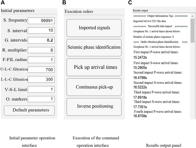
FIGURE 9. Basic function graphical user interface.

3.5.2 Signal analysis functions

The soft-signal analysis interface was mainly divided into three image areas, namely the original signal image area, the seismic phase recognition image area, and the arrival pickup image area. The original signal image area shows the waveform of the original signal obtained from the import data function, the seismic phase recognition image area is the seismic phase recognition result obtained from the seismic recognition function through the red dotted rectangular box, and the arrival pickup image area is the exact arrival time of the P-wave and the peak arrival time of the S-wave obtained from the pickup arrival function through the circle and the square, respectively.

3.5.3 Inverse positioning function

The inverse positioning interface was divided into four main functional areas, namely the optimization algorithm and objective function adjustment control, the geophone coordinates and the arrival time display and modification control, the initial parameters display and adjustment control, and the source inversion positioning image display and adjustment control. By entering the initial parameters such as the geophone coordinates, dual-phase arrival time, and the search starting point of the optimization algorithm, the inverse positioning function was used to locate the microseismic source inversion.

3.5.4 Other functions

To facilitate further analysis of the microseismic signals and a comparative analysis between different methods, the following functions are provided:

1) Optimization algorithms are available as pattern search algorithm, variable step accelerated search method, simulated annealing algorithm, and genetic algorithm.

2) The objective function could be selected as either single-phase or dual-phase, with two single-phase objective functions available under the single-phase option, and one dual-phase objective function corresponding to the dual-phase option.

3) The initial parameters and the geophone coordinates and the arrival support the function of modifying and restoring the default parameters.

4) The 3D plot window and the result output panel support clearing function.

5) The initial arrival time could be selected according to the single or double oscillation phase with only the P-wave precise arrival time or only the S-wave peak arrival time, or a corresponding group of the precise P-wave arrival time and the peak arrival time of the S-wave could be selected at the same time.

Some of the other features are shown in Figure 10.

FIGURE 10

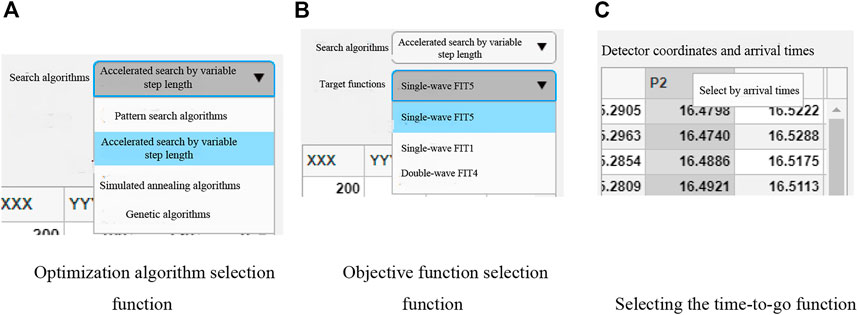
FIGURE 10. Display of some other functions.

4 Engineering example validation

4.1 Engineering validation of the seismic phase identification

According to the monitoring results of the ground monitoring station of the Tashan mine, the microseismic signals generated from seven microseismic events with different periods and different seismic locations were classified, and the sources were named as “Source I” to “Source O”, in which each event contained seven three-directional microseismic signals. Each event contained seven microseismic signals in the X-, Y-, and Z-axes, and each microseismic signal contained one microseismic response, and the signal form is shown in Figure 11.

FIGURE 11

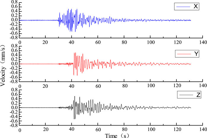
FIGURE 11. Schematic diagram of microseismic signal in microseismic monitoring project.

4.1.1 Comparison of the effect of seismic phase recognition

The initial parameters used for the adaptive rotational categorization method in the following analysis were: sampling frequency, F_s =5000 Hz, sampling interval, C_int =10, grouping interval, F_int =10 s, and range expansion factor, Q = 2.

1) Analysis of identification results

Through daily monitoring of the microseismic events in the mine area, a total of 168 microseismic signals were collected from seven sources, seven geophones, and three sub-directions, which were expressed in the form of “source - sub-direction”. For e.g. “I-X” indicates the microseismic signals from source I and the X-axis sub-direction of the geophone. The microseismic signal was monitored under source I (Liu et al., 2017). The results are shown in Figure 12, where each rectangle represents a segment of a microseismic signal, and the true value of microseismic response count of each segment was 1. If the result is 1, the recognition was classed under successful, and if not, the recognition was classed under failed. The absolute value of the difference between the number of phases and the true value of the microseismic response is called the recognition deviation.

FIGURE 12

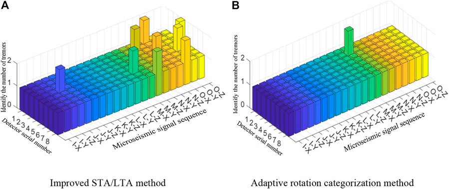
FIGURE 12. Microseismic phase identification results of the two methods.

From Figure 12A it can be seen that the number of recognition failures of the improved STA/LTA method is 9 times, the maximum magnitude of recognition bias is one time, and the distribution of recognition failure results is not regular. From Figure 12B it can be seen that the number of recognition failures of the adaptive rotational categorization method is one time, and the maximum magnitude of recognition deviation is one time.

2) Calculation time analysis

As shown in Figure 13, the calculation time of the improved STA/LTA method and the adaptive rotational categorization method was higher than that of the adaptive rotational categorization method for the above 168 segments of microseismic signals with a mean value of 0.281 s and a wide range of variation of 0.303 s. The calculation time of the adaptive rotational categorization method is shorter than that of the improved STA/LTA method, with a mean value of 0.115 s and a small range of variation of 0.152 s. The calculation time of the adaptive rotational categorization method is shorter than that of the improved STA/LTA method. and the range of computation time variation is also smaller, with a polar difference of 0.152 s.

3) Comparison of the recognition effect of the two methods

FIGURE 13

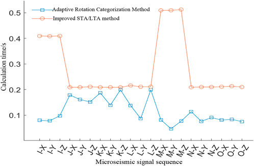
FIGURE 13. Calculation time for the two methods

By collating and analyzing the identification results with the computation time, the results are shown in Table 2.

TABLE 2

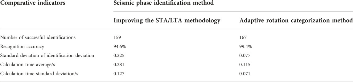
TABLE 2. Comparison of the microseismic phase identification effects for the two methods.

As can be seen from Table 2, compared with the improved STA/LTA method, the recognition accuracy of the adaptive rotational categorization method is improved by 4.8%, the standard deviation of recognition deviation is 34.2% of the former, the mean value of computation time is 40.9% of the former, and the standard deviation of computation time is 55.9% of the former. This shows that the method has advantages over the improved STA/LTA method in terms of seismic phase recognition accuracy, stability, and computation speed and stability, and thus has advantages over the improved STA/LTA method.

4.2 Engineering validation of the TFA-DC method

To further verify the reliability of the TFA-DC method for microseismic signal arrival pickup, the microseismic signal data from the microseismic monitoring project at the Tashan Mine were selected for verification, as shown in Figure 14, and the pickup results are shown in Table 3.

FIGURE 14

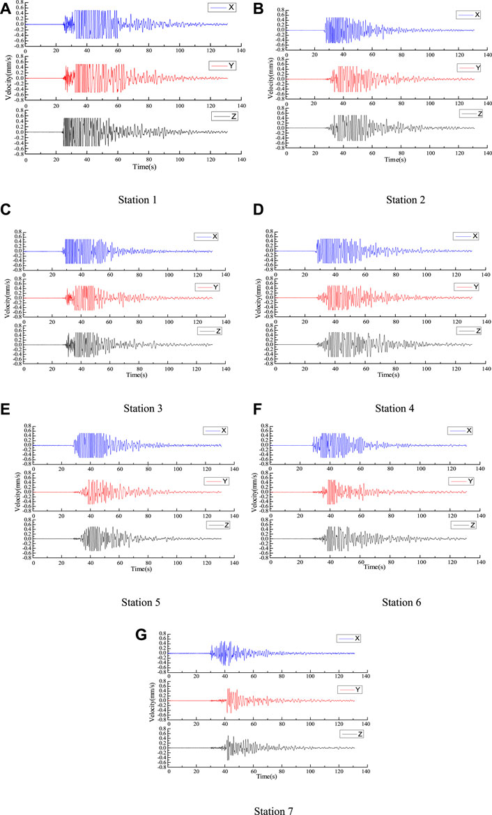
FIGURE 14. Three-component velocity profiles for each station for microseismic events.

TABLE 3

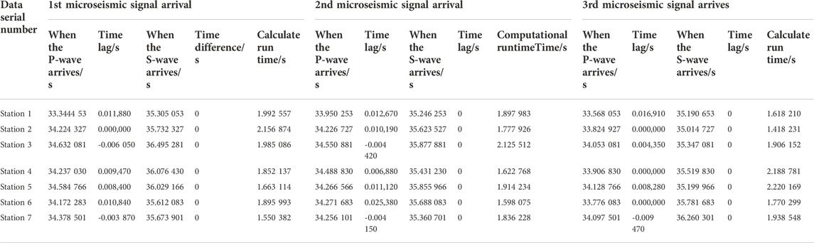
TABLE 3. Analysis of arrival-time picking results of data from the practical engineering by TFA-DC.

According to Table 3, the following conclusions can be drawn:

1) The maximum time difference, the minimum time difference, the mean time difference and the standard deviation of the time difference at the peak of the S-wave to time are all 0 s.

2) The maximum time difference when the P-wave is accurate is 0.025380 s, the minimum time difference is 0 s, the average time difference is 0.007825 s, and the standard deviation of the time difference is 0.006180 s.

3) The maximum calculated run time is 2.220,169 s, the minimum calculated run time is 1.418,231 s, the average calculated run time is 1.853,774 s, and the standard deviation of the calculated run time is 0.220,383 s.

4) There is no pickup failure due to low signal-to-noise ratio in the above pickup results.

It can be seen that the TFA-DC method has certain advantages in terms of the types of the pickup waves, the average time difference, the standard deviation of time difference, the average computation time required for a single pickup, the standard deviation of time, and the success rate of pickup. This indicates that it is an effective method for picking up microseismic signals in time, and can thus meet the needs of engineering sites.

4.3 Engineering example validation of the variable-step accelerated search method

In order to further demonstrate the advantages of the variable-step acceleration search method for seismic source localization, the localization effects of the three algorithms, the simulated annealing algorithm, the genetic algorithm, and the variable-step acceleration search method, were compared using the P-wave initial arrival time and the spatial coordinates of the geophone from engineering field data under the simplified velocity model using the average wave velocity.

4.3.1 Geophone coordinates and observation arrival times

The data obtained from blasting at the Tashan mine were used as an example to compare and analyze the positioning effects of the three algorithms. The first arrivals of the P-waves were picked up by the seven geophones after the blast, and the blast coordinates, i.e., the true values of the source, were determined at the site (2,732.7 m, 226,57.6 m, 56.3 m). The spatial coordinates of each geophone and the arrival times of the P-wave first arrivals picked up by them are shown in Table 4.

TABLE 4

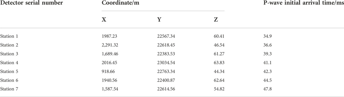
TABLE 4. Geophone coordinates and first arrival-time of the P-waves.

4.3.2 Analysis of the variable-step acceleration search method

To this end, the initial coordinates of the starting point were: X₀ = 1,000 m, one Y₀ = 20000 m, Z₀ = 30 m; the initial value of the average wave velocity of the P-wave, V₀ = 5 m/ms: the upper limit of the model size, X_u = 5000 m: Y_u = 30000 m: Z_u = 100 m: the lower limit of the model size, X_d = 0 m, Y_d = 0 m, Z_d = 0 m; the upper limit of the velocity, V_u = 20 m/s: the lower limit of the velocity, V_d = 0 m/s: the search step for the lower limit, J = 0.001 m: and the initial value of search step, r = 2000 m. The results of the 10 calculations using the variable-step acceleration search method are shown in Table 5.

TABLE 5

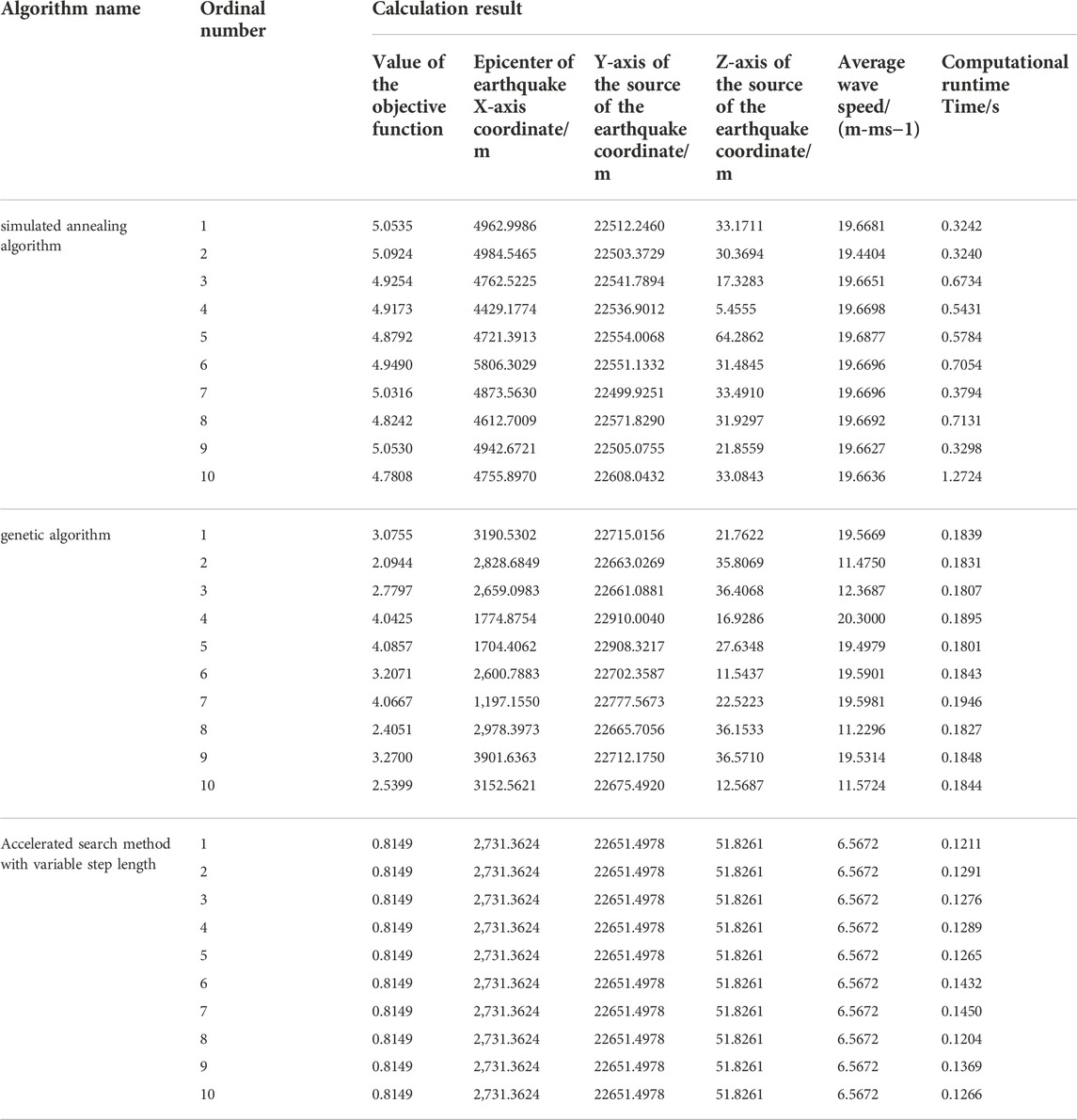
TABLE 5. The location results of the three algorithms.

Data shown in Tables 5 and 6 imply that the mean and standard deviation of the objective function value, and the mean and standard deviation of the localization error of the variable step acceleration search method are smaller than the remaining two algorithms. This indicates that the accuracy and convergence stability of the results of this algorithm were better than the remaining two algorithms, and the mean value of the computation time was smaller than the remaining two algorithms.

TABLE 6

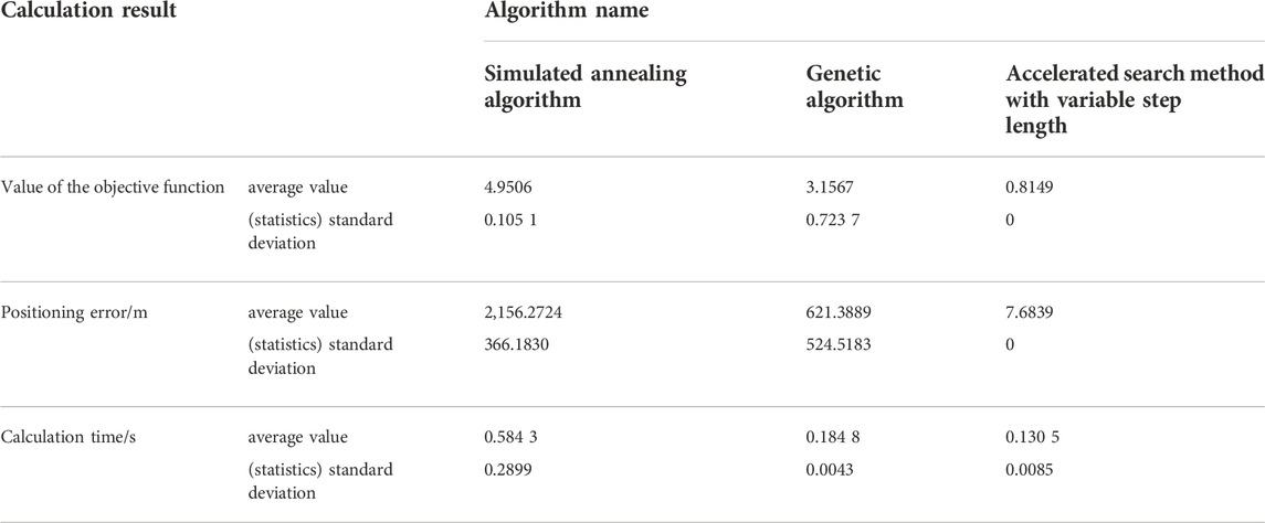
TABLE 6. Comparison of location effect of three algorithms.

Hence, the variable-step acceleration search method could find the optimal convergence point precisely and quickly with the specified P-wave arrival time, the target function model, and the coordinates of the geophones. and the results are guaranteed to be the same every time. The optimization algorithm had no substantial impact on the localization accuracy, which was mainly due to other factors such as P-wave arrival time, objective function model, geophone position coordinates, and wave speed model.

4.4 Engineering validation of the TD-DL methods

In order to further confirm the superiority and practicality of the TD-DL method in seismic-source inversion localization, the seismic signals from the microseismic monitoring project of the Tashan mine were selected for the on-time pickup and inversion localization calculation, and the results were compared with the localization calculation results of P-wave and S-wave single seismic phases. These signals were named as, “KZXH-1”, “KZXH-2”, and “KZXH-3”. The time pickups of the above three groups of microseismic signals were performed using the TFA-DC method, and the time pickups obtained after the filtering process are shown in Figure 15, and the obtained P-wave precise time pickups and S-wave peak time pickups are shown in Table 7.

FIGURE 15

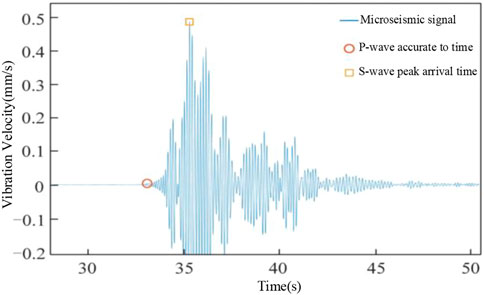
FIGURE 15. Schematic diagram of picking up mine seismic signal at arrival-time.

TABLE 7

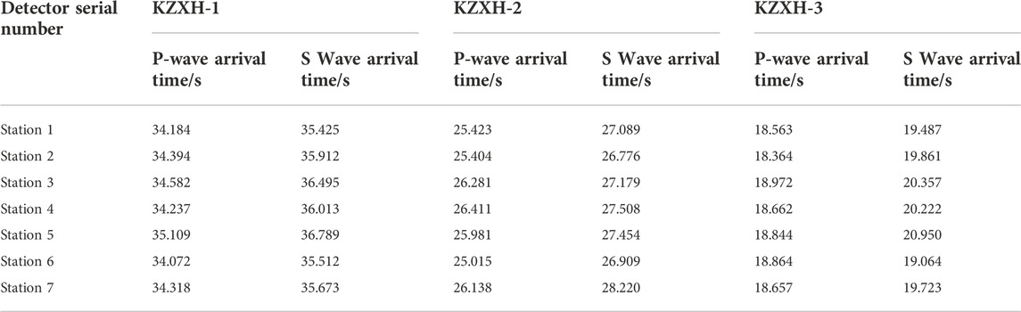
TABLE 7. Arrival-time data of P-wave and S-wave of mine seismic signal.

4.4.1 Geophone arrangement

The geophones of the mine microseismic monitoring project were arranged at a depth of 2 m below the surface, and were only used for two-dimensional monitoring, i.e., monitoring the X-axis and Y-axis coordinates of the source location, so the coordinate variation range of the geophones are mainly distributed in the X-axis and Y-axis, and its coordinates are shown in Table 8.

TABLE 8

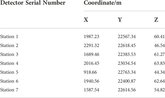
TABLE 8. Three-dimensional coordinates of the geophones at the

4.4.2 Analysis of positioning results

In order to increase the constraint information at the arrival of the double-shock phase and improve the convergence and positioning accuracy of the localization algorithm, the Z-axis coordinates were imported at the same time in addition to the geophone X-axis and Y-axis coordinates for cooperative localization during the calculation., and only the X-axis and Y-axis coordinates are used for the localization results. Although the variation range of the Z-axis coordinates of the geophones was much smaller than that of the X-axis and Y-axis, the addition of the Z-axis coordinates increased the convergence error tolerance and reduced the converged objective function value. This indicated that the addition of the Z-axis coordinates improved the positioning accuracy. After importing the geophone coordinates and arrival data, the inverse localization calculations were performed using the variable-step accelerated search method, and the results were compared with the true coordinates of each source and the localization errors are shown in Table 9, where the true coordinates of the source were obtained from the reported seismic location of the mine.

TABLE 9

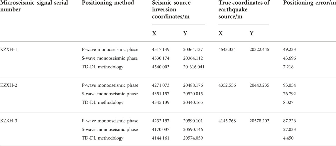
TABLE 9. Location results of each seismic phase in mine seismic signal.

From Table 9, it can be seen that under the source KZXH-1, the TD-DL method localization error is 14.7% and 16.5% of the P-wave and the S-wave single seismic phases, respectively; under the source KZXH-2, the TD-DL method localization error is 8.6% and 10.5% of the P-wave and the S-wave single seismic phases, respectively; under the source KZXH-3, the TD-DL method localization error is 5.1% and 16.5% of the P-wave and the S-wave single seismic phases, respectively.

4.5 Engineering applications of integration software

In January 2019, the high-frequency microseismic wireless ground monitoring system of Tashan coal mine was officially put into operation, and the monitoring was carried out during the operation of Tashan coal mine 8204–2 working face, which is an isolated island working face with the risk of power disaster. In April, the working face was advanced 120 m, and a total of 41 microseismic events were monitored, with a total release energy of 24,300 J, including 15 events below 102 J, 15 events between 102 J and 103 J, 12 events between 103 J and 104 J, and no events larger than 104 J. At this stage, the working face was widened, the advance speed was reduced, and the number of microseismic events and the energy of microseismic events were low.

The microseismic signal microseismic arrival time pickup and its localization were performed using the integrated software for microseismic events received at station one from 12:00 to 14:00 on April 10. From the integrated software, the microseismic arrival time and source location of the microseismic events in the mine was easily obtained. It was easy to operate and did not require complicated calculations. The process merely imported the measured microseismic waveform data by clicking on the arrival time pickup from the software, and the source inversion positioning to get the desired results. The obtained positioning data are shown in Table 10, and the positioning effect is shown in Figures 16, 17.

TABLE 10

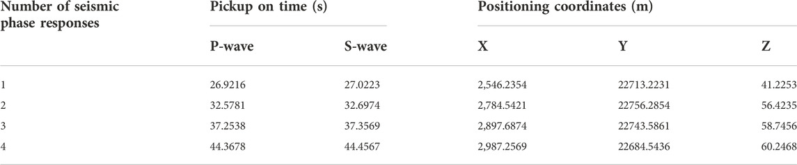
TABLE 10. Integrated software inversion of Tashan mine positioning data on April 10.

FIGURE 16

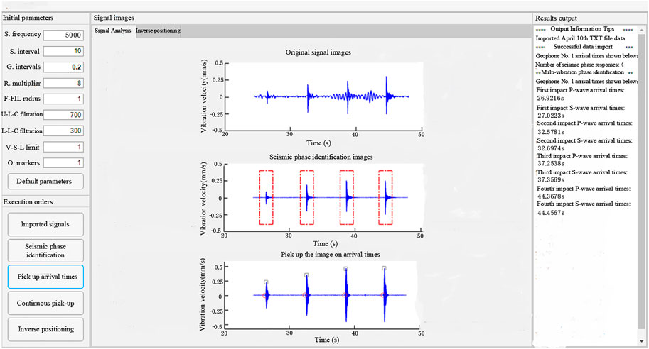
FIGURE 16. Software calculation of the April 10 microseismic arrival pickup event.

FIGURE 17

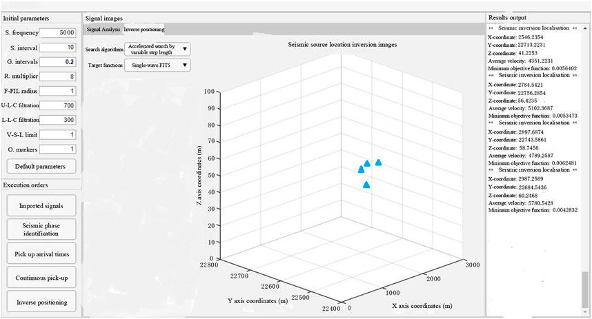
FIGURE 17. Software calculation of the microseismic localization results for the April 10 event.

5 Conclusion

Combining simulated algorithms, geophone coordinates, initial arrival times, and microseismic signals obtained from actual projects. The main conclusions that can be drawn are as follows:

1) Analysis of microseismic signals based on monitoring of isolated working face at Tashan mine, the recognition accuracy of the adaptive rotation categorization method improved by 4.8%, the standard deviation of recognition deviation was 34.2% of the former, and the mean and standard deviation of calculation time were 40.9% and 55.9% of the former, respectively.

2) The TFA-DC method compares with the improved STA/LTA method, the average time difference and the standard deviation of the former P-wave were 6.18‰ and 3.98‰ of the latter, the average computation time and standard deviation required for a single pickup of the former were 43.99% and 10.54% of the latter, and the former arrival time pickup failure ratio was 0, while for the latter was 15.63%.

3) Under the simulated cases, when simulated annealing algorithm and the genetic algorithm were compared, the standard deviation of the objective function value, the standard deviation of the localization error, and the standard deviation of the wave velocity error of the variable-step acceleration search method were all 0; the average value of the localization error of this algorithm was 0.7% and 1.9% of the remaining two.

4) The TD-DL method offset the positioning errors obtained from the P-wave and S-wave single-phase calculations to a certain extent, thus improving the inversion positioning accuracy of the source; the average value of the positioning errors of the TD-DL method under the engineering data was 9.5% and 14.5% of the P-wave and S-wave single-phase positioning, respectively.

5) The software was integrated with “visual”, “interactive” and “one-click” features for microseismic data processing, and the analysis of the April data from the Tashan mine enables faster and more direct access to the location of the source of microseismic events.

Data availability statement

The original contributions presented in the study are included in the article/supplementary material, further inquiries can be directed to the corresponding author.

Author contributions

The author confirms being the sole contributor of this work and has approved it for publication.

Funding

2020 Liaoning Provincial Education Department Scientific Research Funding Project (LJ2020JCL022).

Conflict of interest

The author declares that the research was conducted in the absence of any commercial or financial relationships that could be construed as a potential conflict of interest.

Publisher’s note

All claims expressed in this article are solely those of the authors and do not necessarily represent those of their affiliated organizations, or those of the publisher, the editors and the reviewers. Any product that may be evaluated in this article, or claim that may be made by its manufacturer, is not guaranteed or endorsed by the publisher.

References

Cui, F., Yang, Y. B., Lai, X. P., and Cao, J. T. (2019). Experimental study of physical similar materials based on microseismic monitoring key strata fracture induced rock burst. Chin. J. Rock Mech. Eng. 38 (4), 803–814. doi:10.13722/j.cnki.jrme.2018.1423

CrossRef Full Text | Google Scholar

Diehl, T., Deichmann, N., Kissling, E., and Husen, S. (2009). Automatic S-wave picker for local earthquake tomography. Bull. Seismol. Soc. Am. 99 (3), 1906–1920. doi:10.1785/0120080019

CrossRef Full Text | Google Scholar

Dong, L. J., Wesseloo, J., Potvin, Y., and Li, X. B. (2016). Discrimination of mine seismic events and blasts using the Fisher Classifier, Naive Bayesian Classifier and logistic regression. Rock Mech. Rock Eng. 49 (1), 183–211. doi:10.1007/s00603-015-0733-y

CrossRef Full Text | Google Scholar

Gong, S., Dou, L., Ma, X., Mu, Z. L., and Lu, C. P. (2012). Optimization of network layout algorithm for improving microseismic positioning accuracy in coal mine. Chin. J. Rock Mech. Eng. 31 (1), 8–17. https://kns.cnki.net/kcms/detail/detail.aspx?FileName=YSLX201201004andDbName=CJFQ2012

Google Scholar

Gong, S., Dou, L., Ma, X., and Liu, J. (2010). Selection of optimal number of channels to improve microseismic positioning accuracy in coal mine. J. China Coal Soc. 35 (12), 2017–2021. doi:10.13225/j.cnki.jccs.2010.12.014

CrossRef Full Text | Google Scholar

Jia, B., Jia, Z., Zhao, P., and Chen, Y. (2017). Microseismic localization in small scale region based on high-density array. Chin. J. Geotechnical Eng. 39 (4), 705–712. https://kns.cnki.net/kcms/detail/32.1124.tu.20160918.1242.004.html

Google Scholar

Jia, B., Li, F., Pan, Y., and Zhou, L. L. (2022). Microseismic source location method based on variable stepsize accelerated search. Rock Soil Mech. 43 (3), 843–856. doi:10.16285/j.rsm.2021.0872

CrossRef Full Text | Google Scholar

Jiang, R. C., Dai, F., Liu, Y., and Li, A. (2021). A novel method for automatic identification of rock fracture signals in microseismic monitoring. Measurement 175, 109129. doi:10.1016/j.measurement.2021.109129

CrossRef Full Text | Google Scholar

Lee, M., Byun, J., Kim, D., Choi, J., and Kim, M. (2017). Improved modified energy ratio method using a multi-window approach for accurate arrival picking. J. Appl. Geophys. 139 (1), 117–130. doi:10.1016/j.jappgeo.2017.02.019

CrossRef Full Text | Google Scholar

Li, J., Lei, W., Zhao, H., Wang, T., Liu, Y. H., and Zhang, H. (2019). Microseismic response characteristics of coal and rock impact failure under repeated blasting. J. China Univ. Min. Technol. 48 (5), 966–974. doi:10.13247/j.cnki.jcumt.001053

CrossRef Full Text | Google Scholar

Li, J., Zhang, H., Rodi, W. L., and Toksoz, M. N. (2013). Joint microseismic location and anisotropic tomography using differential arrival times and differential backazimuths. Geophys. J. Int. 195 (3), 1917–1931. doi:10.1093/gji/ggt358

CrossRef Full Text | Google Scholar

Li, L., He, C., and Tan, Y. (2017). Research on microseismic observation system and source location objective function. Acta Sci. Nat. Univ. Peking. 53 (2), 329–343. doi:10.13209/j.0479-8023.2016.091

CrossRef Full Text | Google Scholar

Li, N., Wang, E., Sun, Z., and Li, B. L. (2014). Source location method of simplex microseismic based on L1 norm statistics. J. China Coal Soc. 39 (12), 2431–2438. doi:10.13225/j.cnki.jccs.2013.1855

CrossRef Full Text | Google Scholar

Li, X., and Xu, N. (2020). Research status and prospect of microseismic source location. Prog. Geophys. 35 (2), 598–607. https://kns.cnki.net/kcms/detail/11.2982.P.20190624.1628.197.html

Google Scholar

Liu, X., Zhao, J., Wang, Y., and Peng, P. A. (2017). Microseismic P-wave automatic picking technology based on improved STA/LTA method. J. Northeast. Univ. Nat. Sci. Ed. 38 (5), 740–745. https://kns.cnki.net/kcms/detail/detail.aspx?FileName=DBDX201705028andDbName=CJFQ2017

Google Scholar

Pan, Y., Zhao, Y., Guan, F., Li, G. Z., and Ma, Z. S. (2007). Research and application of seismic monitoring and positioning system. Chin. J. Rock Mech. Eng. 26 (5), 1002–1011. https://kns.cnki.net/kcms/detail/detail.aspx?FileName=YSLX200705020andDbName=CJFQ2007

Google Scholar

Perol, T., Gharbi, M., and Denolle, M. (2018). Convolutional neural network for earthquake detection and location. Sci. Adv. 4 (2), e1700578. doi:10.1126/sciadv.1700578

PubMed Abstract | CrossRef Full Text | Google Scholar

Ross, Z. E., Meier, M. A., and Hauksson, E. (2018). P-wave arrival picking and first-motion polarity determination with deep learning. J. Geophys. Res. Solid Earth 123 (6), 5120–5129. doi:10.1029/2017jb015251

CrossRef Full Text | Google Scholar

Tian, Y., and Chen, X. (2002). Review on seismic location. Prog. Geophys. 17 (1), 147–155. https://kns.cnki.net/kcms/detail/detail.aspx?FileName=DQWJ200201023andDbName=CJFQ2002

Google Scholar

Wang, H., Liang, M., and Zhu, M. (2020). Hybrid localization algorithm of microseismic source based on simplex and shortest path ray tracing. China Min. Ind. 29 (10), 110121–111115. https://kns.cnki.net/kcms/detail/detail.aspx?FileName=ZGKA202010019andDbName=CJFQ2020

Google Scholar

Wang, Y-H., Wang, B-l., and Duan, J-H. (2019). Microseismic location based on differential evolution algorithm. Coal Geol. Explor. 47 (1), 168–173. https://kns.cnki.net/kcms/detail/detail.aspx?FileName=MDKT201901026andDbName=CJFQ2019

Google Scholar

Wu, S. J., Wang, Y. B., Zhan, Y., and Chang, X. (2016). Automatic microseismic event detection by band-limited phase-only correlation. Phys. Earth Planet. Interiors 261, 3–16. doi:10.1016/j.pepi.2016.09.005

CrossRef Full Text | Google Scholar

Xue, Q., Wang, Y., and Chang, X. (2018). Joint inversion of location, excitation time and amplitude of microseismic sources. Bull. Seismol. Soc. Am. 108 (3A), 1071–1079. doi:10.1785/0120170240

CrossRef Full Text | Google Scholar

Zhao, C., Tang, S., Qin, M., Guo, X. Q., Jiao, W. Y., and Liu, C. (2019). Experimental study on positioning accuracy of microseismic monitoring system. Min. Technol. 19 (2), 46–49. doi:10.13828/j.cnki.ckjs.2019.02.015

CrossRef Full Text | Google Scholar

Zhao, G. Y., Ju, M. A., Dong, L. J., Li, X. b., Chen, G. h., and Zhang, C. x. (2015). Classification of mine blasts and microseismic events using starting-up features in seismograms. Trans. Nonferrous Metals Soc. China 25 (10), 3410–3420. doi:10.1016/s1003-6326(15)63976-0

CrossRef Full Text | Google Scholar

Zheng, Y., Wang, Y., and Chang, X. (2016). Wave equation based microseismic source location and velocity inversion. Phys. Earth Planet. Interiors 261, 46–53. doi:10.1016/j.pepi.2016.07.003

CrossRef Full Text | Google Scholar