Automatic karst cave detection from seismic images via a convolutional neural network and transfer learning

The identification of karst caves in seismic imaging profiles is a key step for reservoir interpretation, especially for carbonate reservoirs with extensive cavities. In traditional methods, karst caves are usually detected by looking for the string of beadlike reflections (SBRs) in seismic images, which are extremely time-consuming and highly subjective. We propose an end-to-end convolutional neural network (CNN) to automatically and effectively detect karst caves from 2D seismic images. The identification of karst caves is considered as an image recognition problem of labeling a 2D seismic image with ones on caves and zeros elsewhere. The synthetic training data set including the seismic imaging profiles and corresponding labels of karst caves are automatically generated through our self-defined modeling and data augmentation method. Considering the extreme imbalance between the caves (ones) and non-caves (zeros) in the labels, we adopt a class-balanced loss function to maintain good convergence during the training process. The synthetic tests demonstrate the capability and stability of our proposed network, which is capable of detecting the karst caves from the seismic images contaminated with severe random noise. The physical simulation data example also confirms the effectiveness of our method. To overcome the generalization problem of training the neural network with only synthetic data, we introduce the transfer learning strategy and obtain good results on the seismic images of the field data.

Introduction

Carbonate reservoir plays an important role in oil and gas exploration due to its characteristics of high yield, large scale, and high quality of crude oil and gas (Gao et al., 2016). Many efforts have been made to study the prediction and characterization of the carbonate-karst reservoirs (Loucks 1999; Qi and Yun, 2010; Chen et al., 2011; He et al., 2019). Traditional methods such as seismic attributes are generally applied to detect carbonate-karst reservoirs. Trani et al. (2011) present a 4D seismic inversion scheme of AVO and time-shift analysis to predict the pressure and fluid saturation changes in reservoirs. Ma et al. (2014) propose a strategy to estimate the stable elastic parameters from prestack seismic data and demonstrate its application by making predictions of the carbonate gas reservoir in the Sichuan Basin. Li et al. (2014) apply the residual signal matching tracing method to improve the lateral resolution of the top boundary of small-scale carbonate reservoirs, restore the shape of the SBRs, and help to identify small-scale reservoirs in limestone. Liu and Wang (2017) use seismic discontinuities, seismic facies classification, stochastic inversion, and lithofacies classification to detect faults and karst fractures in the carbonate reservoir. Lu et al. (2018) apply the discrete frequency coherence attributes to detect the fractured-vuggy bodies in carbonate rocks. Dai et al. (2021) propose a high-precision multi-scale curvature attribute to detect carbonate fractures. The improvement of the traditional curvature solving algorithm improves the accuracy of curvature calculation. These studies only focus on the prediction of the entire carbonate reservoirs, rather than the characterization and prediction of the karst caves. However, accurate cave detection is extremely important for finding high-quality reservoirs and well placement since they are rich in oil and gas.

Complex diagenesis usually makes the karst cave structures extremely developed in carbonate rocks. He et al. (2019) propose an accumulation energy difference method to directly identify karst caves using the seismic reflection energy in trace or between traces. Sun (2018) develops a multi-scale karst cave detection method based on prestack frequency division and migration imaging and then demonstrates its application with the field data in Tahe oilfield. However, the direct detection of karst caves in carbonate fracture-cavern reservoirs is challenging, since the troditional methods do not treat the caves separately, but identify them together as part of the oil and gas reservoir collective. These reservoir identification methods are less accurate for identifying caves. Generally, the dissolution caves appear as string of beadlike reflections (SBRs) on the seismic migration profiles, which are considered as an indicator for high-quality reservoirs (Wang et al., 2017). Correct detection and extraction of SBRs from seismic imaging profiles are helpful for quantitative description of karst cave reservoirs. Wang et al. (2017) propose a tensor-based adaptive mathematical morphology to extract the SBRs from seismic images and remove the effects of seismic events and noise. These conventional methods cannot cleanly extract the SBRs from seismic images nor accurately depict the karst cave positions. Besides, they are computationally expensive and rely heavily on human intervention. Therefore, there is an interest to develop a more efficient, robust, and accurate karst cave detection technique.

Recently, deep learning has been widely used in geophysics to solve some practical problems, such as velocity model building (Yang and Ma, 2019), denoising (Yu et al., 2019; Wang et al., 2022), first arrival picking (Yuan et al., 2018; Hu et al., 2019; Yuan et al., 2022), and seismic trace interpolation (Wang et al., 2020). Wu et al. (2019) propose an end-to-end neural network for automatic fault detection, which is regarded as a binary segmentation problem. The binary labels consist of zeros (non-faults) and ones (faults). The network trained only with the synthetic data set is applied directly to the field data set and achieves a relatively good fault detection. In this study, we consider karst cave detection as an image recognition problem of labeling a 2D seismic image with ones on caves and zeros elsewhere. We focus on the automatic karst cave detection directly from seismic images using a modified U-Net. We add a boundary padding operation into each convolutional layer to make the input and output of the same size. Because the binary label is highly unbalanced between ones (caves) and zeros (non-caves), a class-balanced cross-entropy loss function is introduced to ensure that the gradient of the network descends in the correct direction during the training process. We develop an automatic modeling method for building velocity models with karst caves and generate the synthetic imaging profiles through convolution. The diffraction points with different scales and velocities are used to simulate the karst caves and the velocity models with cavities are generated by randomly adding the diffraction points to the velocity models. We apply data augmentation such as noise addition, resampling, and vertical rotation around the depth axis to the synthetic data to improve the diversity of the training data set. Then the well-trained network is tested with the synthetic seismic images contaminated with random noise. We also validate its capability of karst cave detection with physical simulated data. Before applying the trained network to the field data, we introduce transfer learning to strengthen the network and bridge the gap between the field data and synthetics. The field data tests demonstrate the generalization ability of the updated network.

During the training stage, the neural network takes in the seismic images and effectively learns the nonlinear relationship between the imaging profiles and the binary images. Although the training process is computationally expensive, the cost of the prediction is negligible once the network training is completed. With an NVIDIA RTX5000 GPU, our neural network takes less than 1 s to identify karst caves from 2D seismic images.

Training data sets

To train an efficient network, a large amount of training data set and the corresponding labels are required. However, labeling caves manually is time-consuming and highly dependent on human intervention, which may sometimes lead to incorrect labels. Inaccurate labeling including unlabeled and mislabeled caves may affect the training process of the neural network and decrease the detection accuracy of the trained network. To address these issues, we develop an automatic and effective method to establish the velocity models with karst caves and create the corresponding seismic images.

Automatic velocity model generation

To generate the training and testing data sets, we first establish a certain number of velocity models without karst caves through an automatic modeling strategy inspired by the data augmentation method for automatic fault segmentation in Wu et al. (2019). As is shown in Figure 1, the velocity models are designed in four types, including horizontal layered models with velocity gradually increased with depth (A), curved layered models with velocity gradually increased with depth (B), models featured with thick and reverse layers (C), and models with a high-speed anomaly (D). In this workflow, we first create the horizontal layered velocity models with different layers. The velocity values of each layer range from 2,000 to 6,500 m/s. All the automatically generated velocity models have the same size of 700 × 350 points and the spatial interval is 20 M. Then, we increase the complexity by vertically shearing the velocity model. 20 velocity models randomly cropped from the Marmousi model are added into the training data set to increase model complexity. A total of 100 velocity models are automatically generated during this process.

FIGURE 1

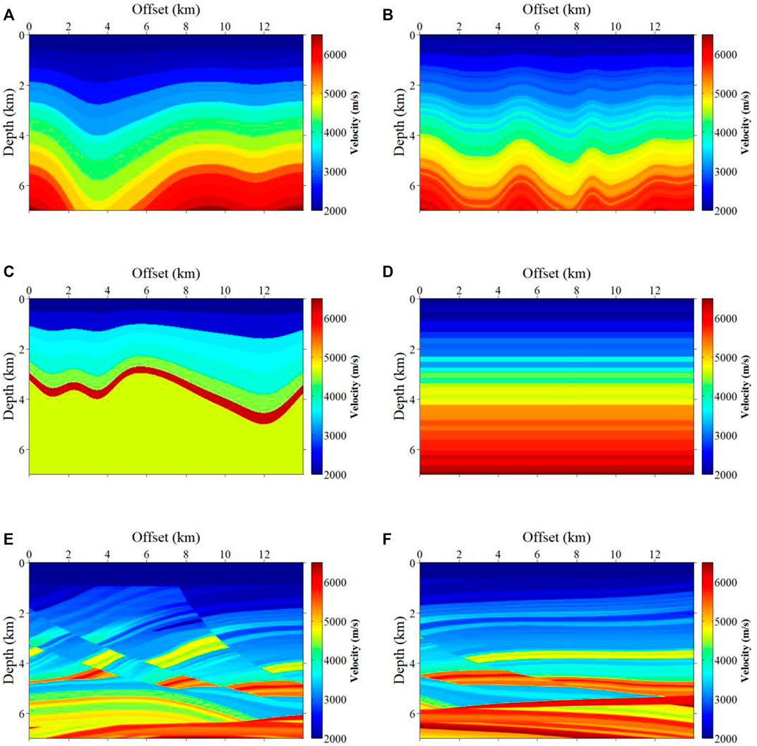
FIGURE 1. Six representative self-generated velocity models with different geological structures. (A) represents the horizontal layered models; (B) refers to the curved layered models; (C) denotes the models featured with thick and reverse layers; (D) is the models with a high-speed anomaly. (E) and (F) represent the cropped section from the Marmousi model.

Adding diffraction points

We simulate the velocity models with karst caves by adding different scales of diffraction points to the velocity models. The diffraction points are designed as 1 × 1, 2 × 2, and 3 × 3 to simulate different scales of cavities. There are two main reasons why we chose to use a square to simulate a cave. One is that a square is more convenient in modeling, the other is that we analyzed the field data to be predicted and found that the cave is relatively small on the migration images and its shape can be approximated as a square. A total of 150 diffraction points with different velocities and scales are randomly added to each velocity model. The velocity values of the caves shift from −0.3 to −0.5 times to the original velocity values. Figure 2 shows six representative velocity models with karst caves (colored squares). The corresponding binary labels consisting of zeros (non-caves) and ones (caves) are shown in Figure 3.

FIGURE 2

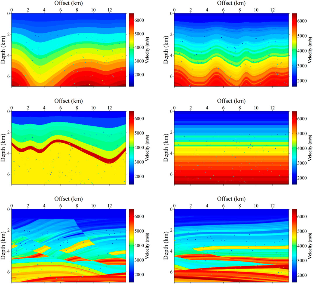
FIGURE 2. Six representative velocity models with karst caves, which are generated by adding diffraction points (colored squares) to the velocity models in Figure 1.

FIGURE 3

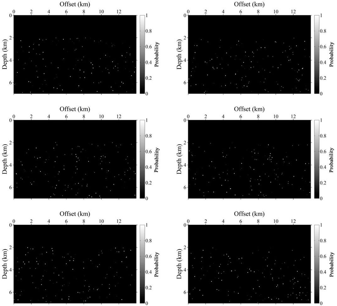
FIGURE 3. Six labels correspond to the velocity models with karst caves in Figure 2. The white spots in the binary images denote karst caves (ones) and the elsewhere black area represents non-karst caves (zeros).

Seismic image generation

We focus on automatically detecting the karst caves from 2D seismic imaging profiles. The network is trained by seismic images generated from the velocity models with cavities, and the output is a 2D distribution probability map of karst caves. Considering the differences between the field seismic records and the simulated seismic data derived with wave equation forward modeling, we obtain the corresponding seismic images by convolution to generate the input data set, which greatly reduces the computational cost compared with the traditional imaging method. We first transform the velocity models into reflectivity models and then obtain the seismic images by convolving the Ricker wavelet with the reflectivity models. The peak frequency of the Ricker wavelet is randomly chosen in a limited range we defined. We add random noise to the convolutional results to simulate more realistic seismic images. Figure 4 shows the final 2D seismic images obtained from the corresponding velocity models with karst caves in Figure 2. It shows that the seismic images derived by convolution and noise addition are very similar to the field data. The diversity of the training samples is increased, which is crucial to successfully train an effective karst cave detection network.

FIGURE 4

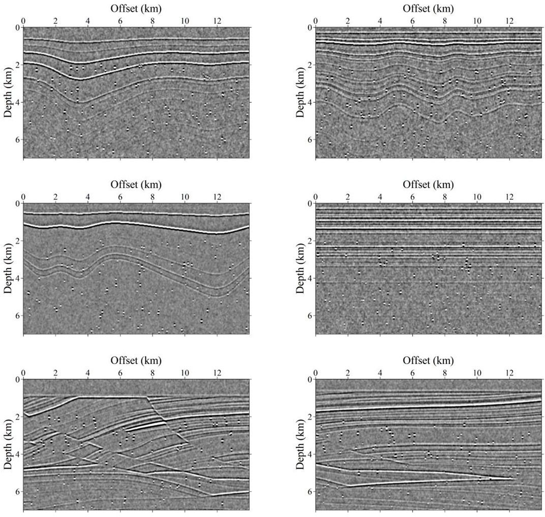
FIGURE 4. The corresponding seismic images generated by convolution. Random noise is added to make the seismic data more realistic.

CNN-based karst cave detection method

In this section, we first introduce the network architecture for karst cave detection in detail. Then, a class-balanced binary cross-entropy loss function (Xie and Tu, 2015) is illustrated.

Network architecture

We perform karst cave identification by modifying the original U-net architecture (Ronneberger et al., 2015), which is proved to be effective for detecting the cavities from seismic images. Figure 5 illustrates the detailed convolutional neural network (CNN), in which an input 2D seismic image is fed into the network that consists of a contracting path (left) for extracting the cave features and an expansive path (right side) for accurate cave detection. As is shown in Figure 5, each step in the left contracting path includes two 3 × 3 convolutional layers, followed by a ReLU activation and a 2 × 2 max-pooling operation with a stride of two for downsampling. The ReLU activation can make the output of some neurons be 0, resulting in the sparsity of the network and alleviating the occurrence of over-fitting problems. The max-pooling operation compresses the features and reduces the calculation of the training and prediction. Symmetrically, each step on the right expansive path contains a 2 × 2 upsampling operation and two 3 × 3 convolutional layers followed by a ReLU activation. The upsampling is conducted by nn. convtranspose2d in the PyTorch module. In each step, the concatenation path links the left and right paths to recover the spatial information destroyed mainly by max-pooling and other operations. The sigmoid activation function in the last convolutional layer is to produce a probability map of the output with the same size as the input. The main body of our network is similar to that of the original U-Net architecture and a total of 23 convolutional layers are included in this network.

FIGURE 5

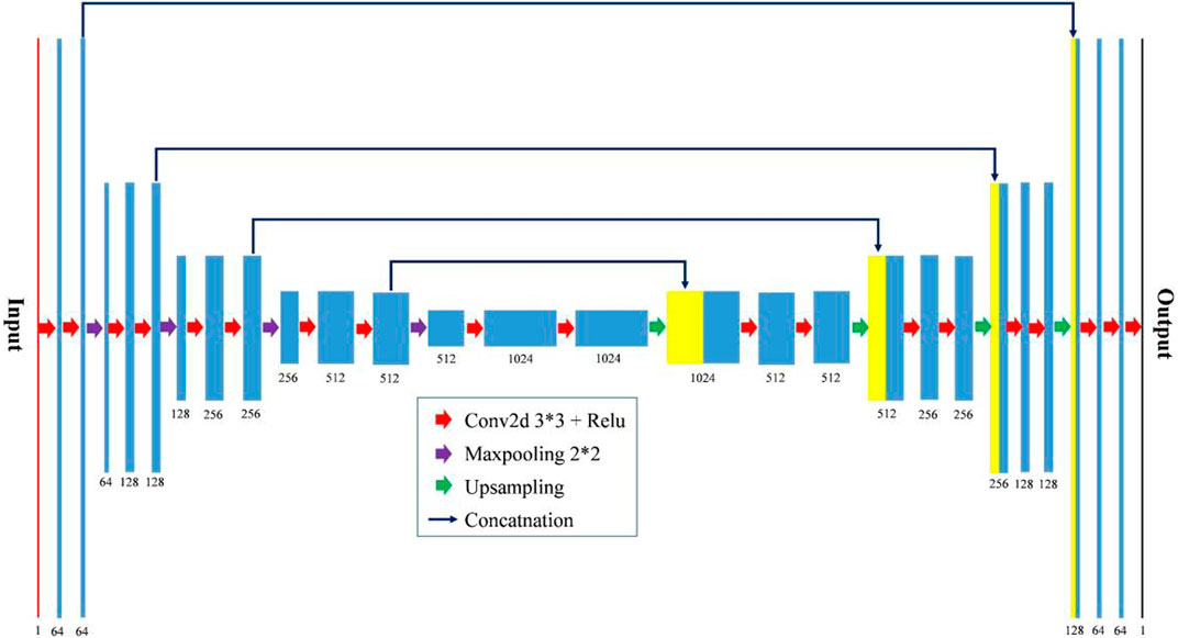
FIGURE 5. The proposed symmetrical convolutional neural network (U-Net) for automatic karst cave recognition.

Class-balanced cross-entropy loss

The loss function calculates the differences between the labels and the predictions. For a binary segmentation problem, the following binary cross-entropy loss function is widely adopted:

$\mathrm{L}\mathrm{o}\mathrm{s}\mathrm{s}=-{\displaystyle \sum }_{i=1}^n\left(y_i\times \ln x_i+\left(1-y_i\right)\times \ln \left(1-x_i\right)\right)(1)$

where n is the number of pixels in the input 2D seismic image. $y_i$ is the true binary labels (0 or 1) and $x_i$ denotes the prediction probabilities ($0{<y}_i<1$) calculated from the sigmoid activation in the last convolutional layer. This binary cross-entropy loss function is suitable to the common dichotomy problems, in which the distribution of zeros and ones in the label is generally balanced. However, it works not well for our karst cave detection problem, in which most samples are non-cave samples (labeled by zeros), whereas the proportion of caves (ones) is relatively small. With this loss function, the network may make zero predictions everywhere to make the loss value very small, making the network converge in the wrong direction. To address this problem, a class-balanced binary cross-entropy loss function (Xie and Tu, 2015) is introduced to solve the imbalance so that the network is not trained or converged to predict only zeros.

$\mathrm{L}\mathrm{o}\mathrm{s}\mathrm{s}=-{\displaystyle \sum }_{i=1}^n\left(\beta \times y_i\times \ln x_i+\left(1-\beta \right)\times \left(1-y_i\right)\times \ln \left(1-x_i\right)\right)(2)$

where $\beta =Y_0/Y$ and $1-\beta =Y_1/Y$ . $Y_0$ and $Y_1$ are the number of pixels of caves and non-caves in the label data set, respectively. $Y$ denotes the total number of pixels in the label data set. Using the class-balancing weight $\beta$ on a per-pixel term basis, the binary cross-entropy loss with additional trade-off parameters for biased sampling helps the network converge in the correct direction.

Training and testing

We generate a total of 100 seismic images and the corresponding labels, then we divide the inputs into 5,000 sample patches in total using data augmentations. We first crop a random area in these seismic images, and then resample it to a fixed size, e.g. 64 $\times$ 64 points. We assign 4,500 and 500 samples as the training and validation data sets, respectively. Figure 6 shows four representative samples of the training data set. The first column denotes the velocity models, the second column represents the corresponding seismic images as inputs, and the third column is the karst cave probability distribution maps as the labels. The training data set is crucial to train an effective karst cave detection network. During the training process, we apply data augmentation such as flip horizontal to improve the diversity of the training data set. For each input of the seismic image, we first rotate the seismic profiles by 180° around the depth axis. We choose not to perform the rotation around the center point of the seismic profiles because it may destroy the inherent characteristic of vertical SBRs. Then, we enlarge each training data in a certain proportion and randomly crop the data with the size of 64 × 64 for the final inputs to further enhance data diversity.

FIGURE 6

FIGURE 6. Four representative samples of the training data set. The first column is the velocity models, the second column represents the corresponding seismic images as inputs, and the third column shows the karst cave probability distribution maps as the labels.

We focus on the identification of karst caves through image features and the relative numerical values. To balance the differences in numerical values between the inputs and improve the convergence of training, we normalize the input seismic images. Many factors such as the learning rate, batch size, and training epoch can greatly affect the detection performance of this neural network. During the training process, data is transmitted to the network in batch form and the selection of batch size depends on the problem to be solved. For data with complex features and large sample differentiation, the larger batch size can effectively avoid the destruction of network convergence by discrete samples but reduce the training efficiency of the network exponentially. For the single feature recognition problem with obvious features, the smaller batch is a better choice. We focus on the identification of karst caves by SBRs on seismic images via CNN, which is a simple feature identification problem. The batch size is set to be eight to balance training efficiency and ensure correct convergence. We take the Adam method (Kingma and Ba, 2014) as the optimization strategy of the network parameters and set the learning rate to be 0.0001. We train the network with 100 epochs, and all the 4,500 seismic images are processed at each epoch. Figure 7 shows the convergence curves of the training (red line) and validation (green line) data sets. With the increase of the number of iterations, the prediction accuracy is improved, while the convergence curve of the validation data set decreases to a certain extent and then stops decreasing. It indicates that the network trained with the training data set has achieved the best effect on the validation data set and the continuous training may lead to overfitting. The outputs of the network are probabilities ranging from 0 to 1, and we set the threshold to 0.5. i.e., all output values greater than 0.5 are considered as caves, which is equivalent to a probability of 1. Conversely, for all output values less than 0.5, after thresholding, all are considered as non-caves.

FIGURE 7

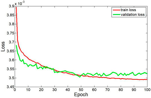
FIGURE 7. The training and validation loss decrease with epochs.

Numerical experiments and applications

In this section, we first test the proposed network with synthetic data, including the seismic data with noise-free and the seismic images with random noise. Then we apply the network trained with only synthetics to the physical simulated data set of integrated geological models. Finally, we perform karst cave identification on the field data based on transfer learning.

Predictions on the synthetic data set

We first test our network with synthetic data without noise. We select the partial BP 2.5D model and the complete Marmousi model as two basic models for generating the validation data set. We establish two corresponding velocity models with karst caves by the same cave simulation method. Figures 8A,B show the partial BP 2.5D model and the Marmousi model with karst caves, both of which contain a total of 150 caves. Figures 8C,D represent the corresponding seismic images obtained by convolution with the Ricker wavelet. It shows that each karst cave in the velocity model corresponds to a clear SBR on the seismic images. The energy of SBRs produced by each cave is different since the velocity differences between the caves and the surrounding rocks are different. When the velocity differences between the karst caves and surrounding rocks are small, the energy of the corresponding SBRs is weak. Figures 8E,F are the overlaid images of the prediction results (red spots) and the seismic images in Figures 8C,D. The results show that the trained network can accurately identify every karst cave. It recognizes the SBRs with weak energy as well as the close or adherent karst caves. It indicates that the prediction accuracy can be 100% for the seismic images without noise. Here we define the accuracy as the percentage of caves identified divided by the number of total caves. Note that the training data set includes the seismic images with random noise, which demonstrates that the recognition ability of the network to the normal SBRs is not affected by the addition of random noise to the training data set. The trained network can make accurate predictions for the SBRs embedded in the reflective layer, which are likely to be ignored in traditional interpretation. This is reasonable because the input of the network is a 2D array with specific values rather than figures. Although the SBRs on the seismic images are contaminated by the reflective layer, the numerical values prove the existence of SBRs. The trained neural network can not only identify the karst caves but also predict their scales and positions since the true locations and scales of the caves are included in the label. The CNN network takes the strong reflected energy in the upper left of the Marmousi model that is similar to the SBRs on a single trace, as non-cave. Considering that the karst caves on a small scale are actually distributed sporadically, we assume the karst caves to be cubes when generating the data set. Therefore, the trained network can not recognize the long beaded energy clusters that extend laterally as a cave.

FIGURE 8

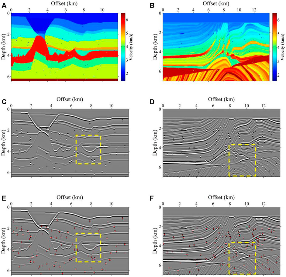
FIGURE 8. The prediction results on the testing data set. (A) The partial BP 2.5D model with karst caves. (B) The Marmousi model with karst caves. (C,D) The corresponding seismic images of (A,B). (D–F) The overlaid images, consisting of the predicted karst caves of the trained neural network (red spots) and seismic images (C,D).

Then we verify the capability of the proposed network with seismic images contaminated with random noise. The two velocity models in Figures 9A,B are the same as in Figure 8. We add random noise to the convolution results (Figures 9C,D). Not only the SBRs of weak energy are almost covered by the noise, but the SBR characteristics of the strong energy are destroyed. The predicted results in Figures 9E,F indicate that the trained network can correctly identify most karst caves. Under the noise interference, the network predicts the cave accuracy of BP 2.5D model and Marmousi model with 92% and 90%, respectively. The addition of Gaussian random noise can destroy the original distribution characteristics of the SBRs or cover the weak SBRs, rather than forging a bead-like energy cluster. The presence of noise can affect the imaging results and lead to degradation of image quality. For some tiny caves or caves with minor difference in velocity between the internal fill and the surrounding rock, its SBR features may be covered or destroyed, resulting in the network not being able to identify it correctly, since SBR is the basis for the network to identify the caves. However, the presence of noise does not lead to similar SBR or false SBR on the imaging results. Therefore, in this case, the network will not recognize some small caves, but it will not increase the recognition error rate. Therefore, the trained network may fail to recognize the karst caves but not misidentify them. A-D and E-H in Figure 10 are the enlarged display of the yellow dotted box in Figures 8, 9, respectively. Figures 10A,B,E,F are the enlarged display of the seismic images and prediction results of the BP 2.5D model. There are fewer reflective layers and the distance between the adjacent reflective layers is large. The comparison between Figures 10B,F show that the SBRs of the unrecognized karst caves in the noise case are completely contaminated by the noise, which cannot be identified by the features or the numerical values. The right four subfigures in Figure 10 correspond to the enlarged view of the Marmousi model, which contains many thin layers and complex structures. The karst caves are distributed in the thin layers or faults. Figures 10D,F indicate that the karst caves in which the SBR energy is drowned by random noise are not recognized by the neural network. The SBRs with weak energy close to the complex structures are not identified by the trained network since the SBRs are damaged by the noise. Figures 10F,H show that some SBRs whose energy is submerged or the SBRs are destroyed by noise can still be accurately predicted by the trained network. This is because the velocity difference between the cave and the surrounding rock is large, which represents a diffraction wave with strong energy in the seismic records, and then presents as a strong energy cluster in the imaging profiles. The trained neural network can make predictions by searching for the energy anomalies, such as the high energy of the SBR center and by the vertical imaging features.

FIGURE 9

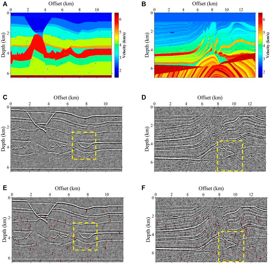
FIGURE 9. The prediction results on the testing data set with random noise. The symbols are the same as in Figure 8.

FIGURE 10

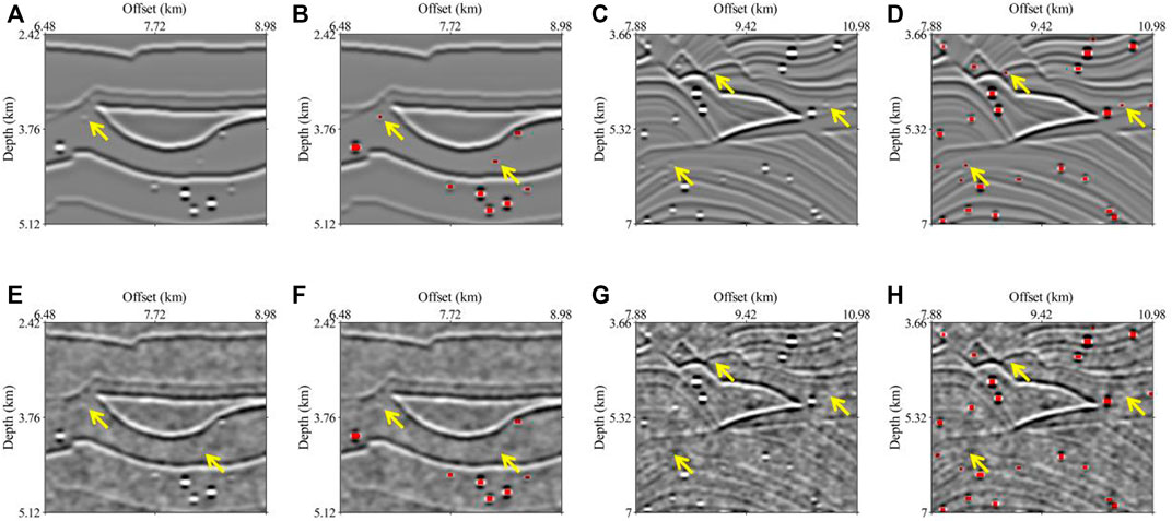
FIGURE 10. An enlarged view of the area selected by the yellow dotted line in Figure 9 and Figure 8.

Predictions on physical simulated data

Before applying the proposed method to the field data, we first test the trained network with a physical simulated data set, which is derived by the physical simulation of an integrated geological model. The physical model is created by casting in three dimensions, including an undulating overburden, karst caves, riverway, and faults. The karst caves of different scales and depths are simulated by cubes made of specific materials. The generated training data set is based on the assumption that the caves are square, which is similar to the simulated karst caves in the physical model. Therefore, this physical simulation data is suitable to validate this method. There is a horizontal parallel target layer beneath the overlay strata containing various geological structures. As shown in Figure 11, the red line denotes the upper rugged surface of the overlay strata, the purple squares represent the karst caves with different scales and depths, and the green area is the target layer. The whole model is placed in the tank and is supported by the gasket at the bottom. An excitation transducer and a receiving transducer are both placed above the water tank as a source to transmit ultrasonic waves to the water and as a geophone to receive the signal, respectively.

FIGURE 11

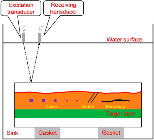
FIGURE 11. The physical simulated model, and ultrasonic data excitation and collection system.

We apply the network trained with only synthetics to the imaging profiles of the physical simulated data to verify the capability of this method. Figure 12A is an imaging profile on the crossline, including three karst cave clusters with different arrangements and depths. Figure 12B shows the predicted results overlaid with Figure 12A. It shows that the network trained with synthetic data can make predictions on the imaging results of physical simulated data. Although the characteristics of the SBRs are different from the synthetic data, and the migration noise is different from the added Gaussian noise, the proposed network can effectively identify caves through the energy intensity and the vertical energy distribution of the SBRs. Figure 13A shows the migration results of the inline, in which the karst caves with gradually increasing burial depths are distributed on the left side, and the scattered caves and the cross-sections of the riverway are distributed on the right side. The prediction results (Figure 13B) indicate that the trained network can make accurate recognition for karst caves with different burial depths, and the predicted cave positions are consistent with the central energy of the SBRs. The scattered karst caves embedded in the riverway are accurately predicted by the neural network. The pseudo-beading features in the middle of the model are not misidentified as karst caves.

FIGURE 12

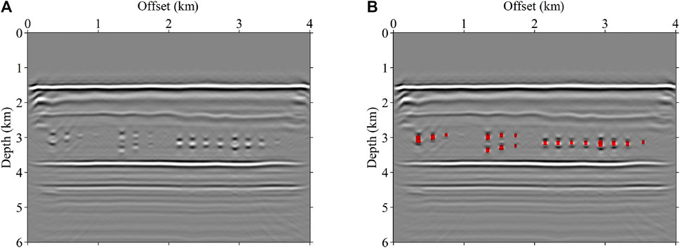
FIGURE 12. The imaging results and prediction results of the physical simulated data on the crossline section. (A) is the seismic image, and (B) is the overlaid display of (A) and the predicted results.

FIGURE 13

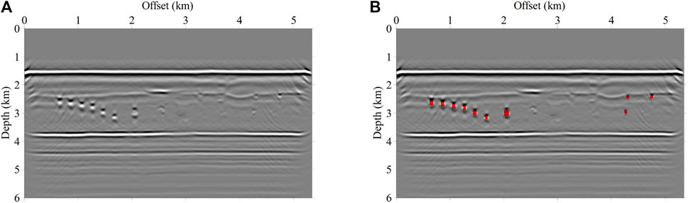
FIGURE 13. The imaging results and prediction results of the physical simulated data on the inline section. (A) is the seismic image, and (B) is the overlaid display of (A) and the predicted results.

Predictions on field data

Finally, we validate the detection ability of the trained network with the field data. The imaging results of the field data are complicated and differ greatly from the synthetics, which makes the network trained with only synthetic data unable to identify karst caves accurately. Transfer learning is an effective way to bridge the gap between field data and synthetics. For two domains with similar features, transfer learning enables the neural network to transfer the detection ability learned with massive training data to the domain that the training data is difficult to obtain, which is shown to be effectively applied to the field data. We select four sections from the imaging results of the field data and recognize the karst caves manually. Then we generate the training data according to the four imaging profiles and the corresponding karst cave interpretation results. Finally, 200 training samples are generated using the same data processing method, and are fed into the network at the 101 epoch to continue training. We only update the parameters of the last convolutional layer to complete the transfer of the network to the field data. This allows the network to retain the weights previously trained on the synthetic data sets. For the main body of the network, which is the encoder-decoder structure, it has the ability to identify caves according to the SBR. We only train the last convolutional layer of the network with the new training data to transfer its cave recognition capability to the field data. Then we apply the updated network to the migration results of the field data.

Figures 14, 15 are the imaging results (A and D) and the corresponding prediction results (C and F) on the crossline and inline sections, respectively. Meanwhile, we performed manual cave picking for these four profiles, and the results of human identification are shown Figures 14B,E and Figures 15B,E. Although the SBRs in the seismic images of the field data are different from the synthetics, the updated network can effectively identify karst caves from the field data through transfer learning. For some small SBRs with weak energy, the updated network can also make accurate detection. Figure 14A shows that the karst caves are densely developed in the middle and bottom, and the imaging features are messy due to the complex geological structure. The corresponding predicted results in Figure 14C demonstrate that the updated network is capable of detecting such adjacent karst caves. Figure 14D corresponds to the migration imaging result of another survey line on the crossline section, in which the overall energy of the SBRs is weak. As is shown in Figure 14F, almost all the karst caves are accurately identified, and the positions of the predicted karst caves are consistent with the central energy of the SBRs. Comparing Figures 14B,C, the results of human identification and network prediction are basically consistent, and the network can distinguish better in the areas where small caves are densely developed. For the profile in Figure 14D, the number of manually identified caves is less than that predicted by the network. For a series of laterally arranged karst caves in the shallow area of Figure 15A, the network can make accurate predictions and separate them well without sticking together (Figure 15C). Figure 15D shows that there are three distinct SBRs, and some SBRs with weak energy, and a large SBR that extends laterally in the shallow part. The corresponding predicted results in Figure 15F indicate that the network can accurately predict the karst caves from the conventional SBRs and can make effective karst cave detection from the shallow SBRs after transfer learning. For both profiles in Figure 15, some small caves as well as the caves where SBR is not obvious, the trained network has an advantage. In conclusion, the benefits of the network is that it can detect some weak SBRs and thus predict the caves, which may be ignored by human fast identification. In terms of efficiency, using convolutional neural networks to predict caves is advantageous compared to manual recognition.

FIGURE 14

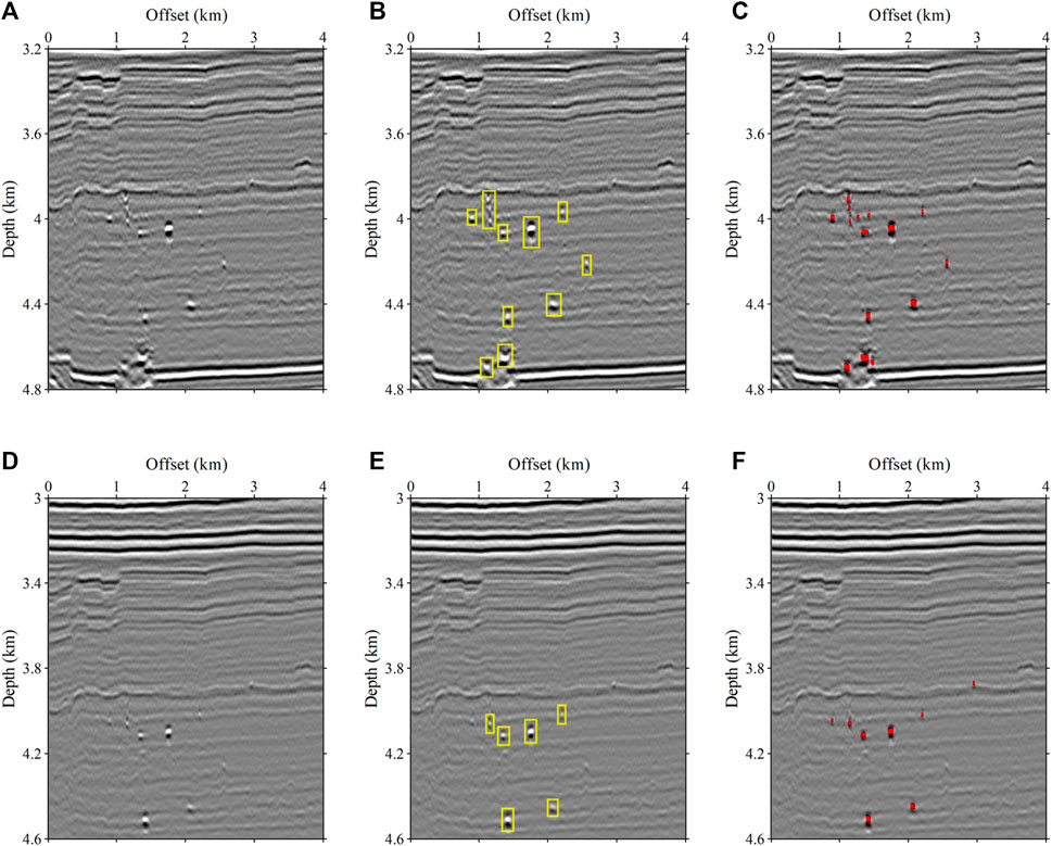
FIGURE 14. The imaging results and prediction results of the physical simulated data on the crossline section. (A) and (D) are the seismic images. (B) and (E) are the manually cave picking results. (C) and (F) are the overlaid display of seismic images and the predicted results.

FIGURE 15

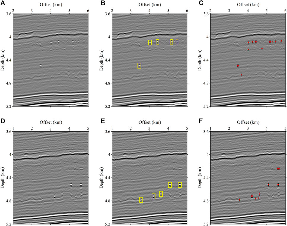
FIGURE 15. The imaging results and prediction results of the physical simulated data on the inline section. The symbols are the same as in Figure 14.

Discussion

We validate the capability of this proposed neural network for karst cave detection through synthetic data. The network trained with only synthetics can be applied to the testing data set generated by convolution. The trained network can make completely accurate predictions from the seismic images with noise-free. For the imaging results contaminated with random noise, the trained network can identify most of the karst caves. A few caves are not successfully recognized because the SBRs are destroyed by noise, which can also not be identified by manual interpretation. We apply the trained network directly to the imaging profiles of the physical simulation data and achieve accurate predictions, which demonstrates its generalization ability. This is because the seismic recordings of the physical simulation data have a high signal-to-noise ratio (S/Ns) and the karst caves in the physical simulated model are all cubes of different scales, which is consistent with the assumptions of karst caves in our training data set generation. However, the migration imaging results of field data are messy and noisy since the actual geological situation is complex and the S/Ns of the shot records is low. Besides, the SBRs greatly differ from the synthetic data set because the underground karst caves are not cubes. By introducing transfer learning, the neural network can be applied to the imaging profiles of the field data and achieve accurate identification. It indicates that the neural network can be trained with the synthetic data first, which can be generated quickly and can be strengthened by transfer learning before applying it to the field data. For the reservoirs with complex fractures and karst cave development mechanisms, the proposed network cannot make effective identification because limited by seismic resolution, the imaging features are messy and no SBRs are presented. Whereas for the scattered SBRs, especially for the karst caves under the high-speed layer or the velocity differences with the surrounding rock are small, the energy of SBRs is weak, our neural network is capable of making accurate detection. This is important for interpretation because it helps interpreters to identify karst caves that are difficult to find or even missed.

The generated training data set is based on the assumption that the karst caves are cubes, while the actual karst caves are various kinds of shapes, not just cubes. For further improvement of this method, the simulation of caves with various shapes may improve the prediction accuracy of the network and have a better application on the field data. Besides, finite-difference modeling method and migration imaging can produce more realistic data sets, which should also improve the generalization ability of the network, if the computational cost is acceptable. With the more accurate simulation method, the trained network should have a better prediction ability in the reservoirs with complex fractures and karst cave development mechanisms.

Conclusion

We propose an end-to-end CNN to automatically and effectively identify karst caves directly from seismic imaging results, in which karst cave detection is regarded as a binary classification problem. We design a modeling method for automatically establishing velocity models and generating the synthetic training data through convolution. Data augmentation such as noise addition, resampling, and rotation are applied to the synthetic data to train an efficient network. Although trained with only synthetics, the neural network can effectively and accurately detect karst caves from seismic images contaminated with random noise, in which the SBRs of weak energy are covered by the noise or the SBR features of the strong energy are destroyed. The numerical example and physical simulated data demonstrate the capability and effectiveness of the proposed neural network for karst cave detection. The trained network is applied to the field data through transfer learning and makes accurate predictions.

Data availability statement

The raw data supporting the conclusion of this article will be made available by the authors, without undue reservation.

Author contributions

YH and JH contributed to the idea and methodology, YH was responsible for the training data production, model and field data testing, and the writing of this manuscript, BL assisted in testing the code, and YM checked and polished the manuscript. All authors have read the manuscript and agreed to publish it.

Funding

This research is supported by the National Key R&D Program of China under contract number 2019YFC0605503C, the Major projects during the 14th Five-year Plan period under contract number 2021QNLM020001, the National Outstanding Youth Science Foundation under contract number 41922028, the Funds for Creative Research Groups of China under contract number 41821002 and the Major Scientific and Technological Projects of CNPC under contract number ZD 2019-183-003.

Acknowledgments

The authors are grateful to the editors and reviewers for their review of this manuscript. Meanwhile, the authors would like to thank the PyTorch platform for providing excellent deep learning tools.

Conflict of interest

The authors declare that the research was conducted in the absence of any commercial or financial relationships that could be construed as a potential conflict of interest.

Publisher’s note

All claims expressed in this article are solely those of the authors and do not necessarily represent those of their affiliated organizations, or those of the publisher, the editors and the reviewers. Any product that may be evaluated in this article, or claim that may be made by its manufacturer, is not guaranteed or endorsed by the publisher.

References

Chen, M. S., Zhan, S. F., Wan, Z. H., and Zhang, H. Y. (2011). “Detecting carbonate-karst reservoirs using the directional amplitude gradient difference technique,” in Annual international meeting (San Antonio, Texas: SEG Expanded Abstracts), 1845–1849. doi:10.1190/1.3627564

CrossRef Full Text | Google Scholar

Dai, J. F., Li, H. Y., Zhang, M. S., Qin, D. H., and Xiao, S. G. (2021). “Application of multi-scale curvature attribute in carbonate fracture detection in caofeidian area, bohai bay basin,” in First international meeting for applied geoscience & energy (Denver, Colorado, USA: SEG, Expanded Abstracts), 1176–1180. doi:10.1190/segam2021-3583137.1

CrossRef Full Text | Google Scholar

Gao, Y., Shen, J. S., He, Z. X., and Ma, C. (2016). Electromagnetic dispersion and sensitivity characteristics of carbonate reservoirs. Geophysics 81 (5), E377–E388. doi:10.1190/geo2015-0588.1

CrossRef Full Text | Google Scholar

He, J. J., Li, Q., Li, Z. J., and Lu, X. B. (2019). Accumulative energy difference method for detecting cavern carbonate reservoir by seismic data. Geophys. Prospect. Pet. 48 (4), 337–341.

Google Scholar

Hu, L. L., Zheng, X. D., Duan, Y. T., Yan, X. F., Hu, Y., and Zhang, X. L. (2019). First-arrival picking with a U-net convolutional network. Geophysics 84 (6), U45–U57. doi:10.1190/geo2018-0688.1

CrossRef Full Text | Google Scholar

Kingma, D. P., and Ba, J. L. (2014). Adam: A method for stochastic optimization. https://arxiv.org/abs/1412.6980.

Google Scholar

Li, C., Gao, Y. F., Zhang, H. Q., and Wang, H. B. (2014). “Identification of small-scale carbonate reservoira,” in CPS/SEG Beijing 2014 International Geophysical Conference, 1312–1315. doi:10.2516/ogst/2021019

CrossRef Full Text | Google Scholar

Liu, Y., and Wang, Y. H. (2017). Seismic characterization of a carbonate reservoir in Tarim Basin. Geophysics 82 (5), B177–B188. doi:10.1190/geo2016-0517.1

CrossRef Full Text | Google Scholar

Loucks, R. G. (1999). Paleocave carbonate reservoirs: Origins, burial-depth modifications, spatial complexity, and reservoir implications. AAPG Bull. 83 (11), 1795–1834. doi:10.1306/E4FD426F-1732-11D7-8645000102C1865D

CrossRef Full Text | Google Scholar

Lu, Y. J., Cao, J. X., He, Y., Gan, Y., and Lv, X. S. (2018). “Application of discrete frequency coherence attributes in the fractured-vuggy bodies detection of carbonate rocks,” in CPS/SEG International Geophysical Conference, Beijing, China, 812–816. doi:10.1190/IGC2018-198

CrossRef Full Text | Google Scholar

Ma, J. Q., Geng, J. H., and Guo, T. L. (2014). Prediction of deep-buried gas carbonate reservoir by combining prestack seismic-driven elastic properties with rock physics in Sichuan Basin, southwestern China. Interpretation 2 (4), T193–T204. doi:10.1190/int-2013-0117.1

CrossRef Full Text | Google Scholar

Qi, L. X., and Yun, L. (2010). Development characteristics and main controlling factors of the Ordovician carbonate karst in Tahe oilfield. Oil Gas Geol. 31 (1), 1–12. doi:10.1130/abs/2020AM-358611

CrossRef Full Text | Google Scholar

Ronneberger, O., Fischer, P., and Brox, T. (2015). “U-Net: Convolutional networks for biomedical image segmentation,” in International Conference on Medical Image Computing and Computer-Assisted Intervention, Cham, 234–241. doi:10.1007/978-3-319-24574-4_28

CrossRef Full Text | Google Scholar

Sun, Z. (2018). Multi-scale cave detection based on amplitude difference of prestack frequency division. Geophys. Prospect. Petroleum 57 (3), 452–457. doi:10.3997/2214-4609.201801601

CrossRef Full Text | Google Scholar

Trani, M., Arts, R., Leeuwenburgh, O., and Brouwer, J. (2011). Estimation of changes in saturation and pressure from 4D seismic AVO and time-shift analysis. Geophysics 76 (2), C1–C17. doi:10.1190/1.3549756

CrossRef Full Text | Google Scholar

Wang, S. W., Song, P., Tan, J., He, B. S., Wang, Q. Q., and Du, G. N. (2022). Attention-based neural network for erratic noise attenuation from seismic data with a shuffled noise training data generation strategy. IEEE Trans. Geosci. Remote Sens. 60, 1–16. doi:10.1109/tgrs.2022.3197929

CrossRef Full Text | Google Scholar

Wang, Y., Lu, W. K., Wang, B. F., Chen, J. J., and Ding, J. C. (2017). Extraction of strong beadlike reflections for a carbonate-karst reservoir using a tensor-based adaptive mathematical morphology. J. Geophys. Eng. 14, 1150–1159. doi:10.1088/1742-2140/aa76d0

CrossRef Full Text | Google Scholar

Wang, Y. Y., Wang, B. F., Tu, N., and Geng, J. H. (2020). Seismic trace interpolation for irregularly spatial sampled data using convolutional autoencoder. Geophysics 85 (2), V119–V130. doi:10.1190/geo2018-0699.1

CrossRef Full Text | Google Scholar

Wu, X. M., Liang, L. L., Shi, Y. Z., and Fomel, S. (2019). FaultSeg3D: Using synthetic data sets to train an end-to-end convolutional neural network for 3D seismic fault segmentation. Geophysics 84 (3), IM35–IM45. doi:10.1190/geo2018-0646.1

CrossRef Full Text | Google Scholar

Xie, S. N., and Tu, Z. W. (2015). Holistically-nested edge detection. Int. J. Comput. Vis. 125, 3–18. doi:10.1007/s11263-017-1004-z

CrossRef Full Text | Google Scholar

Yang, F. S., and Ma, J. W. (2019). Deep-learning inversion: A next-generation seismic velocity model building method. Geophysics 84 (4), R583–R599. doi:10.1190/geo2018-0249.1

CrossRef Full Text | Google Scholar

Yu, S. W., Ma, J. W., and Wang, W. L. (2019). Deep learning for denoising. Geophysics 84 (6), V333–V350. doi:10.1190/geo2018-0668.1

CrossRef Full Text | Google Scholar

Yuan, S. Y., Liu, J. W., Wang, S. X., Wang, T. Y., and Shi, P. D. (2018). Seismic waveform classification and first-break picking using convolution neural networks. IEEE Geosci. Remote Sens. Lett. 15 (2), 272–276. doi:10.1109/lgrs.2017.2785834

CrossRef Full Text | Google Scholar

Yuan, S. Y., Zhao, Y., Xie, T., Qi, J., and Wang, S. X. (2022). SegNet-based first-break picking via seismic waveform classification directly from shot gathers with sparsely distributed traces. Petroleum Sci. 19 (1), 162–179. doi:10.1016/j.petsci.2021.10.010

CrossRef Full Text | Google Scholar