 Yuanshi Tian
 Jun Zhu1,2*
 Yusha Zhu
94% of researchers rate our articles as excellent or good
Learn more about the work of our research integrity team to safeguard the quality of each article we publish.
Find out more
ORIGINAL RESEARCH article
Front. Earth Sci., 25 January 2023
Sec. Solid Earth Geophysics
Volume 10 - 2022 | https://doi.org/10.3389/feart.2022.1042353
This article is part of the Research TopicChallenges and New Advances in Unconventional Resources ExploitationView all 6 articles
With the increase in the scale of mining in horizontal and highly deviated wells, electromagnetic boundary detection while drilling plays an important role in boundary detection. This paper examines three types of antenna structures commonly used in electromagnetic boundary detection and measurement methods and also performs a numerical simulation of the edge detection capability of the three structures in horizontal wells. The simulation experiment analyzes the influence of formation resistivity contrast, frequency, spacing, and other factors on the capability of edge detection and provides data that supports the design of instrument antenna parameters. The numerical simulation shows that the tilted and orthogonal receiving antennas demonstrate improved performance both in detecting the interface when approaching from high-resistance layers and low-resistance layers. In addition, the capability of boundary detection can be improved by decreasing the frequency and increasing the spacing between the transmitter and receiver.
In recent years, as the field of oil and gas exploration and development has transferred from structural reservoirs to unconventional reservoirs, the difficulty in oil and gas exploration has continued to increase. Expanding the detection range and enhancing the capability of boundary detection are necessary approaches to furthering understanding of active geological guidance and fine reservoir characterization (Clegg et al., 2022). Thus, electromagnetic boundary detection LWD technology has emerged.
Conventional LWD electromagnetic logging tools adopt single-transmitting and dual-receiving antennas, symmetrically compensated dual-transmitting and dual-receiving antennas, or multiple-transmitting and multiple-receiving array antennas (Nikitenko et al., 2020; Rodney et al., 1983; Clark et al., 1988; Bittar et al., 1991; Zhou et al., 2016; Fan et al., 2019). All transmitting and receiving antennas are axial, which means that they cannot measure azimuth information. In most cases, the spacing between transmitters and receivers is less than 1 m and the frequency ranges from hundreds of kilohertz to a few megahertz, which limits the capability of edge detection. One type of electromagnetic boundary detection logging tool, Schlumberger’s Periscope and Geosphere, uses a tilted antenna (Li et al., 2005; Omeragic et al., 2006; Antonsen et al., 2014; Seydoux et al., 2014; Zhu et al., 2021; Wu et al., 2022). The other type, by AziTrak and ViziTrak of Baker Hughes, uses an orthogonal antenna (Bell et al., 2006; Wang et al., 2007; Fang et al., 2008; Rabinovich et al., 2011). According to the detection range, EM boundary detection LWD tools can be divided into the azimuthal electromagnetic resistivity LWD tool (Hawkins et al., 2015) and the ultra-deep azimuthal electromagnetic resistivity LWD detection logging tool (Wu et al., 2019; Nemushchenko et al., 2022; Zhu et al., 2022).
Based on an investigation of existing electromagnetic boundary detection LWD tools, this paper conducted a numerical simulation on the edge detection capability in horizontal wells of three basic antenna unit structures. The transmitting antennas in the three structures were axial, and the receiving antennas were axial, tilted, and orthogonal. This paper also analyzes the influence of the formation resistivity contrast, frequency, spacing between transmitter and receiver, and other factors on the edge detection capability and provides data support for the design of the parameters of the instrument antenna.
The structure of electromagnetic boundary detection LWD tools with a single transmitter and single receiver in a horizontal well is shown in Figure 1A ; (x, y, z) is the horizontal well borehole coordinate system, z is the well axis direction, and (x', y', z') is the instrument coordinate system. When the instrument rotates around the well axis, the angle between the two coordinate systems is the azimuth angle
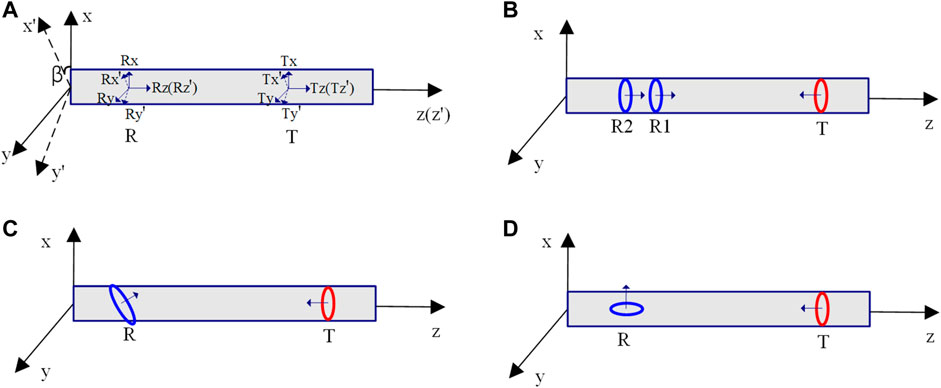
FIGURE 1. Schematic of the electromagnetic wave boundary detection instrument while drilling in the horizontal well.
In the borehole coordinate system, the magnetic field component generated by the transmitting and receiving antennas in different directions is H, wherein
According to the coordinate axis transformation theory (Wu et al., 2019), the magnetic field tensor H′ in the instrument coordinate system can be obtained as
Then, the magnetic field strength H′ in the instrument coordinate system is
Axial single-transmitting and dual-receiving antennas are the basic units of conventional LWD electromagnetic resistivity-logging tools (Rodney et al., 1983; Zhou et al., 2016) as shown in Figure 1B. The antenna system is comprised of an axial transmitting coil T and two receiving coils R1 and R2. The spacings from T to R1 and T to R2 are L1 and L2, respectively, wherein L2 > L1. The amplitude ratio (
An axial single-transmitting and tilted single-receiving antenna is the basic unit commonly used in Schlumberger azimuthal electromagnetic logging tools as shown in Figure 1C. The tilted coil receives both the
The received signal of the instrument changes the cosine with the azimuth angle
The axial transmitting and orthogonal receiving antenna is the basic antenna unit, which is used in instruments, such as AziTrak and VisiTrak (Bell et al., 2006; Rabinovich et al., 2011), as shown in Figure 1D. Using this antenna structure, the cross-coupled component signal
For EM boundary detection LWD tools, edge detection is aimed at detecting the radial boundary in horizontal and highly deviated wells. The formation model is simplified as a one-dimensional N-layer horizontal formation as shown in Figure 2. If the formation interface is curved, then it can be divided into multiple ideal states for superposition simulation. The thickness of the ith layer is
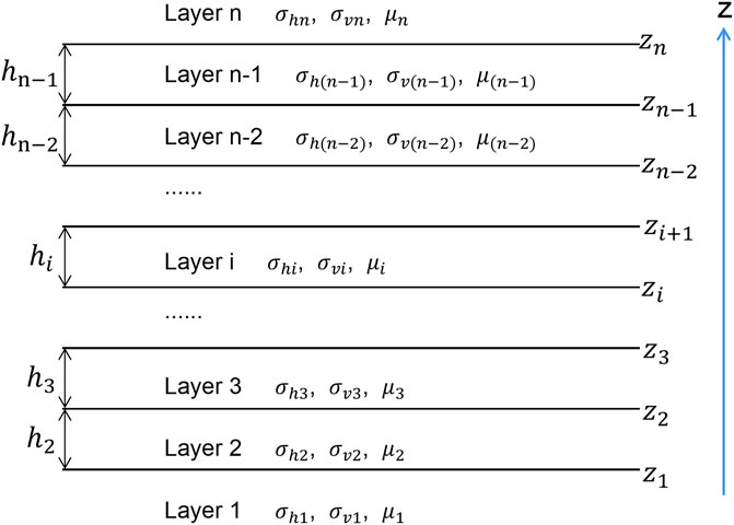
FIGURE 2. Model of the 1D N-layer horizontal layered formation.
For EM boundary detection LWD tools, the antenna size is considerably smaller than the distance between the transmitter and receiver; thus, the transmitting antenna is a magnetic dipole. The magnetic dipole in any direction can be decomposed into the superposition of the horizontal magnetic dipole (HMD) and the vertical magnetic dipole (VMD) (Chew, 1990; Wang et al., 2021). The transmitting antennas of the three aforementioned antenna structures all occur in the z direction. Therefore, only the magnetic field generated by VMD is considered below.
Introducing the magnetic Hertz potential (Moran and Gianzero, 1979; Bai et al., 2020; Li H. et al., 2020; Li K. et al., 2020; Hu et al., 2020), the VMD can be expressed as
where i in the subscript represents the field of the ith layer, and t indicates that the emission source is at the tth layer. The position of the transmitter T is
The magnetic field intensity generated by VMD in layered media is derived as follows.
where
The boundary conditions of the generated VMD are shown as follows:
When the transmitter is above the receiver,
When the transmitter is below the receiver,
Hankel integral transformation can be used to solve the integral formula Eq. 12, which contains the Bessel function (Anderson, 1979).
where
Fast Fourier–Hankel transform (FFHT) converts the integral operation of the Bessel function into a summation operation, which markedly simplifies the calculation and improves the operation speed. Moreover, the filter coefficient must only be calculated once (Li et al., 2018). Therefore, the algorithm has good calculation speed and stability.
Before conducting the calculations, the horizontal well formation model is established, as shown in Figure 3. Under the conditions of a single interface horizontal well, the distance between the formation interface and the instrument is the DTB. The DTB is altered to calculate its continuous response characteristics.
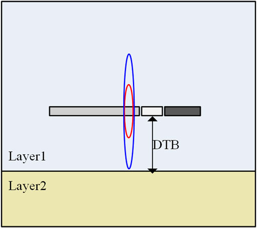
FIGURE 3. Simulation formation model of the EM boundary logging tool in the horizontal well.
The interface is located at DTB = 0, DTB >0 is formation 1, and DTB <0 is formation 2. The formation model parameters are shown in Table 1. The spacing between the transmitter and receiver is 1 m and the frequency is 100 kHz. Then, the boundary detection characteristics of three antenna structures, namely, the axial, tilted, and orthogonal receiver, are investigated.
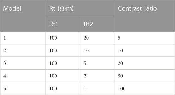
TABLE 1. Stratum model parameters.
The measured response EATT and
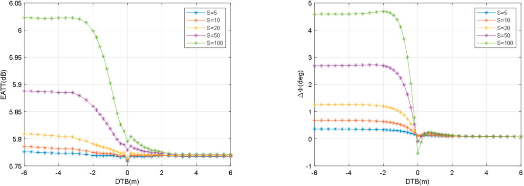
FIGURE 4. Response of the axial receiver in different contrast ratio stratum models.
The measured responses ATT and PS of the tilted receiving antenna are shown in Figure 5. The figure reveals that the ATT and PS curves of the five models nearly approach 0 when they are far away from the interface, which cannot quantify the formation resistivity. When approaching the interface, ATT and PS gradually increase and reach a maximum at the interface, and thus strengthen as the resistivity contrast ratio increases. ATT and PS can predict the presence of the interface at 2.4 m and 2 m near the interface at a high contrast ratio. However, ATT is less than 0.02 dB and cannot accurately measure the interface at a low contrast ratio (5 and 10). The edge detection capability of PS is better than ATT. Compared with conventional electromagnetic logging, the tilted antenna can accurately predict the formation interface even in a high resistivity layer.
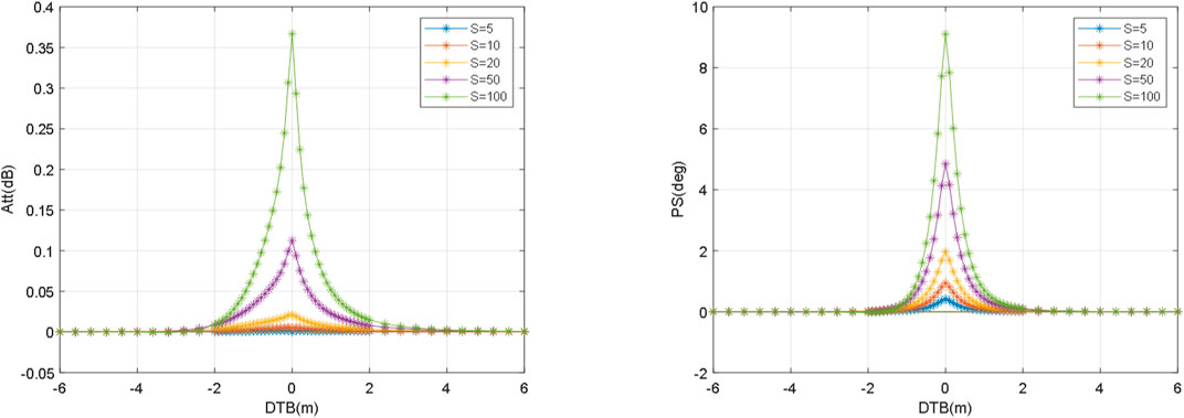
FIGURE 5. Response of the tilted receiver in different contrast stratum models.
The absolute values of the measured responses of VX and VR of the orthogonal receiving antenna are shown in Figure 6. VX and VR are the maximum values at the interface. These values show positive and negative alternate wave attenuation when the tool is far away from the interface. The absolute value is selected when drawing in the exponential coordinate system. This wave attenuation phenomenon may lead to multiple solutions during inversion. Therefore, orthogonal measurement antennas are often used in combination with axial conventional measurement antennas to obtain abundant formation information regarding conditions for inversion processing. The following analysis only considers the first node of fluctuation on both sides of the interface, that is, the first positive value. When the tool approaches the low-resistance layer from the high-resistance layer, the VR curve can predict the existence of the interface when it is 8–12 m and 2–7 m from the interface. Additionally, the edge detection distance of VX increases as the contrast ratio increases.
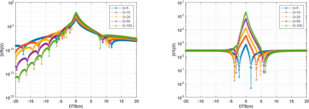
FIGURE 6. Response of the orthogonal receiver in different contrast stratum models.
It is worth noting that both the axial and tilted antenna measure the relative signal, that is, the ratio of two signals, which can reduce the systematic error of the tool. The orthogonal antenna measures the absolute signal and so anti-noise interference measures should be taken.
The stratum model 5 in Table 1 is selected and demonstrates the same spacing (1 m) between the transmitter and receiver and frequencies of 10 kHz, 50 kHz, 100 kHz, 500 kHz, and 2 MHz. The effects of different frequencies on the boundary detection characteristics of three antenna structures are also investigated.
The measured response of EATT and
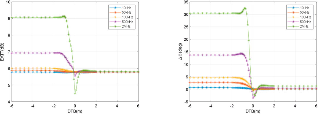
FIGURE 7. Response of the axial receiver at different frequencies.
The measured responses of ATT and PS of the tilted receiving antenna are shown in Figure 8. The figure reveals that the ATT and PS curves at five frequencies almost coincide and approach 0 when the tool is far from the interface. When the tool is close to the interface, ATT and PS gradually increase and reach the maximum value at the interface, which also rises with the increase in frequency. The oscillation occurs at the high-frequency interface of 2 MHz. At high frequencies, ATT and PS can predict the presence of the interface at 2 m near the interface. Meanwhile, at low frequency (10 kHz), ATT is less than 0.02 dB and cannot accurately measure the interface. Overall, the edge detection capability of PS is better than ATT.
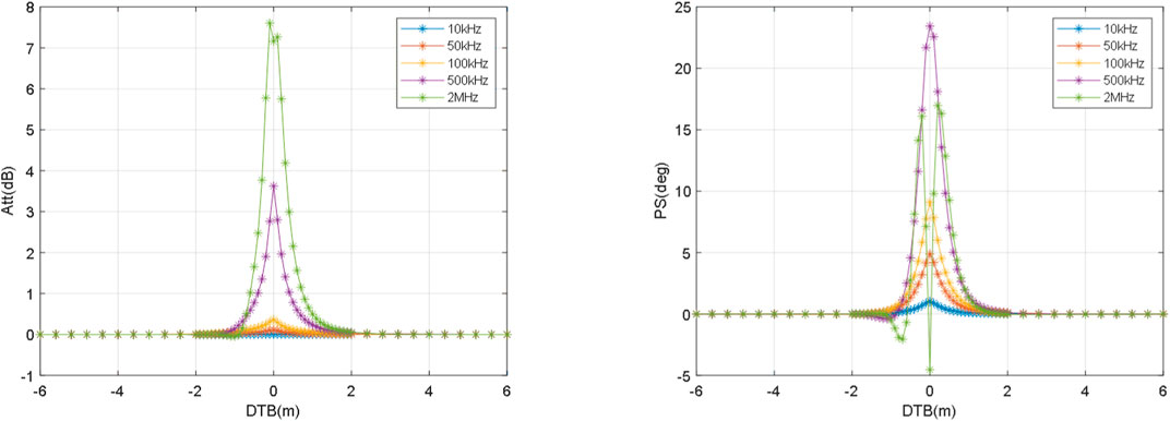
FIGURE 8. Response of the tilted receiver at different frequencies.
VX and VR have maximum values at the interface and increase with frequency, which is shown in Figure 9. High frequency induces rapid voltage attenuation, especially in the low-resistance layer. If the signal acquisition capacity is at 10 nV, then edge detection distances of VR at 10 kHz and 50 kHz are considerable when approaching the interface from the high-resistance layer. In this case, the presence of the interface can be predicted when it is 10 m from the interface. The edge detection distances of the VX curve at 50, 100, and 500 kHz are superior, and the interface is predicted to exist at 6 m near the interface.
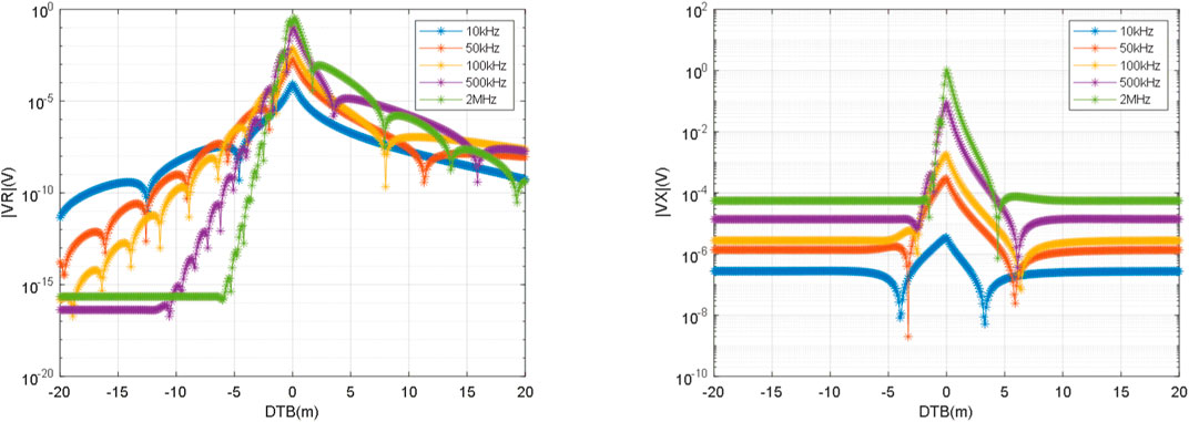
FIGURE 9. Response of the orthogonal receiver at different frequencies.
The stratum model 5 in Table 1 is selected, and the transmission frequency is set to 100 kHz. The spacing between the transmitter and receiver is the source distance at 1, 2, 4, and 6 m. The influence of different source distances on the boundary detection characteristics of three antenna structures was also investigated.
The response of the axial receiving antenna is affected by the spacing between the transmitting and receiving antennas and between the two receiving antennas. The spacing between the two receiving antennas is 8 in, and the measured response is shown in Figure 10. The figure reveals that the values of EATT and
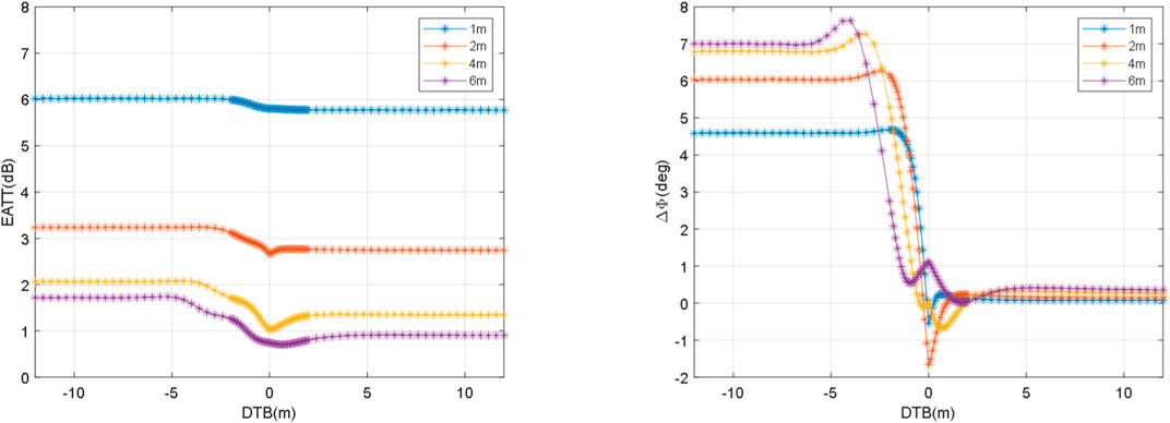
FIGURE 10. Response of the axial receiver at different source distances.
The source distance is 1 m, and the spacing between the two receiving antennas is 4, 6, 8, 10, and 12 in. The measured response of EATT and
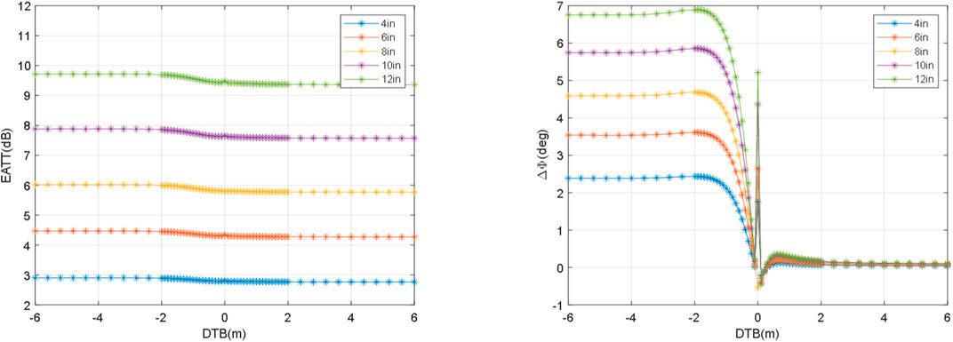
FIGURE 11. Response of the axial receiver at different spacings between the two receiving antennas.
The measurement responses of ATT and PS of the tilted receiving antenna are shown in Figure 12. The ATT and PS curves of the four frequencies nearly coincide and approach 0 when far away from the interface. When approaching the interface, ATT and PS with a short source distance gradually increase and reach the maximum at the interface, while ATT and PS with long source distance oscillate at the interface. When approaching the interface from high impedance, ATT and PS with a source distance of 6 m can predict the existence of the interface at 9 and 7 m away. Overall, the probe distance increases with the source distance.
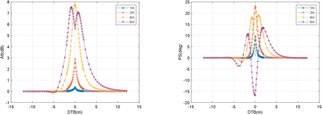
FIGURE 12. Response of the tilted receiver at different source distances.
The measured responses of VX and VR of the orthogonal receiving antenna reach a maximum at the interface and decrease with an increase in the source distance as shown in Figure 13. The source distance has a considerable influence on VX. When the tool approaches the low-resistance layer from the high-resistance layer, VX with a source distance of 6 m can predict the existence of the interface when it is 20 m away. Generally, a large source distance indicates a large probe distance.
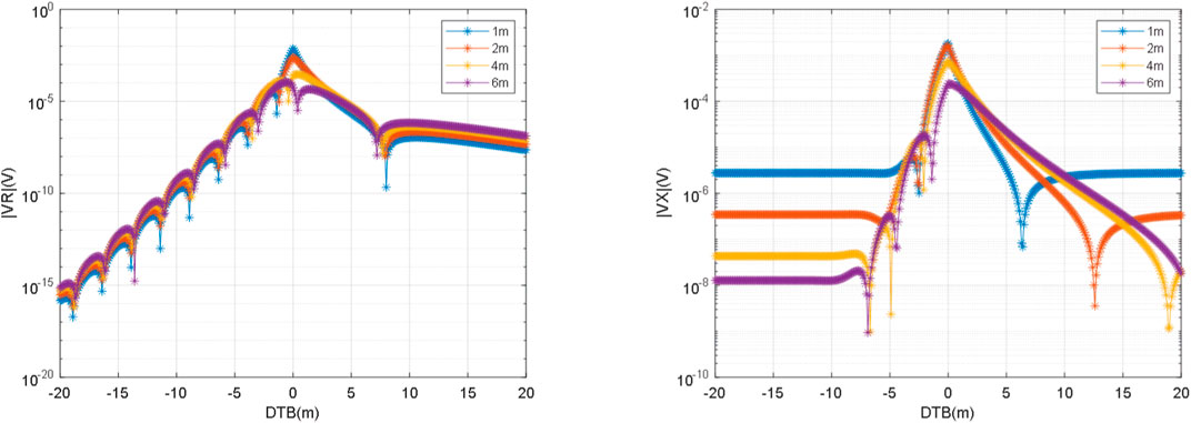
FIGURE 13. Response of the orthogonal receiver at different source distances.
Regarding resistivity measurements, the signals measured by axial transmitting and axial receiving antennas can effectively quantify the formation resistivity, while tilted and orthogonal receiving antennas can only measure the boundary information and cannot quantify the formation resistivity. Thus, combining an axial receiver with a tilted or orthogonal receiver is superior in the design of the electromagnetic boundary detection LWD tool. In this way, the formation resistivity can be quantified and the boundary information can be simultaneously measured.
For the application of formation, the axial antenna is only applicable to detecting the interface when approaching from a low-resistance layer, while the tilted and orthogonal receiving antennas demonstrate improved performance both in detecting the interface when approaching from high-resistance layers and low-resistance layers. The tilted antenna and orthogonal antenna complement the axial antenna in geological adaptability.
In terms of the factors that influence the capability of boundary detection, a decrease in frequency reduces the measured value, which is not conducive to the identification boundary of axial and tilted antennas. However, a decrease in frequency slows down the signal attenuation speed, which is conducive to the expansion of the edge detection range of the orthogonal antenna. The detection range of the three antenna systems is expanded with an increase in the spacing between the transmitter and receiver. However, the spacing between two axial receivers does not improve the expansion of the edge detection range. To obtain a larger detection depth, it is necessary to reduce the frequency to below 100 kHz and increase the spacing between the transmitter and receiver as much as possible.
The raw data supporting the conclusions of this article will be made available by the authors without undue reservation.
YT contributed to the conception and design of the study. JZ and YD supplemented the data analysis and modified the manuscript. All authors contributed to the revision of the manuscript, and read and approved the submitted version.
This research is supported by the 14th 5-Year Key Technology Program of CNPC (2021ZG04). The calculation was completed with the equipment of China National Logging Corporation.
The authors thank Dr. John Zhou of Maxwell Dynamics, Inc., for his professional and valuable help.
Authors YT, JZ, YD, LL, CY, and XW are employed by China National Logging Corporation. Authors YT, JZ, YD and CY were employed by Key Laboratory of Logging of China National Petroleum Corporation.
The remaining author declares that the research was conducted in the absence of any commercial or financial relationships that could be construed as a potential conflict of interest.
All claims expressed in this article are solely those of the authors and do not necessarily represent those of their affiliated organizations, or those of the publisher, the editors, and the reviewers. Any product that may be evaluated in this article, or claim that may be made by its manufacturer, is not guaranteed or endorsed by the publisher.
Anderson, W. L. (1979). Computer program: Numerical integration of related hankel transforms of orders 0 and 1 by adaptive digital filtering. Geophysics 44, 1287–1305. doi:10.1190/1.1441007
Antonsen, F., Olsen, P. A., Stalheim, S. O., Constable, M. V., Irondelle, M., Cook, M., et al. (2014). “Net pay optimization and improved reservoir mapping from ultra-deep look around LWD-measurements,” in Proceeding if the Abu Dhabi International Petroleum Exhibition and Conference, Abu Dhabi, UAE, November 2014. SPE-171856-MS. doi:10.2118/171856-MS
Bai, Y., Zhan, Q., Wang, H., Chen, T., He, Q., and Hong, D. (2020). Calculation of tilted coil voltage in cylindrically multilayered medium for well-logging applications. IEEE Access 8, 30081–30091. doi:10.1109/ACCESS.2020.2971535
Bell, C., Hampson, J., Eadsforth, P., Chemali, R., Helgesen, T., Meyer, H., et al. (2006). “Navigating and imaging in complex geology with azimuthal propagation resistivity while drilling,” in Proceeding if the SPE Annual Technical Conference and Exhibition, San Antonio, Texas, USA, September 2006. SPE-102637-MS. doi:10.2118/102637-MS
Bittar, M. S., Rodney, P. F., Mack, S. G., and Bartel, R. P. (1991). “A true multiple depth of investigation electromagnetic wave resistivity sensor: Theory, experiment, and prototype field test results,” in SPE annual technical conference and exhibition, proceedings. Paper 22705.
Chew, W. C. (1990). Waves and fifields in inhomogeneous media 1st ed. New York: Van Nostrand Reinhold Company, 133–147.
Clark, B., Luling, M. G., Jundt, J., Ross, M., and Best, D. (1988). “A dual depth resistivity measurement for FEWD,” in SPWLA annual logging symposium transactions. SPWLA-1988-A.
Clegg, N., Sinha, S., Rodriguez, K. R., Walmsely, A., Sviland-Østre, S., Lien, T., et al. (2022). “Ultra-deep 3D electromagnetic inversion for anisotropy, a guide to understanding complex fluid boundaries in a turbidite reservoir,” in Proceeding if the SPWLA 63rd Annual Logging Symposium, June 2022. SPWLA-2022-0119. doi:10.30632/SPWLA-2022-0119
Fan, Y., Hu, X., Deng, S., Yuan, X., and Li, H. (2019). Logging while drilling electromagnetic wave responses in inclined bedding formation. Petroleum Explor. Dev. 46 (4), 711–719. doi:10.1016/S1876-3804(19)60228-4
Fang, S., Merchant, A., Hart, E., and Kirkwood, A. (2008). “Determination of structural dip and azimuth from LWD azimuthal propagation resistivity measurements in anisotropic formations,” in Proceeding if the SPE Annual Technical Conference and Exhibition, Denver, Colorado, USA, September 2008. SPE-116123-MS. doi:10.2118/116123-MS
Hawkins, D., Phettongkam, N., and Nakchamnan, N. (2015). “Optimizing well placement in geosteering using an azimuthal resistivity tool in complex thin bed reservoirs in the gulf of Thailand,” in Proceeding if the SPWLA 56th Annual Logging Symposium, Long Beach, California, USA, July 2015. SPWLA-2015-FFFF.
Hu, X., Fan, Y., Deng, S., Yuan, X., and Li, H. (2020). Electromagnetic logging response in multilayered formation with arbitrary uniaxially electrical anisotropy. IEEE Trans. Geosci. Remote Sens. 58 (3), 2071–2083. doi:10.1109/TGRS.2019.2952952
Li, H., and Wang, H. (2016). Investigation of eccentricity effects and depth of investigation of azimuthal resistivity LWD tools using 3D finite difference method. J. Petroleum Sci. Eng. 143, 211–225. doi:10.1016/j.petrol.2016.02.032
Li, Q., Omeragic, D., Chou, L., Yang, L., Duong, K., Smits, J., et al. (2005). “New directional electromagnetic tool for proactive geosteering and accurate formation evaluation while drilling,” in Proceeding if the SPWLA 46nd Annual Logging Symposium, New Orleans, Louisiana, June 2005. SPWLA-2005-UU.
Li, K., Gao, J., Ju, X. D., Zhu, J., Xiong, Y. C., and Liu, S. (2018). Study on ultra-deep azimuthal electromagnetic resistivity LWD tool by influence quantification on azimuthal depth of investigation and real signal. Pure Appl. Geophys. 175 (12), 4465–4482. doi:10.1007/s00024-018-1899-5
Li, H., Zhu, J., Xiong, Y., Liu, G., Tian, Y., Geng, Z., et al. (2020a). On the depth of detection of logging-while-drilling resistivity measurements for looking-around and looking-ahead applications. Interpretation 8 (3), SL151–SL158. doi:10.1190/INT-2019-0291.1
Li, K., Gao, J., and Zhao, X. (2020b). Tool design of look-ahead electromagnetic resistivity LWD for boundary identification in anisotropic formation. J. Petroleum Sci. Eng. 184, 106537. doi:10.1016/j.petrol.2019.106537
Moran, J. H., and Gianzero, S. (1979). Effects of formation anisotropy on resistivity-logging measurements. Geophysics 44, 1266–1286. doi:10.1190/1.1441006
Nemushchenko, D., Zaputlyaeva, A., Sviridov, M., and Kuvaev, I. (2022). “Vendor-independent stochastic inversion models of azimuthal resistivity lwd data, case studies from the Norwegian continental shelf,” in Proceeding if the SPWLA 63rd Annual Logging Symposium, June 2022. SPWLA-2022-0111. doi:10.30632/SPWLA-2022-0111
Nikitenko, M., Itskovich, G. B., and Seryakov, A. (2020). Fast electromagnetic modeling in cylindrically layered media excited by eccentred magnetic dipole. Radio Sci. 51, 573–588. doi:10.1002/2016rs005950
Omeragic, D., Habashy, T., Esmersoy, C., Li, Q., Seydoux, J., Smits, J., et al. (2006). “Real-time interpretation of formation structure from directional EM measurements,” in Proceeding if the SPWLA 47th Annual Logging Symposium, Veracruz, Mexico, June 2006. SPWLA-2006-SSS.
Rabinovich, M., Le, F., Lofts, J., and Martakov, S. (2011). “Deep? How deep and what? The vagaries and myths of "look around" deep-resistivity measurements while drilling,” in Proceeding if the SPWLA 52nd Annual Logging Symposium, Colorado Springs, Colorado, May 2011. SPWLA-2011-NNN.
Rodney, P. F., Wisler, M. M., Thompson, L. W., and Meador, R. A. (1983). “The electromagnetic wave resistivity MWD tool,” in SPE annual technical conference and exhibition proceedings. SPE-12167-PA.
Seydoux, J., Legendre, E., Mirto, E., Dupuis, C., Denichou, J., Bennett, N., et al. (2014). “Full 3D deep directional resistivity measurements optimize well placement and provide reservoir scale imaging while drilling,” in Proceeding if the SPWLA 55th Annual Logging Symposium, Abu Dhabi, United Arab Emirates, May 2014. SPWLA-2014-LLLL.
Wang, T., Chemali, R., Hart, E., and Cairns, P. (2007). “Real-time formation imaging, dip, and azimuth while drilling from compensated deep directional resistivity,” in Proceeding if the SPWLA 48th Annual Logging Symposium, Austin, Texas, June 2007. SPWLA-2007-NNN.
Wang, L., Liu, Y., Wang, C., Fan, Y., and Wu, Z. (2021). Real-time forward modeling and inversion of logging-while-drilling electromagnetic measurements in horizontal wells. Petroleum Explor. Dev. 48 (1), 159–168. doi:10.1016/S1876-3804(21)60012-5
Wu, A., Fu, Q., Mwachaka, S. M., and He, X. (2019). Numerical modeling of electromagnetic wave logging while drilling in deviated well. J. Ambient. Intell. Humaniz. Comput. 10 (5), 1799–1809. doi:10.1007/s12652-018-0700-z
Wu, Z., Li, H., Han, Y., Zhang, R., Zhao, J., and Lai, Q. (2022). Effects of formation structure on directional electromagnetic logging while drilling measurements. J. Pet. Sci. Eng. 211, 110118. doi:10.1016/j.petrol.2022.110118
Zhou, J., Li, H., Rabinovich, M., and D'Arcy, B. (2016). “Interpretation of azimuthal propagation resistivity measurements: Modeling, inversion, application and discussion,” in Proceeding if the SPWLA 57th Annual Logging Symposium, Reykjavik, Iceland, June 2016. SPWLA-2016-HHHH.
Zhu, J., Die, Y., Tian, Y., and Zhou, J. (2021). “Deciphering the capabilities of look-ahead methods in LWD,” in Proceeding if the SPWLA 62nd Annual Logging Symposium, Virtual Event, May 2021. SPWLA-2022-0080. SPWLA-2021-0024. doi:10.30632/SPWLA-2021-0024
Keywords: azimuthal electromagnetic LWD, ultra-deep electromagnetic LWD, boundary detection, anisotropy resistivity, tilted antenna, orthogonal antenna
Citation: Tian Y, Zhu J, Die Y, Liu L, Yue C, Wang X and Zhu Y (2023) Boundary detection capability and influencing factors of electromagnetic resistivity while using drilling tools in a horizontal well. Front. Earth Sci. 10:1042353. doi: 10.3389/feart.2022.1042353
Received: 12 September 2022; Accepted: 23 November 2022;
Published: 25 January 2023.
Edited by:
Jingjing Guo, Southwest Petroleum University, ChinaReviewed by:
Maryam Khosravi, Isfahan University of Technology, IranCopyright © 2023 Tian, Zhu, Die, Liu, Yue, Wang and Zhu. This is an open-access article distributed under the terms of the Creative Commons Attribution License (CC BY). The use, distribution or reproduction in other forums is permitted, provided the original author(s) and the copyright owner(s) are credited and that the original publication in this journal is cited, in accordance with accepted academic practice. No use, distribution or reproduction is permitted which does not comply with these terms.
*Correspondence: Jun Zhu, emh1anVuX2NwbEBjbnBjLmNvbS5jbg==
Disclaimer: All claims expressed in this article are solely those of the authors and do not necessarily represent those of their affiliated organizations, or those of the publisher, the editors and the reviewers. Any product that may be evaluated in this article or claim that may be made by its manufacturer is not guaranteed or endorsed by the publisher.
Research integrity at Frontiers
Learn more about the work of our research integrity team to safeguard the quality of each article we publish.