Digital construction of geophysical well logging curves using the LSTM deep-learning network

A complete well logging suite is needed frequently, but it is either unavailable or has missing parts. The mudstone section is prone to wellbore collapse, which often causes distortion in well logs. In many cases, well logging curves are never measured, yet are needed for petrophysical or other analyses. Re-logging is expensive and difficult to achieve, while manual construction of the missing well logging curves is costly and low in accuracy. The rapid technical evolution of deep-learning algorithms makes it possible to realize the digital construction of missing well logging curves with high precision in an automated fashion. In this article, a workflow is proposed for the digital construction of well logging curves based on the long short-term memory (LSTM) network. The LSTM network is chosen because it has the advantage of avoiding the vanishing gradient problem that exists in traditional recurrent neural networks (RNNs). Additionally, it can process sequential data. When it is used in the construction of missing well logging curves, it not only considers the relationship between each logging curve but also the influence of the data from a previous depth on data at the following depth. This influence is validated by exercises constructing acoustic, neutron porosity, and resistivity logging curves using the LSTM network, which effectively achieves high-precision construction of these missing curves. These exercises show that the LSTM network is highly superior to the RNN in the digital construction of well logging curves, in terms of accuracy, efficiency, and reliability.

Introduction

During well logging operations, borehole damage or collapse occurs frequently in the mudstone section, resulting in distortion in well logs, and even more seriously, in missing well logging curves. Instrument failure and logging environments can also lead to lost or erroneous logging curves. In petrophysical analysis, a comprehensive analysis of all the depths of the well logging curves is usually a must. As a result, the distortion or absence of a particular section of the logging curve will have profound reverse effects on the results of the final analysis. Therefore, it is necessary for the entire logging curve to be reliable with high accuracy, for which an efficient, simple, and accurate logging curve construction method is particularly essential.

Re-logging can be used to obtain the missing logging curves. However, doing so will significantly increase the cost from the standpoint of both labor and equipment. Moreover, re-logged curves may deviate from those in the original logging environment due to changes in that environment, for example, mud-filtrate invasion. Many other methods for reconstructing the missing logging curves have been investigated in the literature, such as empirical formulas, correlation correction methods, forward modeling correction methods, and multi-variate regression methods (Zhang et al., 2018; Zhou et al., 2021). If the borehole collapses and the logging curve distortion is serious, the correlation correction method will not succeed. The forward modeling correction method requires accurate knowledge of the complex physical properties (Asquith et al., 2004; Bateman, 2012), which are not readily available. Although those methods can reconstruct the missing logging curve to a certain extent, they ignore the complexity and strong non-uniformity of the formation conditions, thus greatly simplifying the real formation conditions, and hindering the predicted results from meeting the accuracy requirements of logging interpretation and reservoir characterization (Bassiouni, 1994).

With the advancement of computer and information technology, machine learning has become a powerful tool for model construction and prediction (Ramaswamy et al., 2000; Cawley 2006; Kusiak et al., 2010; Marvuglia and Messineo, 2012; Hu et al., 2014), and has undoubtedly found applications in the field of petroleum exploration and production (Iturrar N-Viveros and Parra, 2014; Zerrouki et al., 2014; Chen 2020). Potential machine-learning algorithms include support vector machines (SVMs), artificial neural networks (ANNs), recurrent neural networks (RNNs), and generative adversarial networks (GANs) (Goodfellow et al., 2014; Goodfellow, 2016). Rolon et al. (2009) used the generalized regression neural network to reconstruct the missing logging curves, and the experimental results show that synthetic logging curves from the neural network are more accurate than those from traditional multi-variate regression, linear regression, and other methods (Rolon et al., 2009). Salehi et al. (2017) reconstructed density and electrical logs using the multilayer perceptron (MLP). Yang et al. (2008) used the back propagation (BP) neural network to reconstruct acoustic logging curves, and verified that the method could significantly improve the quality of acoustic logging curves affected by wellbore collapse. Hu (2020) adopted the GAN with constraint conditions to learn the distribution of real logging curves, and introduced the mean square error into the objective function of the original GAN to improve the learning ability of the model. He demonstrated that, compared with the Kriging interpolation method and the fully connected neural network, this method performs better in predicting the logging curve. However, although the above methods are able to reconstruct the missing well logging curves to a certain extent, it is still difficult to achieve high accuracy.

In this article, we demonstrate that the LSTM network is a deep-learning algorithm naturally suited to the digital reconstruction of well logging curves. This is because the well logging curve has the characteristic of a time sequence, due to the connection of the curve from point to point. When dealing with these kinds of data, we should not only consider the interaction between each well logging curve, but also the influence of the previous data point on the following data point. Recurrent neural networks (RNNs) are very effective in processing data with sequential characteristics (Schuster and Paliwal, 1997). However, a regular RNN has the problem of a vanishing gradient, which effectively prevents the weight in the neural network from changing its value and hence stops the neural network from further training.

The long short-term memory (LSTM) network (Hochreiter and Schmidhuber, 1997) is a variant of the RNN. Compared with the RNN, the LSTM network has three more control devices: input control, forget control, and output control, which can better retain the required data. The LSTM network overcomes the problem of the vanishing gradient that exists in the RNN, making it more effective and reliable for training the well logging curves. It has found application in many different domains. Zhao et al. (2021) developed a hybrid model by combining a long short-term memory network (LSTM), a convolutional neural network (CNN), and a singular spectrum analysis (SSA). Among these, the LSTM network effectively extracted the time features, and the hybrid model could accurately extract data features of monitoring signals and further improve the recognition performance of mass spectral signals. Thus, the long short-term memory network has significant advantages in processing time-series data. Shashidhar et al. (2022) adopted the LSTM method for visual speech recognition, and the research results show that this network can recognize speech very well. Ma et al. (2022) applied LSTM to predicting the normal passenger flow and emergency passenger flow of a metro traffic system. Compared with the traditional data of incoming and outgoing warehouse or IC cards, this method better reflects the passenger flow data of the metro traffic system’s capacity. Absar et al. (2022) used the LSTM model to predict infectious diseases, and their study showed that the algorithm achieved good results in time-series prediction, and could hence effectively reduce infection rates to a certain extent.

In this study, the LSTM method is used to reconstruct the missing logging curves through the TensorFlow (Martín et al., 2016) framework, and the reliability of the model is verified using field well logs. Experimental studies show that, compared to the RNN, the LSTM network is very efficient, accurate, and concise for the generation of digital well logging curves.

Methodology

Correlation analysis

Correlation analysis refers to the analysis of the degree of correlation between two or more variables. In this work, it is necessary to perform correlation analysis and find the logging curves that have the highest correlation with the target logging curve. The existence of some correlation is necessary to predict one variable from another. Pearson’s (1920) correlation coefficient is used to in this work. Assuming that there are two variables, X and Y, Pearson’s correlation coefficient between X and Y can be expressed as follows:

$\rho \left(X,Y\right)=\frac{cov\left(X,Y\right)}{{\sigma }_X{\sigma }_Y}=\frac{E\left(\left(X-{\mu }_X\right)\left(Y-{\mu }_Y\right)\right)}{{\sigma }_X{\sigma }_Y}=\frac{E\left(XY\right)-E\left(X\right)E\left(Y\right)}{\sqrt{E\left(X^2\right)-E^2\left(X\right)}\sqrt{E\left(Y^2\right)-E^2\left(Y\right)}},(1)$

where E represents the mathematical expectation and cov(X, Y) represents the covariance between variable X and variable Y; ${\mu }_X$ , ${\mu }_y$ are the mean for variable X and variable Y, respectively; and ${\sigma }_X,{\sigma }_Y$ are the standard deviation for variable X and variable Y, respectively. The value range of Pearson’s coefficient p is [-1,1]. The positive and negative values of the p-value represent the direction of correlation, and the magnitude of its absolute value represents the degree of correlation. When the p-value is greater than 0, X and Y are positively correlated, and the greater the p-value, the higher the correlation. By contrast, if the p-value is less than 0, X and Y are negatively correlated; if the p-value is 0, there is no linear relationship between X and Y; and if the absolute value of p is 1, X and Y are completely linearly correlated. A rule of thumb for measuring the significance of the correlation is as follows: 0.0 < | p | < 0.2 means very weakly related or unrelated, 0.2 < | p | < 0.4 means a weak correlation, 0.4 < | p | < 0.6 means moderately related, 0.6 < | p | < 0.8 means a strong correlation, and 0.8 < | p | < 1.0 means a very strong correlation.

Data normalization

The purpose of data normalization is to map large data or small data in a data set to the same range. The most common range is (0, 1), which is convenient for subsequent data processing and model training. The maximum and minimum normalization is adopted in this study, and its formula is shown as follows:

$x^{\prime }=\frac{x-x_{\mathit{min}}}{x_{\mathit{max}}-x_{\mathit{min}}},(2)$

where x is the data sample and x_max and x_min are the maximum and minimum values in the x sample, respectively. Using Eq. 2, all the data samples can be mapped to between 0 and 1.

The recurrent neural network

The recurrent neural network (Chung et al., 2015) is a kind of recursive neural network that takes sequence data as input, and recurses in the evolutionary direction of sequence where all nodes (cyclic units) are linked by chain. The RNN is very effective for processing sequential data, which are arranged in a certain chronological or logical order. The RNN simply consists of an input layer, a hidden layer, and an output layer, which is shown below.

Figure 1 is the basic structure of an RNN. It does not show all the nodes of the recurrent neural network. Assuming that the arrow above W is removed, this network becomes the most common fully connected neural network. The X vector represents the input layer data, S represents the value of the hidden layer, and the O vector represents the value of the output layer. It should be noted that in actual problems, the input layer, output layer, and hidden layer are not one node as shown in the figure above; instead, each layer actually contains multiple nodes. Here U is the weight from the input layer to the hidden layer, V is the weight from the hidden layer to the output layer, and W is the weight of the last hidden layer as the input for this time. It can therefore be seen that the hidden layer of the recurrent neural network is composed of the current input value X and the last hidden value S. An expanded recurrent neural network is shown below. The related formulas are as follows:

$O_t=g\left(V•S_t\right)(3)$

$S_t=f\left(U•X_t+W•S_{t-1}\right)(4)$

FIGURE 1

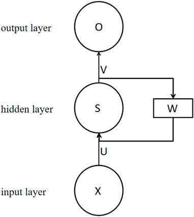
FIGURE 1. Basic structure of the recurrent neural network.

Figure 2 is the expansion of Figure 1. It can be seen from Figure 2 or Eq. 4 that the received value at time t in this network consists of the input X_t and the output of a hidden layer at a previous time, which reveals how the recurrent neural network works. It can be seen from Eqs 3, 4 that the specific calculation process of the recurrent neural network is obtained by multiplying the input by the corresponding weight before finally adding the activation function. Throughout the training process, the same weight W is used for each moment. A cyclic neural network is similar to a multilayer neural network: as the number of neurons increases, the RNN also has the problems of gradient explosion and gradient disappearance in the process of back propagation (Franke et al., 2012).

FIGURE 2

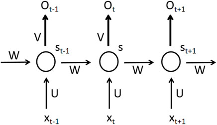
FIGURE 2. Expanded structure of the recurrent neural network.

The LSTM network

In order to eliminate the problems of gradient explosion, gradient disappearance etc., various improved recurrent neural networks have been proposed instead of the traditional RNNs. The long short-term memory network is a variant of the recurrent neural network. The recurrent neural network will store all the values of the hidden layer at each moment and apply them to the next moment, thus ensuring that each moment contains the information of the previous moment. The LSTM network selectively stores information by adding three gating devices, namely input control, output control, and forget control, compared with the hidden layer that stores all data in the recurrent neural network. The LSTM is composed of a series of recursively connected sub-networks of memory blocks, each of which contains one or more memory cells and three multiplication units (input gate, output gate, and forget gate), which can carry out continuous write, read, and reset operations on memory cells (Hochreiter and Schmidhuber, 1997; Graves et al., 2013). The LSTM can thus effectively mitigate the problems of gradient disappearance and gradient explosion that exist in the traditional RNN (Cho et al., 2014). The internal structure of the LSTM network is shown in Figure 3. Excluding the nodes in each neural unit, an LSTM network is an RNN.

FIGURE 3

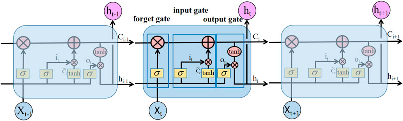
FIGURE 3. Structure of the LSTM network.

Firstly, the forget gate determines how much information in the unit state C_t-1 of the previous moment will be retained in the current moment C_t. The input X_t of the current moment is combined with the hidden state of the previous moment to form a new vector, and is then multiplied by the weight coefficient W, and finally through the sigmoid function. The result is multiplied by the unit state C_t-1 at the last moment to determine how much information is added to the unit state C_t-1 at the last moment. The expression of the forget gate control for this time is

$f_t=\sigma \left(W_f•\left[{\mathrm{h}}_{t-1},{\mathrm{X}}_t\right]+b_f\right)(5)$

Secondly, the input gate controls how much information from the input X_t of the current moment will be retained in the cell state C_t of the current moment. The sigmoid function determines which values need to be updated for the input gate layer. The tanh function determines the candidate value ${\stackrel{\sim }{C}}_t$ at the current time and is multiplied by the current i_t vector to finally determine how much of the candidate information is input into the cell state C_t, where the expression is

$i_t=\sigma \left(W_i•\left[{\mathrm{h}}_{t-1},{\mathrm{X}}_t\right]+b_i\right)(6)$

${\stackrel{\sim }{C}}_t=\mathit{tan}h\left(W_c•\left[{\mathrm{h}}_{t-1},{\mathrm{X}}_t\right]+b_c\right)(7)$

Finally, the output gate controls how much state C of the unit is output to the hidden state of the unit. The output gate and output signal are multiplied to determine the amount of information to be output at this moment. The expressions for decision vector O_t and the hidden state h_t of the cell unit are as follows:

$O_t=\sigma \left(W_o•\left[{\mathrm{h}}_{t-1},{\mathrm{X}}_t\right]+b_o\right)(8)$

$h_t=o_t*\mathit{tan}h\left(C_t\right)(9)$

The cell state exists in the whole process, and its function is to update the cell state, that is, to update C_t-1 to C, multiply the old state by f_t, discard unwanted information, add new candidate values, and determine the change of each cell state according to the result. The formula is as follows:

$C_t=f_t•C_{t-1}+i_t{\stackrel{\sim }{C}}_t(10)$

In the above expressions, X_t is the input data of the long short-term memory network at time t; h_t is the data output at time t; i_t, O_t, and f_t are the activation vector values of input gate, output gate, and forget gate of the LSTM neural network at time t of a node; W_f, W_i, W_c, and W_o are the corresponding weights of each structure, respectively; and b_i, b_c, and b_o are the offsets corresponding to each structure, respectively. C is the state of neuron cells, $\sigma$ is sigmoid function, and tanh is a hyperbolic tangent function.

Comparison of LSTM and RNN

Table 1 lists the comparison of the LSTM network and the RNN. The main advantage of the LSTM network is that it solves the problems of disappearing gradients in RNN, and is more suitable for processing long-memory time-series data.

TABLE 1

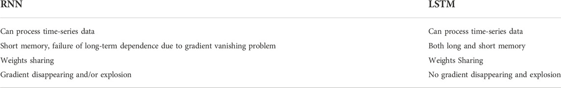
TABLE 1. Comparison of LSTM and RNN.

The optimization algorithms

Optimization algorithms are required in the model to update training and output parameters so that they approach or reach the optimum, thereby maximizing (or minimizing) the loss function (Kingma and Ba, 2015). Optimization algorithms are divided into three categories (Qing, 1999). The first category is gradient descent, which includes batch gradient descent, random gradient descent, and small batch gradient descent. These optimization algorithms optimize the model by minimizing the loss function. The second category is momentum optimization methods, including the momentum gradient descent method and the Nesterov accelerated gradient method (NAG). The last category is the adaptive learning rate optimization algorithm, including the AdaGrad, RMSProp, Adam, and AdaDelta methods (Kingma and Ba, 2015). Of these, the Adam (adaptive momentum) optimization algorithm is adopted in this study. This method can calculate the adaptive learning rate for each parameter. The flow chart for the Adam algorithm is shown in Figure 4.

FIGURE 4

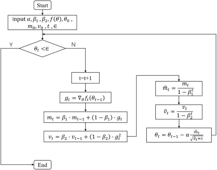
FIGURE 4. Flow chart for the Adam optimization algorithm.

In Figure 4, a is the learning rate, ß₁, ß₂ ⊂ [0,1) are to control the moving average index attenuation rate; f(θ) is the objective function; θ₀ is the vector for the initial parameter; m₀ is the initial first moment for the gradient (expectation); m₁ is the initial second moment for the gradient (expectation of the square of the gradient); ${\widehat{m}}_t$ and ${\widehat{v}}_t$ are the bias-corrected estimates; t is the time step; and e is a small number. We need to determine the objective function f(θ) and α, β₁, and β₂. Here a is generally 0.001, β₁ is 0.9, β₂ is 0.999, and e is 10⁻⁸. Meanwhile, we need to initialize the parameter vectors θ₀, the first-order moment vector m_t, the second-order moment vector v_t, and the time step t. Then we need to determine whether the current θ_t converges to less than e. If not, we update each part iteratively; that is, we update t to t+1, the gradient of parameter θ_t, the first order matrix m_t, and the second-order matrix v_t. Then we calculate the first order matrix estimation and the second-order matrix estimation. Finally, we update the parameter θ_t. Once the last θ_t value is less than ε, the iteration ends and the optimal θ_t value is found.

The Adam algorithm is different from the traditional stochastic gradient descent algorithm, which uses a single learning rate to update the weight, and the learning rate does not change in the training process. The Adam algorithm iteratively updates neural network weights based on training data. The Adam algorithm designs different adaptive learning rates for different parameters by calculating the first-order and second-order moment estimation of the gradient, which is the combination of two stochastic gradient descent methods. The adaptive gradient algorithm (AdaGrad) preserves a learning rate for each parameter to improve the performance of sparse gradients in natural language processing and computer vision. Root mean square propagation (RMSProp) adaptively preserves the learning rate for each parameter based on the mean of the nearest magnitude of the weight gradient, which means that the algorithm has good performance on unsteady and on-line problems. The Adam algorithm combines the advantages of the above two algorithms (Qing, 1999). It has the advantages of efficient computation, small memory consumption, and invariable gradient diagonal scaling. It is suitable for solving large-scale optimization problems with big data and parameters, as well as problems of high noise or sparse gradient, and has the advantage of an intuitive interpretation of hyperparameters.

Regularization

Regularization is a general term for a class of methods that add extra terms to loss functions in machine learning to prevent overfitting and to improve model performance. Common regularizations are ${\mathit{l}}_1$ regularization and ${\mathit{l}}_2$ regularization, or ${\mathit{l}}_1$ norm and ${\mathit{l}}_2$ norm. The model using ${\mathit{l}}_1$ regularization is called lasso regression, and the model using ${\mathit{l}}_2$ regularization is called ridge regression. The linear regression ${\mathit{l}}_1$ regularization loss function is

$\underset{w}{\mathit{min}}\left[{\displaystyle \sum }_{i=1}^N{\left(w^T{x}_i-y_i\right)}^2+\lambda {\Vert w\Vert }_1\right](11)$

while the ${\mathit{l}}_2$ regularization loss function is

$\underset{w}{\mathit{min}}\left[{\displaystyle \sum }_{i=1}^N{\left(w^T{x}_i-y_i\right)}^2+\lambda {\Vert w\Vert }_2^2\right](12)$

In Eqs 11, 12, ω represents the coefficient of a feature, and the regularization term puts a limit on the coefficient. Here ${\mathit{l}}_1$ is regularized as the sum of the absolute values of the elements in the weight vector w, and ${\mathit{l}}_2$ is regularized as the sum of squares of the elements in the weight vector w. The regularization term is preceded by a coefficient λ, whose value determines the relative importance of the two terms in Eq. 12. In order to prevent overfitting in this work, ${\mathit{l}}_2$ regularization is used to constrain weight and bias.

Experiments and results analysis

The field well logs used in this study are from X field, including 13 logging curves, namely, computed gamma ray (CGR), uranium (URAN), potassium (POTA), thorium (THOR), shallow lateral resistivity (LLS), deep lateral resistivity (LLD), spontaneous potential (SP), natural gamma ray (GR), borehole diameter (CALI), photoelectric factor (PEF), neutron porosity (NPHI), density (RHOB), and sonic interval transit time (DTCO). There are two natural gamma ray logs: CGR and GR, of which GR is from conventional GR logging, while CGR is from GR spectrometry logging. CGR is the computed gamma ray, subtracting uranium from total gamma ray is the summation of thorium and potassium sources (Doveton, 1994). As a result, GR is larger than CGR. Four groups of experiments are conducted: Exercise 1 assumes that there are missing data in the upper section of the sonic log curve (DTCO). Exercise 2 assumes that there are missing data in the lower section of the sonic log curve (DTCO). Exercise 3 assumes that there are missing data in the neutron porosity logging curve (NPHI), and Exercise 4 assumes a portion of the LLD curve is missing. Results from the linear and logarithmic domain are then compared. From there, we perform analysis on the results and provide an overall evaluation. For all the exercises, and for comparison purposes, we plot the results from both LSTM and RNN side-by-side.

Data and model preparation

The following steps are taken to prepare the data and model.

Step 1: Correlation analysis

Pearson correlation coefficients are computed for the original well-logging curves to check the correlation between all the curves and to help select the training data with strong correlations with the target well-logging curve. We emphasize that the Pearson correlation coefficient only checks the linear relationship between the curves. However, the curves may have some degree of nonlinear relationships. In this work, the Pearson correlation coefficient is used to provide the first degrees of correlation between the curves. In other words, it serves as a reference. The final feature selection also incorporates human experience. In fact, because not many features are involved, using the Pearson correlation coefficient with human judgement is in general sufficient for well logs; the advanced feature selection method is not required.

Step 2: Data normalization

All the original well-logging curves are properly normalized using equation 2 given in Section 2.2 and mapped to between 0 and 1. Here we emphasize that for the resistivity logs, the normalization, training, and digital construction are performed in the logarithm domain.

Step 3: Data transformation

The normalized data are transformed into supervised data to a common input format for training time-series models such as the LSTM network or RNN.

Step 4: Data training

The above processed data are divided into training set, validation set, and test set, which comprise 60%, 20%, and 20% of the data, respectively. The training set is used to adjust the deep learning network parameters to minimize the loss function. By studying the training loss with the epoch and the validation loss with the epoch, we can see if the model is overfitting. If the result is not desired, the model structure and hyperparameters, such as the learning rate, the number of trainings, and batch size should be adjusted accordingly.

The performance of the model is optimized by comparing the training loss with the validation loss. Figure 5 shows part of the network optimization process: The model in Figure 5A shows that the validation loss is higher than the training loss at one time, and the other way around at another time, which indicates the model is unstable. In this case, the number of trainings and batch processing samples need to be increased. Generally speaking, with an increase in the number of trainings, the number of weight updates in the network will also increase, which is beneficial for model fitting. The larger the number of batch samples, the more will be sampled from the original data set each time, and the easier it will be to ensure that the distribution of batch samples is similar to that of the original data set. Figure 5B shows that it is difficult for the training loss and the validation loss to coincide after the inflection point, which may indicate that the network converges very slowly due to the low learning rate, and so it is necessary to increase the learning rate. If the learning rate is increased to 0.01, for example, as shown in Figure 5C, a sawtooth appears as the epoch increases, and the loss value hovers around the optimal value. It is possible that the learning rate is too large and that it directly skipped the lowest value. It is therefore necessary to appropriately reduce the learning rate to 0.001. For example, in Figure 5D, the training loss and verification loss appear to coincide at the end, indicating that a model with a better performance has been trained and achieved.

FIGURE 5

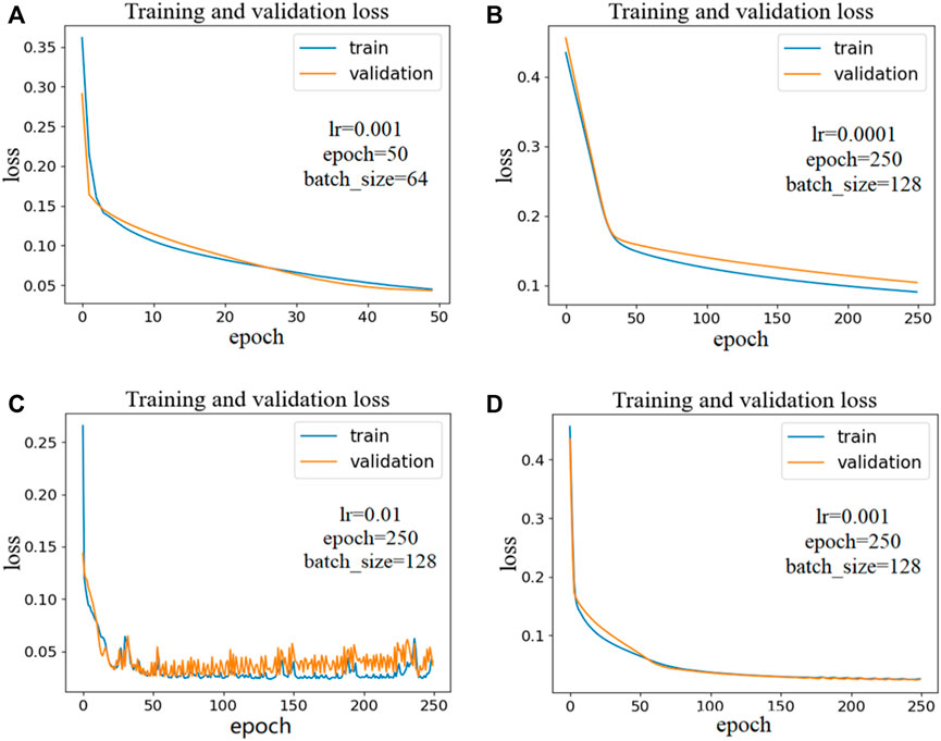
FIGURE 5. Model optimization. (A) Unstable case; (B) Learning rate too small; (C) Learning rate too large; (D) Optimal case.

Experiments

The experimental environment is Tensor flow 2.5.0 with Python 3.9. The parameters of the LSTM network model constructed in this article are as follows: There is one LSTM network layer; there are 50 neurons in each hidden layer; and there is 1 neuron in the output layer. The weight and bias in the loss function are added into the ${\mathit{l}}_2$ regularization term, and the regularization coefficients are all set to 0.01. The loss function adopts mean absolute error (MAE) and the optimization algorithm adopts Adam. The model is trained in 250 epochs and 128 models are processed in batches each epoch. Part of the well logs (about 20%) are manually removed to simulate the missing logs.

Exercise 1 (upper acoustic curve missing)

Assuming the sonic logging curve between the depth of 12,699.0 ft and 12,909.5 ft is missing, we first compute the Pearson correlation matrix of the curves, which is show in Figure 6.

FIGURE 6

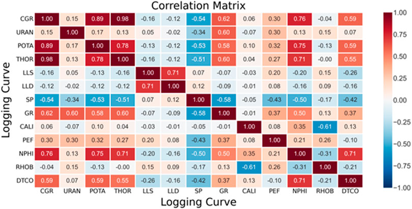
FIGURE 6. Pearson correlation matrix for all the logging curves.

It can be seen from Figure 6 that CGR, POTA, THOR, GR, and NPHI have relatively high positive correlation with DTCO, while SP has the highest negative correlation with DTCO. Note that we select the logging curves with the highest correlation with DTCO, although this does not necessarily mean the correlation is actually strong. For example, the correlation between CGR and DTCO is 0.59, which is moderately correlated at best. In this experiment, six logs—CGR, POTA, THOR, GR, NPHI, and SP—are selected to train the LSTM network and the RNN, and are then used to reconstruct the missing part of the sonic logging curve. The training data in the model consists of two complete logging sections, from a depth of 12,450.0 ft to a depth of 12,699.0 ft and from a depth of 12,909.5 ft to a depth of 13,500.0 ft. The logging interval is 0.5 ft. The reconstructed sonic logging curve using the LSTM model and the RNN model are shown in the last two panels of Figure 7.

FIGURE 7

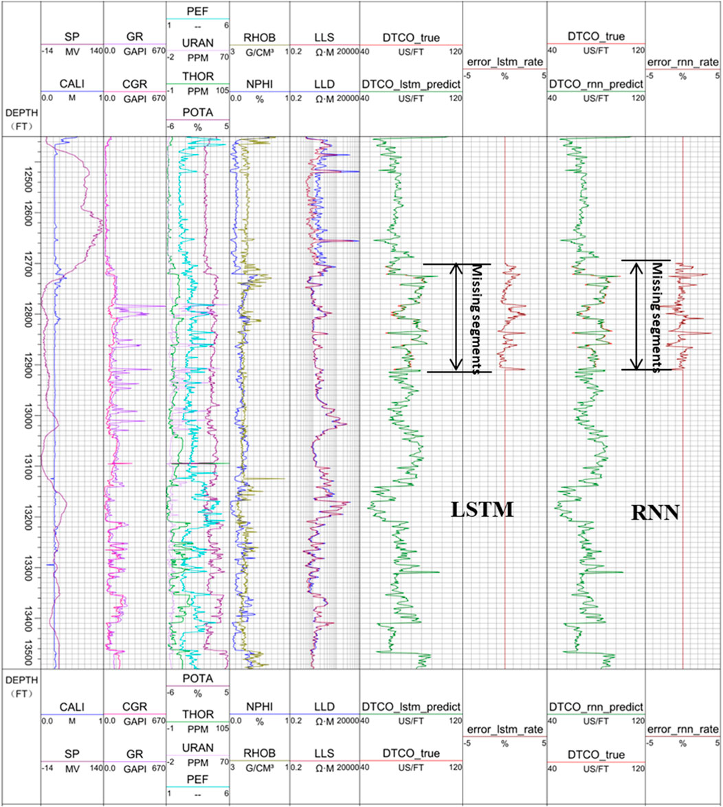
FIGURE 7. Reconstructed sonic logging curve between the depth of 12,699.0 ft and 12,909.5 ft.

In Figure 7, panel 6 and panel 7 show the comparison between the original sonic logging curve (red) and the reconstructed sonic logging curve using the LSTM (green, barely seen, because it is so close to the original curve), and the prediction error in percentage, while panel 8 and panel 9 show the comparison of the original sonic logging curve (red) and the reconstructed sonic logging curve using the RNN (green, barely seen, because it is so close to the original curve), and the prediction error in percentage. Clearly, both reconstructed sonic logging curves match the original curve very well, with the maximum error within 2%. However, the errors from the LSTM are much smaller than those from the RNN.

Exercise 2 (lower acoustic curve missing)

In this exercise, we construct the lower section of the sonic logging curve, between 12,949.0 ft and 13,159.5 ft. Figure 8 shows the reconstructed sonic logging curves.

FIGURE 8

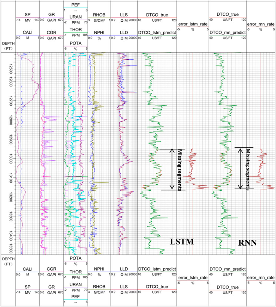
FIGURE 8. Reconstructed sonic logging curve between 12,949.0 ft and 13,159.5 ft.

Similar to Figure 7, in Figure 8, panel 6 and panel 7 show the comparison of the original sonic logging curve (red) and the reconstructed sonic logging curve using the LSTM (green, barely seen, because it is so close to the original curve), and the prediction error in percentage, while panel 8 and panel 9 show the comparison of the original sonic logging curve (red) and the reconstructed sonic logging curve using the RNN (green, barely seen, because it is so close to the original curve), and the prediction error in percentage. Clearly, both reconstructed sonic logging curves match the original curve well, with the maximum error within 5%. The errors (including pattern and magnitude) from the LSTM are similar to those from the RNN. The reason for the reconstruction at different sections on the same logging curve is to avoid contingency, which demonstrates that using the LSTM network to reconstruct well logging curves has universal applicability.

Exercise 3 (partial absence of neutron porosity logging curve)

In practice, acoustic, neutron porosity, density, and other logging curves may be missing. In order to verify that the LSTM network is capable of reconstructing logging curves other than the sonic logging curve, we assume in this case that the neutron porosity logging curve section between 12,949.0 ft and from a depth of 13,159.5 ft is missing. It can be seen from the correlation matrix in Figure 5 that CGR, POTA, THOR, GR, and DTCO have positive correlation with NPHI, while SP has a negative correlation with NPHI. In this experiment, six logs: CGR, POTA, THOR, GR, DTCO, and SP are used to train the LSTM network, and then to reconstruct the neutron porosity curve. The training data in the model consists of two complete logging sections, from a depth of 12,450.0 ft to a depth of 12,949.0 ft, and from a depth of 13,160 ft to a depth of 13,500.0 ft. The logging interval is 0.5 ft. The reconstructed neutron porosity logging curves using the LSTM and RNN models are shown in Figure 9.

FIGURE 9

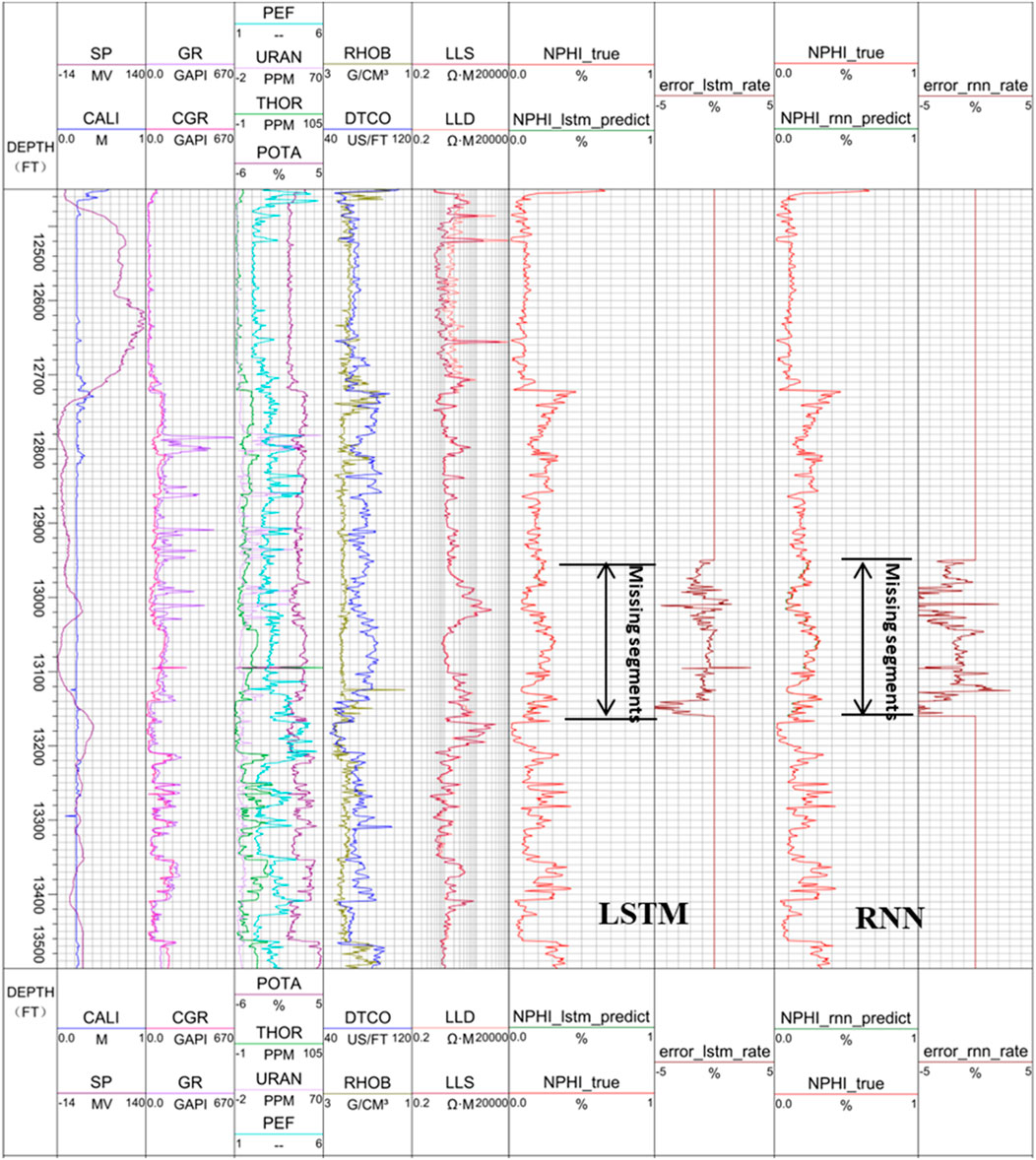
FIGURE 9. Reconstructed neutron porosity logging curve between 12,949.0 ft and 13,159.5 ft.

In Figure 9, panel 6 and panel 7 show the comparison between the original NPHI logging curve (red) and the reconstructed NPHI logging curve using the LSTM (green, barely seen, because it is so close to the original curve), and the prediction error in percentage, while panel 8 and panel 9 show the comparison of the original NPHI logging curve (red) and the reconstructed NPHI logging curve using the RNN (green, barely seen, because it is so close to the original curve), and the prediction error in percentage. Clearly, both reconstructed sonic logging curves match the original curve very well, with the maximum error within 5%. However, the errors from the LSTM are much smaller than those from the RNN. The peak error at the depth of around 13090 ft is apparently caused by the peak in POTA and CGR. As a result, more data cleaning is needed before the prediction.

Exercise 4 (portion of deep lateral logging curve is missing)

For Exercises 1-3, the predicted curve, either the sonic logging curve or neutron porosity curve, belongs to porosity-related curves, both having nice correlations with lithology-related logging curves, such as GR or SP. The digital construction of those curves is rather stable with high accuracy. In this exercise, we predict the deep resistivity logging curve (LLD), which is related to another petrophysical parameter, fluid saturation, to see how the LSTM network performs. To do so, we select the LLS curve, NPHI curve, and DTCO curve for the model training. For the resistivity curve, we compare the performance between the linear domain and the logarithmic domain. The predicted LLD curves in the linear resistivity domain using both the LSTM and RNN for the missing segment are shown in Figure 10, while those in the logarithmic resistivity domain are shown in Figure 11.

FIGURE 10

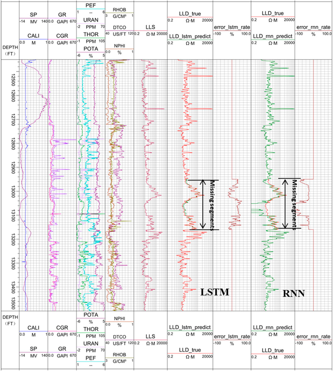
FIGURE 10. Reconstructed LLD logging curve between 12,949.0 ft and 13,159.5 ft in linear resistivity domain.

FIGURE 11

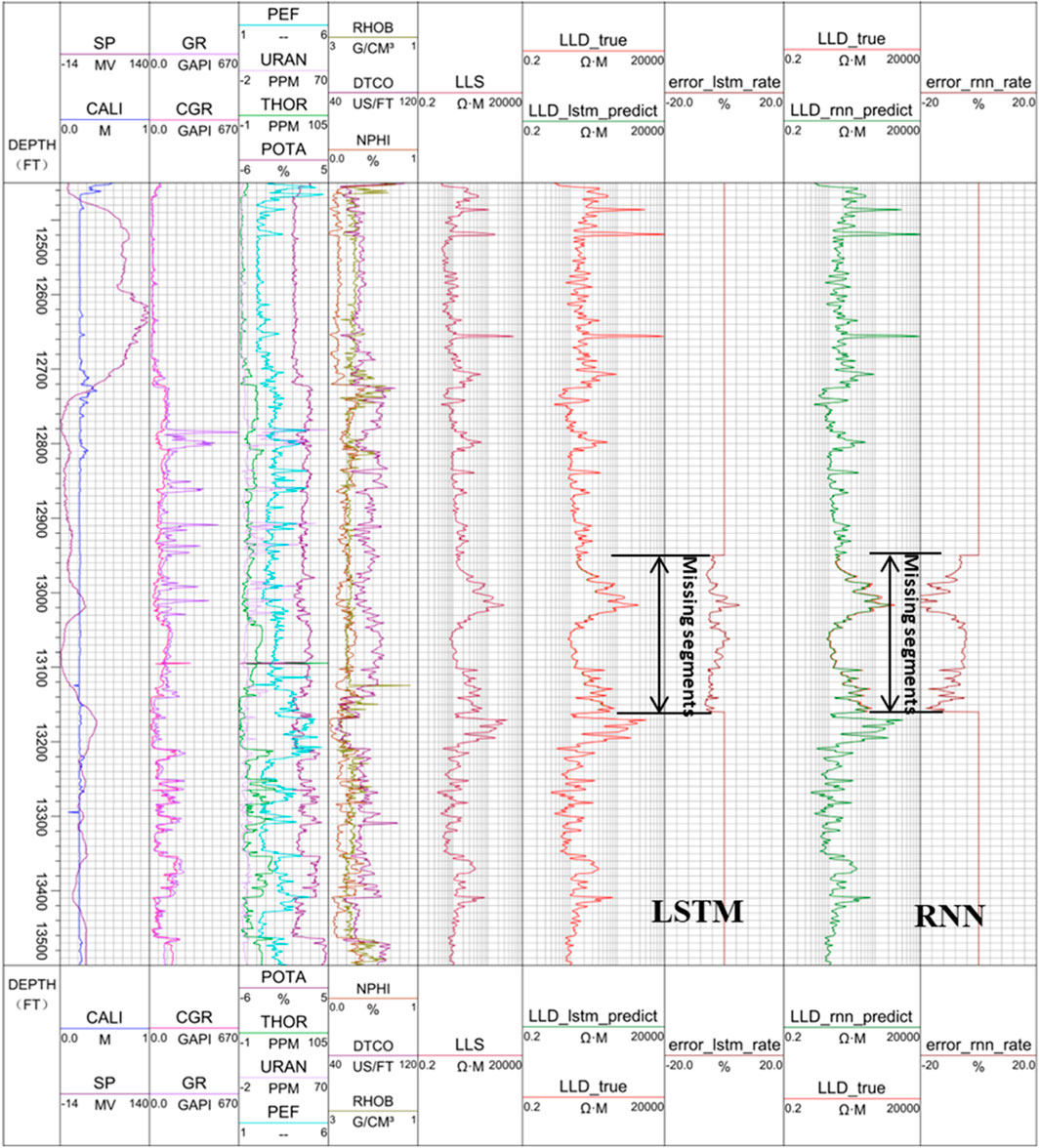
FIGURE 11. Reconstructed LLD logging curve between 12,949.0 ft and 13,159.5 ft in logarithmic resistivity domain.

From panel 6 and panel 7 of Figure 10 and Figure 11, we can see that the reconstructed LLD curve from the LSTM is very close to the original LLD curve, especially in the logarithmic resistivity domain. The result in the logarithmic resistivity domain is much better than that in the linear domain. In the logarithmic domain, the error is within 5%, while in the linear domain, some of the error can be as high as 20%. From panel 8 and panel 9 of Figure 10 and Figure 11, we can see that the reconstructed LLD curve from the RNN is much worse than that from the LSTM, with some of the error as high as 100% in the linear resistivity domain, and 20% in the logarithmic domain.

Results analysis

It can be seen from Figures 7–11 that by using the LSTM network one can reconstruct the missing sonic, neutron porosity, and deep resistivity logging curves with very high accuracy using the dataset in this study, and the results are much more accurate than those from the RNN. We expect the procedure has universal applicability. Table 2 shows the comparison of the LSTM and RNN parameters for Exercise 1, 2, and 4. Clearly the RMSEs from the LSTM for the three cases are much smaller than those from the RNN, with only half the training time.

TABLE 2

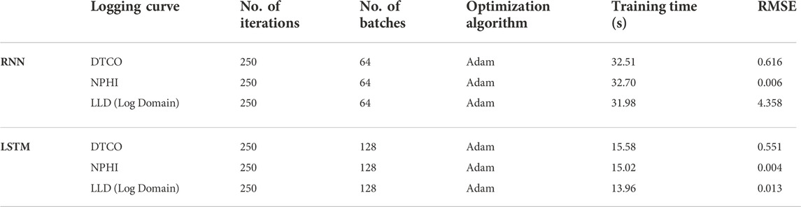
TABLE 2. The parameters for the LSTM and RNN.

Due to the special gate design of the LSTM, the network training not only takes into account the dependence of each log curve, but also the influence of the previous depth on the future depth. This enables the LSTM network to not only take full advantage of the nonlinear characteristics between logs, but also to learn the characteristics of the logs as they vary with the logging depth. In addition, compared with the RNN, the LSTM network has three more gating devices, so it can effectively solve the problems of gradient disappearance and gradient explosion present in the RNN. Moreover, the LSTM network has the capability of handling long-term memory to include effects of longer well-logging sequences. As a result, the LSTM network has shorter training time, and the results are much more accurate than those from the RNN. Digital logging curve construction can thus be effectively and efficiently performed using the LSTM network.

Conclusion

In this study, the LSTM network is used to reconstruct three types of logging curves with the following findings:

1) The network reconstructs all the missing sonic, neutron porosity, and deep resistivity logging curves very well.

2) The resistivity construction should be conducted in the logarithmic domain.

3) Comparative study shows that the results from the LSTM network are much more accurate than those from the traditional RNN.

As a special type of RNN, the LSTM network has an added three gating devices, which make it more useful for the reconstruction of logging curves due to its inherent memory characteristics and ability to handle gradient disappearance and/or explosion. The network allows for automatically finding the logging curves possessing strong correlations with the target curve to serve as a training set for the model, thereby saving the cost of manual data processing, and avoiding the limitations of traditional empirical formulas and statistical analysis reconstruction. In this study, 60% of the total logging segments are used as the training data for the LSTM network model, which achieves very accurate reconstructions with the advantages of cost saving, high accuracy, robustness, and intelligence. This finding could pave the way for digital construction of well logs using deep-learning algorithms in the future.

Data availability statement

The data analyzed in this study is subject to the following licenses/restrictions: Since the data used in the study are confidential, the authors do not have permission to share data. Requests to access these datasets should be directed to ggao@yangtzeu.edu.cn.

Author contributions

JL and GG: conceptualization, methodology; JL: programming and analysis, writing—original draft (Chinese); GG: supervision, resources, writing—review, editing, English translation. Both authors have read and agreed to the published version of the manuscript.

Conflict of interest

The authors declare that the research was conducted in the absence of any commercial or financial relationships that could be construed as a potential conflict of interest.

Publisher’s note

All claims expressed in this article are solely those of the authors and do not necessarily represent those of their affiliated organizations, or those of the publisher, the editors, and the reviewers. Any product that may be evaluated in this article, or claim that may be made by its manufacturer, is not guaranteed or endorsed by the publisher.

Abbreviations

AdaGrad, adaptive gradient algorithm; ANN, artificial neural network; BP, back propagation; CALI, borehole diameter; CGR, computed gamma ray; CNN, convolutional neural network; DTCO, sonic interval transit time; GAN, generative adversarial networks; GR, natural gamma ray; LLD, deep lateral resistivity; LSTM, Long short-term memory network; LLS, shallow lateral resistivity; MLP, multilayer perceptron; NPHI, neutron porosity; P, Pearson correlation coefficient; PEF, photoelectric factor; POTA, potassium; RHOB, density; RMSProp, root mean square propagation; RMSE, root mean square error; RNN, recurrent neural network; SSA, singular spectrum analysis; SP, spontaneous potential; SVM, support vector machine; THOR, thorium; URAN, uranium.

References

Absar, N., Uddin, N., Khandaker, M. U., and Ullah, H. (2022). The efficacy of deep learning-based LSTM model in forecasting the outbreak of contagious diseases. Infect. Dis. Model. 7 (1), 170–183. doi:10.1016/j.idm.2021.12.005

PubMed Abstract | CrossRef Full Text | Google Scholar

Asquith, G. B., Kpygowski, D., and Gibson, C. R. (2004). Basic well log analysis. Tulsa: American Association of Petroleum Geologists.

Google Scholar

Bassiouni, Z. (1994). Theory, measurement and interpretation of well logs. SPE Textb. 4, 384. doi:10.2118/9781555630560

CrossRef Full Text | Google Scholar

Bateman, R. M. (2012). Openhole log analysis and formation evaluation. 2nd ed. Richardson, Texas: Society of Petroleum Engineers.

Google Scholar

Cawley, G. C. (2006). “Leave-One-Out cross-validation based model selection criteria for weighted LSSVMs,” in the 2006 IEEE International Joint Conference on Neural Network Proceedings, 16-21 July 2007 (Vancouver, Canada: IEEE), 1661–1668.

CrossRef Full Text | Google Scholar

Chen, Y. (2020). “Study of well logging curve reconstruction based on Machine learning,” (Beijing: University of Beijing). Thesis.

Google Scholar

Cho, K., Merrienboer, B. V., Gulcehre, C., Ba Hdanau, D., Bougares, F., Schwenk, H., et al. (2014). Learning phrase representations using RNN encoder-decoder for statistical machine translation. Comput. Sci. 2014, 1724–1734. doi:10.3115/v1/D14-1179

CrossRef Full Text | Google Scholar

Chung, J., Culcehre, C., Cho, K., and Bengio, Y. (2015). Gated feedback recurrent neural networks. Comput. Sci. 37 (2), 2067–2075. doi:10.48550/arXiv.1502.02367

CrossRef Full Text | Google Scholar

Doveton, J. H. (1994). Geological log interpretation. Tulsa, Oklahoma, United States: Society for Sedimentary Geology.

Google Scholar

Franke, T., Buhler, F., and Cocron, P. (2012). Enhancing sustainability of electric vehicles: A field study approach to understanding user acceptance and behavior. Advances in traffic Psychology 1 (1), 295–306.

Google Scholar

Goodfellow, I. J., Pouget-Abadie, J., Mirza, M., Xu, B., WardeFarley, D., Ozair, S., et al. (2014). “Generative adversarial nets,” in Proceedings of the 27th International Conference on Neural Information Processing Systems, 08 October 2014 (Montreal, Canada: MIT Press), 2672–2680.

Google Scholar

Goodfellow, I. NIPS 2016 tutorial: Generative adversarial networks. arXiv preprint arXiv: 1701.00160, 2016.(Accessed December 31, 2016).

Google Scholar

Graves, A., Mohamed, A., and Hinton, G. (2013). “Speech recognition with deep recurrent neural networks,” in IEEE International Conference on Acoustics, Speech and Signal Processing, Vancouver, BC, Canada, 26-31 May 2013 (IEEE), 6645–6649.

CrossRef Full Text | Google Scholar

Hochreiter, S., and Schmidhuber, J. (1997). Long short-term memory. Neural Comput. 9 (8), 1735–1780. doi:10.1162/neco.1997.9.8.1735

PubMed Abstract | CrossRef Full Text | Google Scholar

Hu, C., Jain, G., Zhang, P., Schmidt, C., Gomadam, P., and Gorka, T. (2014). Data-driven method based on particle swarm optimization and k-nearest neighbor regression for estimating capacity of lithium-ion battery. Appl. Energy 129, 49–55. doi:10.1016/j.apenergy.2014.04.077

CrossRef Full Text | Google Scholar

Hu, J. Q. (2020). “Logging Curve Prediction and reservoir identification based on deep learning,” (Shaanxi: University of science and technology). Master’s Thesis.

Google Scholar

Iturrar N-Viveros, U., and Parra, J. O. (2014). Artificial Neural Networks applied to estimate permeability, porosity and intrinsic attenuation using seismic attributes and well-log data. J. Appl. Geophys. 107, 45–54. doi:10.1016/j.jappgeo.2014.05.010

CrossRef Full Text | Google Scholar

Kingma, D. P., and Ba, J. (2015). “Adam: A method for stochastic optimization,” in Proceedings of 3rd Conference for Learning Representations, 7-9 May 2015 (Ithaca, New York: arXiv), 1–15.

Google Scholar

Kusiak, A., Li, M., and Zhang, Z. (2010). A data-driven approach for steam load prediction in buildings. Appl. Energy 87 (3), 925–933. doi:10.1016/j.apenergy.2009.09.004

CrossRef Full Text | Google Scholar

Ma, J., Zeng, X., Xue, X., and Deng, R. (2022). Metro emergency passenger flow prediction on transfer learning and LSTM model. Appl. Sci. 12 (3), 1644. doi:10.3390/app12031644

CrossRef Full Text | Google Scholar

Martín, A., Barham, P., Chen, J., Chen, Z., and Zhang, X. (2016). TensorFlow: A system for large-scale machine learning. Berkeley, California, United States: USENIX Association.

Google Scholar

Marvuglia, A., and Messineo, A. (2012). Monitoring of wind farms’ power curves using machine learning techniques. Appl. Energy 98, 574–583. doi:10.1016/j.apenergy.2012.04.037

CrossRef Full Text | Google Scholar

Pearson, K. (1920). Notes on the history of correlation. Biometrika 13 (1), 25–45. doi:10.1093/biomet/13.1.25

CrossRef Full Text | Google Scholar

Qing, N. (1999). On the momentum term in gradient descent learning algorithms. Neural Netw. 12 (1), 145–151. doi:10.1016/s0893-6080(98)00116-6

PubMed Abstract | CrossRef Full Text | Google Scholar

Ramaswamy, S., Rastogi, R., and Shim, K. (2000). Efficient algorithms for mining outliers from large data sets. SIGMOD Rec. 29 (2), 427–438. doi:10.1145/335191.335437

CrossRef Full Text | Google Scholar

Rolon, L., Mohaghegh, S. D., Ameri, S., Gaskari, R., and McDaniel, B. (2009). Using artificial neural networks to generate synthetic well logs. J. Nat. Gas. Sci. Eng. 1 (4-5), 118–133. doi:10.1016/j.jngse.2009.08.003

CrossRef Full Text | Google Scholar

Salehi, M. M., Rahmati, M., Karimnezhad, M., and Omidvar, P. (2017). Estimation of the non-records logs from existing logs using artificial neural networks. Egypt. J. Petroleum 26 (4), 957–968. doi:10.1016/j.ejpe.2016.11.002

CrossRef Full Text | Google Scholar

Schuster, M., and Paliwal, K. K. (1997). Bidirectional recurrent neural networks. IEEE Trans. Signal Process. 45 (11), 2673–2681. doi:10.1109/78.650093

CrossRef Full Text | Google Scholar

Shashidhar, R., Patilkulkarni, S., and Puneeth, S. B. (2022). Combining audio and visual speech recognition using LSTM and deep convolutional neural network. Int. J. Inf. Technol. 22, 1–12. doi:10.1007/s41870-022-00907-y

CrossRef Full Text | Google Scholar

Yang, Z. L., Zhou, L., Peng, W. L., and Zheng, J. Y. (2008). Application of BP neural network technology in sonic log data rebuilding. J. Southwest Petroleum Univ. 2008 (01), 63–66. doi:10.3863/j.issn.1000-2634.2008.01.017

CrossRef Full Text | Google Scholar

Zerrouki, A., Aifa, T., and Baddari, K. (2014). Prediction of natural fracture porosity from well log data by means of fuzzy ranking and an artificial neural network in Hassi Messaoud oil field, Algeria. J. Petroleum Sci. Eng. 115, 78–89. doi:10.1016/j.petrol.2014.01.011

CrossRef Full Text | Google Scholar

Zhang, D., Chen, Y., and Jin, M. (2018). Synthetic well logs generation via recurrent neural networks. Petroleum Explor. Dev. 45 (04), 629–639. doi:10.1016/s1876-3804(18)30068-5

CrossRef Full Text | Google Scholar

Zhao, Y., Xu, H., Yang, T., Wang, S., and Sun, D. (2021). A hybrid recognition model of microseismic signals for underground mining based on CNN and LSTM networks. Geomatics, Nat. Hazards Risk 12 (1), 2803–2834. doi:10.1080/19475705.2021.1968043

CrossRef Full Text | Google Scholar

Zhou, X., Cao, J., Wang, X., Wang, J., and Liao, W. (2021). Data-driven S-wave velocity prediction method via a deep-learning-based deep convolutional gated recurrent unit fusion network. Prog. Geophys. 86, M185–M196. doi:10.1190/geo2020-0886.1

CrossRef Full Text | Google Scholar