Crustal velocity structure in the South Yellow Sea revealed by the joint tomographic inversion of reflected and refracted seismic waves

The crustal velocity structure in the South Yellow Sea (SYS) Basin is crucial for understanding the basin’s geological structure and evolution. OBS (ocean-bottom station) data from the OBS2013 line have been used to determine the crustal velocity structure in the SYS. The velocity model of the upper crust in the northern SYS was determined using first-arrival traveltime tomography. The model showed a higher resolution shallow crustal velocity structure but a lower resolution middle-lower crustal velocity structure. The crustal velocity structure, together with the Moho discontinuity in the SYS Basin, was also constructed using a human–computer interactive traveltime simulation, and the result was highly dependent on the prior knowledge of the operator. In this study, we reconstructed a crustal velocity model in the SYS Basin using a joint tomographic inversion of the traveltime and its gradient data of the reflected and refracted waves picked from the OBS data. The resolution of the inverted velocity structure from shallow-to-deep crust was improved. The results revealed that the massive high-velocity body below the Haiyang Sag of the Jiaolai Basin extends to the Qianliyan Uplift in the SYS; the low-velocity Cretaceous strata directly cover the pre-Sinitic metamorphic rock basement of the Sulu orogenic belt; and the thick Meso-Paleozoic marine strata are retained beneath the Meso–Cenozoic continental strata in the northern depression. The Moho depth in the SYS Basin ranges from 28 to 32 km.

Introduction

The South Yellow Sea (SYS) Basin, the main part of the Lower Yangtze region, is located in the continental shelf area between the Chinese Continent and the Korean Peninsula. With a total area of approximately 280,000 km² and a sea-bottom depth of less than 80 m, oil and gas exploration in the SYS Basin has never made a breakthrough. In 2013, the Qingdao Institute of Marine Geology of the China Geological Survey, in conjunction with the First Institute of Oceanography of the Ministry of Natural Resources and the Institute of Geology and Geophysics, Chinese Academy of Sciences, implemented the joint land–sea deep seismic exploration line OBS2013 (Figure 1, blue dotted line) (Liu et al., 2015) in the Jiaodong, Bohai, and SYS regions, which aimed to study the structure of oil- and gas-bearing basins accompanied by the morphology of Moho discontinuity and deep structures in the exploration area. With the OBS2013 line data, Zou et al. (2016) generated a velocity structure model of the upper crust in the northern part of the SYS using first-arrival traveltime tomography. Zhao et al. (2019a) obtained a continuous 2-D velocity and interface model by using a human–computer interaction simulation of refraction and reflection traveltime data picked from OBS2013. Zhang et al. (2021) processed and analyzed the converted shear wave of the OBS data by forward simulation of the shear wave data. Liu et al. (2021) constructed the crustal velocity structure in the SYS Basin by using a human–computer interaction simulation of the refraction and reflection traveltime picked from OBS data combined with gravity data and obtained the approximate shape of the Moho discontinuity. Among the aforementioned studies, the resolution of velocity in the shallow layer inverted using first-arrival traveltime tomography is high, but that in the middle-to-lower layer is low. The velocity structures and the Moho morphology obtained by employing the human–computer interaction simulation are heavily dependent on operator expertise.

FIGURE 1

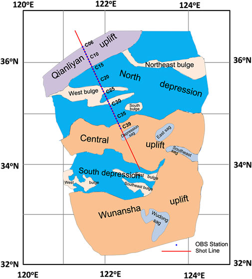
FIGURE 1. Tectonic regionalization of the SYS Basin and the position of survey line OBS2013.

To obtain a more precise velocity model and reduce the impact of human factors, this article proposes a joint tomographic inversion which can simultaneously use the traveltime and its gradient data of the reflected and refracted waves to invert the underground velocity model without determining the corresponding relationship between the seismic events and the reflection interfaces beforehand (Billette and Lambar, 1998). Moreover, the traveltime gradient can reflect the direction of ray propagation at the shot point and receiver point to solve the multipath problem of reflected rays, strengthen the constraint on the model space, and improve the inversion effect (Jin and Zhang, 2018). However, this requires picking the gradients in common-source gathers and in common-receiver ones, respectively. In data from survey line OBS2013, the OBS distance is large (6 km); in this case, the gradients cannot be picked in common-source gathers. To address this issue, we used a phase-shift wave-field extrapolation and the principle of reciprocity between a source and a receiver to pick the gradients in common-source gathers so that it becomes possible to use the joint tomography method (Alerini et al., 2009). Through this method, the crustal velocity structure and the undulating shape of the Moho discontinuity along this line are obtained. The related scientific problems are discussed, and some new understandings are attained.

Geological structure of the South Yellow Sea Basin and OBS2013 data

Tectonic division of the South Yellow Sea Basin

The SYS Basin is located to the east of the Tanlu Fault Zone and south of the Sulu Orogenic Belt. Its northern and southern edges are adjacent to the Sino-Korean block and South China block, with the Sulu Orogenic Belt and the Jiangshao Fault Belt as the boundaries, respectively. Moreover, the basin connects to the Lower Yangtze Subei Basin in the west. Overall, it is a superimposed basin on the Meso-Paleozoic marine strata which have been significantly transformed by Meso-Cenozoic tectonic plate movements (Wan, 2012; Li et al., 2017). The current SYS Basin is delimited in conformity with the stratigraphic distribution range since the Cretaceous–Paleogene extinction. From north to south, the basin can be categorized into five secondary structural units, namely, the Qianliyan Uplift, Northern depression, Central Uplift, Southern depression, and Wunansha Uplift (Figure 1). A series of faulted depressions, grabens, and other structures have also developed in the basin. The faulted depressions are primarily distributed to the west of 123°E and are characterized as northern faults in addition to the southern stratigraphic overlap, and the faulted depressions are steep in the north, and gentle in the south. Most of the structural lines are NNE and NE, controlling the basin’s formation and development. The Mesozoic strata in the Northern depression, together with the Paleozoic strata in the Central Uplift and the Wunansha Uplift, have feasible hydrocarbon potential. Moreover, the OBSs of the OBS2013 survey line are essentially arranged in the south of the Qianliyan Uplift and the whole Northern depression.

OBS2013 data

OBS2013 survey line, with a length of 223 km, is the first deep seismic survey line deployed in the SYS area. A total of 39 OBSs (C06–C39 in Figure 1) are deployed, including 17 short periodic MicroOBSs and 22 short periodic GeoprosOBSs. The distance between the OBSs is 6 km, and the sampling interval of the seismic wave is 4 ms. Additionally, the 2,501 shots are fired at a spacing of 125 m. The initial shot point is located at OBS03, and the termination shot point is 106 km away from OBS39 (red line in Figure 1).

It is necessary to note that we have denoised the OBS data to improve the signal-to-noise ratio (SNR). Due to the shallow-water depth and large wind waves in the area where the OBSs were located, a substantial amount of noise is found in the seismic records. Among the noise, random noise can be practically divided into low-frequency surge noise with a frequency of 0–3 Hz, high-frequency wind–wave noise with a frequency above 30 Hz, and ship-dynamic noise and coastal–industrial noise with a frequency of 20–200 Hz. Moreover, coherent noise can be generally classified into surface waves, shallow-reflection multiples, and water waves that are mainly concentrated in the direct-wave region, as well as wide-angle virtual reflection and deep refraction multiples positioned outside the direct-wave region (Zhao et al., 2020). According to the distribution characteristics of noise, data preprocessing comprises automatic gain control, bandpass filtering, and predictive deconvolution (Peacock and Treitel, 1969; Garret et al., 2012; Zhao et al., 2020).

Figure 2A illustrates the seismic phase identification of the post-noise reduction OBS19 seismic records (converted speed of 6 km/s), in which the Ps seismic phase is the inflected seismic phase in the sedimentary layer appearing on both sides of the station as the first arrival, and its apparent velocity is low. Pg1 is the refracted phase in the upper crust, followed by the Ps phase in the form of the first arrival. Simultaneously, the reflected seismic phase PsP at the bottom interface of the sedimentary layer can be identified near the converted traveltime of 1.5 s, exhibiting a significant hyperbolic symmetry. The Pb seismic phase of the left branch (the refraction seismic phase under the basement of the SYS’s continental basin) is reduced from 2 s to 1.2 s at the 20-km offset due to the Qianliyan Fault, and then the seismic phase can be continuously traced to the 90-km offset. The PcP seismic phase (the reflected wave seismic phase at the upper and lower crust interfaces) appears at 20–80 km, and the converted traveltime ranges from 1.5 s to 2.5 s. The PmP phase (Moho reflection phase) appears at an offset of 90 km and a traveltime of 3.5 s. The reflected seismic facies PcP in the high-velocity marine sedimentary layer are recorded at 20 km of the right branch and extend to approximately 45 km. The Pg2 seismic phase (refracted phase in the mid-crust) occurs at 45–65 km, and the equivalent traveltime ranges from 3 to 4 s. In addition, the PmP phase appears at 70–135 km, with weak phase energy. At 120 km, the Pn seismic phase (upper mantle refraction seismic phase) appears at the conversion time of 1 s with weak energy (Liu et al., 2021; Zhang et al., 2021).

FIGURE 2

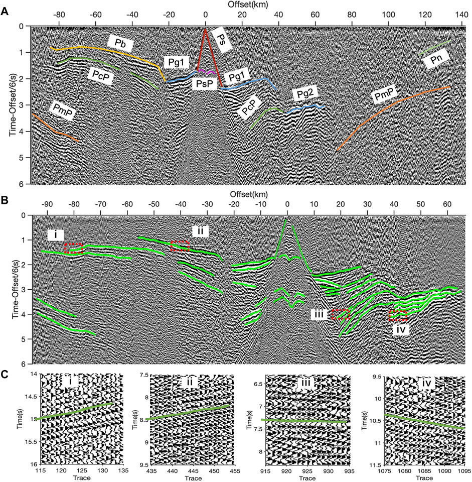
FIGURE 2. Seismic phase and event-picking of OBS19: (A) seismic phase identification of OBS19 seismic records, (B) seismic event-picking position of OBS19 seismic records, (C) the close-up of the pickup effect of the red dashed rectangles (i, ii, iii, and iv) in (B).

Methodology

For the tomographic inversion, the traveltimes and their gradients must be picked from the reflected and refracted phases in common-source and common-receiver gathers, respectively. Given the large OBS distance, we picked the traveltimes and their gradients of the same phase in the common-source gathers based on the principle of reciprocity. Since the sources are close to the sea surface and the OBS is located on the sea bottom, the sources are corrected to be located at the sea bottom by using a wave-field extrapolation technique to meet the principle of reciprocity.

Wave-field extrapolation

At present, the common wave equation datum correction methods can be divided into three categories: Kirchhoff integration method, finite difference method, and phase-shift method. The two previous methods are approximate solutions, while the wave equation transformed in the phase-shift will not distort the waveform and has high accuracy. Therefore, this study used the phase-shift method in the frequency–wavenumber domain to implement wave-field extrapolation (Gazdag, 1978; Cui et al., 2007; Alerini et al., 2009), redatuming and interpolation of the sources at receiver positions. First, the seismic records were transformed from the time–space domain to the frequency domain by using the Fourier transform. Afterward, wave-field extrapolation was performed using the “step-by-step accumulation” and “step-by-step parking” methods (Yang et al., 2007).

Picking traveltimes and their gradients at common-receiver gathers

The traveltime gradient refers to the tangent slope of the local correlation event in the seismic record at the center trace. It is the ratio of the traveltime difference △t between the two ends of the local coherent-phase axis centered on the track and the distance ∆x between them. Because the source spacing is small, the traveltime and its gradient at each source can be picked in the common-receiver gather by using the slant stack method (Schleicher, et al., 2008).

Picking traveltimes and their gradients at common-shot gathers

Since the number of OBSs was small and the interval was large, the number of seismic records in a common source was insignificant, making the tracking of seismic events even more challenging. The aforementioned slant-stacking method was unsuitable for picking the seismic event traveltimes and the gradient data at each receiver point in the common-source gather. This study applied the principle of reciprocity between a source and a receiver to the traveltime and gradient pickup of the sparse OBS observation system (Alerini et al., 2009). Figure 3 presents the details of its principle. For the seismic records T1 with the receiver at r₁ and the source at s₁, the traveltime gradient $p_1^s$ at source s₁ in the common-receiver gathers is picked, as exemplified in Figure 3A. As shown later, we circumvent the problem of picking slopes in common-source gathers by applying reciprocity of Green’s functions and using information from common-receiver gathers. Concerning the seismic records T2 with the receiver point at r₂ and the source at s₂, the traveltime gradient $p_2^s$ at point s₂ is picked in the common-receiver gathers, as illustrated in Figure 3B. In this way, we obtained the two gradients (Figure 3C).

FIGURE 3

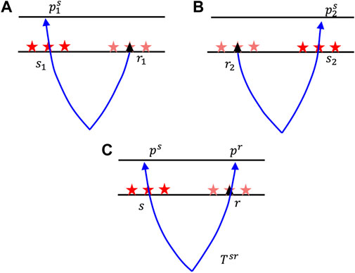
FIGURE 3. Schematic diagram of the principle of reciprocity: (A) Picking of data on common-receiver gathers at source s₁, (B) picking of data on common-receiver gathers at source s₂, and (C) use of the reciprocity to obtain the two gradients. The stars represent the sources and the triangles the receivers.

Joint tomographic inversion of reflected and first-arrival waves

The first arrival includes direct and refraction waves, and its event traveltime and gradient data are straightforward to pick. The first arrival of small and medium offsets can describe a shallow seabed’s characteristics, and the first arrival of large offsets can also reflect the deep strata information. In contrast, the observation angle of the reflected wave is limited, but the reflected wave contains a considerable amount of mid-deep information, which is more beneficial in the inversion of mid-deep crustal velocity. The joint tomographic inversion using first-arrival and reflected wave data can increase the coverage angle of the rays and their coverage times (Prieux et al., 2013; Liu and Zhang, 2022). Compared with a single first-arrival or reflected wave, joint inversion has a higher accuracy.

Following stereo-tomography (Billette et al., 2003; Lambare et al., 2004), the smooth velocity model was estimated from the traveltime and its gradient data of the local coherent events of both first-arrival and reflection waves. By modifying the velocity model and the location of the reflection points, the calculated and picked traveltimes and their gradients of the first-arrival and reflected waves are made consistent, thereby obtaining the underground velocity model (Li et al., 2019).

In joint tomography, the data space d of traveltime and its gradient tomography can be expressed as:

$\begin{array}{c}\mathrm{d}={\left[{\left({\mathrm{x}}_{\mathrm{s}},{\mathrm{z}}_{\mathrm{s}},{\mathrm{p}\mathrm{x}}_{\mathrm{s}},{\mathrm{x}}_{\mathrm{r}},{\mathrm{z}}_{\mathrm{r}},{\mathrm{p}\mathrm{x}}_{\mathrm{r}},{\mathrm{t}}_{\mathrm{s}\mathrm{r}}\right)}_{\mathrm{n}}\right]}_{\mathrm{n}=1}^{\mathrm{N}}\end{array},(1)$

where $\left({\mathrm{x}}_{\mathrm{s}},{\mathrm{z}}_{\mathrm{s}}\right)$ is the coordinate of the source s; $\left({\mathrm{x}}_{\mathrm{r}},{\mathrm{z}}_{\mathrm{r}}\right)$ is the coordinate of the receiver r; ${\mathrm{p}\mathrm{x}}_{\mathrm{s}}$ and ${\mathrm{p}\mathrm{x}}_{\mathrm{r}}$ are the traveltime gradients at the source and receiver points, respectively; and ${\mathrm{t}}_{\mathrm{s}\mathrm{r}}$ is the two-way traveltime. The subscript n represents the nth ray pair, and N represents the number of ray pairs.

The model space $\mathrm{m}$ is composed of discrete velocity parameters ${\mathrm{m}}_{\mathrm{v}}$, first-break wave section parameters ${\mathrm{m}}_{\mathrm{f}\mathrm{s}{\mathrm{t}}_{\mathrm{r}\mathrm{a}\mathrm{y}}}$, and reflection wave section parameters ${\mathrm{m}}_{{\mathrm{r}\mathrm{e}\mathrm{f}}_{\mathrm{r}\mathrm{a}\mathrm{y}}}$, which can be expressed as:

$\begin{array}{c}\mathrm{m}={\left({\mathrm{m}}_{\mathrm{v}},{\mathrm{m}}_{\mathrm{f}\mathrm{s}{\mathrm{t}}_{\mathrm{r}\mathrm{a}\mathrm{y}}},{\mathrm{m}}_{\mathrm{r}\mathrm{e}{\mathrm{f}}_{\mathrm{r}\mathrm{a}\mathrm{y}}}\right)}^{\mathrm{T}}\end{array}.(2)$

The objective function of joint tomographic inversion is:

$\begin{array}{c}\begin{array}{c}O\left(m_{fs{t}_{ray}},m_{re{f}_{ray}},m_v\right)=\frac{1}{2}\phi {\left[d_{fs{t}_{cal}}\left(m_{fs{t}_{ray}},m_v\right)-d_{fs{t}_{obs}}\right]}^T{C}_d^{-1}\left[d_{fs{t}_{cal}}\left(m_{fs{t}_{ray}},m_v\right)-d_{fs{t}_{obs}}\right]\\ +\frac{1}{2}\left(1-\phi \right){\left[d_{{ref}_{cal}}\left(m_{{ref}_{ray}},m_v\right)-d_{{ref}_{obs}}\right]}^T{C}_d^{-1}\left[d_{{ref}_{cal}}\left(m_{{ref}_{ray}},m_v\right)-d_{{ref}_{obs}}\right]\\ +\frac{1}{2}\lambda {\left(m_v-m_{v_{prior}}\right)}^T{C}_m^{-1}{L}^{T}L\left(m_v-m_{v_{prior}}\right),\end{array}\end{array}(3)$

where the first two items are the data residuals, and the third item is the model constraint. Additionally, $\phi$ is the first-arrival inversion weight; $\lambda$ is the damping coefficient that adjusts the relative size of the model constraint item role; $d_{fs{t}_{obs}}$ and $d_{fs{t}_{cal}}$ are the first-arrival observation data and calculation data, respectively; and $d_{{ref}_{obs}}$ and $d_{{ref}_{cal}}$ are the reflected-wave observation data and calculation data, respectively. $m_v$ is the model, $m_{v_{prior}}$ is the a priori model; $L$ represents the Laplace operator which carries on the smooth constraint to the model; $T$ superscript is the matrix transpose, and $C_d$ and $C_m$ are the covariance matrices of the data and the model, respectively. The data items and model parameter items are weighted, and the observation data with different magnitudes, such as the traveltime and gradient, and the model parameters with different magnitudes, such as the velocity and reflection point position, are normalized.$d_{cal}\left(m\right)$ is a nonlinear function. At the initial model $m_{v_{prior}}$, the function is expanded by using Taylor series, and the linear term is obtained:

$\begin{array}{c}{d}_{cal}\left(m\right)=d_{cal}\left(m_{v_{prior}}\right)+G\left(m-m_{v_{proor}}\right)\end{array},(4)$

where $G={\left(G_v,G_{ray}\right)}^T$, $G_v$ is the kernel function matrix of the data about the node velocity of the discrete model, and $G_{ray}$ is the kernel function matrix of the data about the ray parameters (reflection point coordinates, ray exit angle, and ray traveltime) (Billette and Lambar, 1998).

In order to obtain the minimum solution of objective function (3), after substituting Eq. 4 into Eq. 3, making the derivative of objective function model space parameter equal to 0, then the following linear inversion equation is obtained:

$\begin{array}{c}\left(\begin{array}{cc}{G}_v^T{C}_d^{-1}{G}_v& G_{ray}^T{C}_d^{-1}{G}_{ray}\\ \lambda C_m^{-1}L& 0\end{array}\right)\left(\begin{array}{c}∆m_v\\ ∆m_{ray}\end{array}\right)=\left(\begin{array}{c}{G}_v^T{C}_d^{-1}∆d\\ 0\end{array}\right),\end{array}(5)$

where $∆d$ represents the data residual vector, its element is the difference between the observed data and the data calculated by the current inversion model, and $∆m_v$ and $∆m_{ray}$ are the corrections of the ray segment parameters and discrete velocity values, respectively. In this way, it will continue iteratively until the mean square error between the inversion model calculation data and the observation data meets the given error limit.

Results

Picking traveltimes and their gradients

In total, 39 OBSs were encoded into the OBS2013 survey line in the SYS, of which 29 OBSs collected valid data. After preprocessing the robust OBS data, consistent with the OBS water-depth data, we extended the shot point from the sea surface to the seabed where the OBS was located using the phase-shifting wave-field extrapolation method from Chapter 3. Additionally, the local event traveltime and its gradient of the common source were picked through the principle of the reciprocity method. Figures 2B, C illustrate the result of the traveltimes and their gradients picked at the common receiver (OBS19). Then, Figure 2B portrays the pickup effect of the traveltime position at OBS19. The first-arrival seismic phases (Ps, Pb, Pg1, and Pg2) and reflected-wave seismic phases (PcP, PsP, and PmP) are picked. Moreover, Figure 2C displays the close-up of the picked effect of the red dashed rectangles (i, ii, iii, and iv). For all the valid OBS data, 284 groups of the first-arrival traveltimes and their gradients, along with 395 groups of reflection traveltimes and their gradients, were picked.

Joint tomographic inversion of traveltimes and their gradients

The crustal velocity distribution is inverted by the tomography using 284 groups of first-arrival traveltimes and their gradients, as well as 395 groups of reflection traveltimes and their gradients. According to the previous information on surface velocity in the study area and the velocity model constructed by the predecessors, the initial velocity model in Figure 4A is established. The model’s length in the x direction is 200 km, the depth in the z direction is 40 km, the velocity increases linearly with depth, v= (2 + 0.2z) km/s, and the size of the initial discrete unit of the model is 4 km × 1.5 km.

FIGURE 4

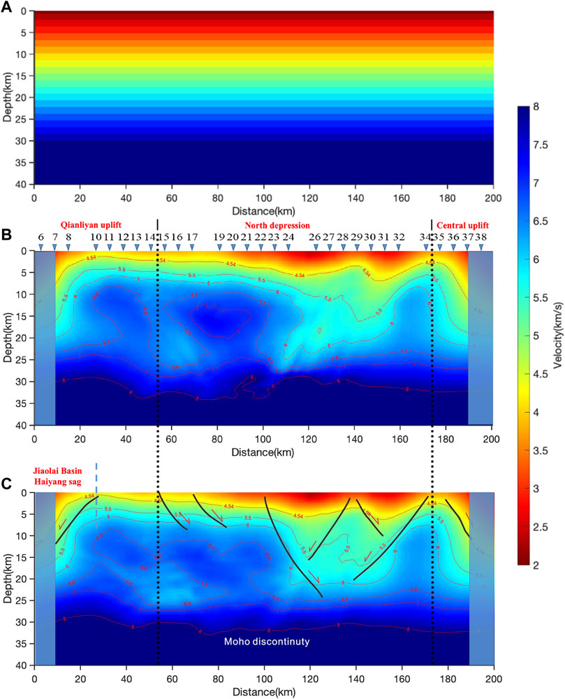
FIGURE 4. (A) Initial velocity model, (B) tomographic inversion results of first-arrival traveltimes and their gradients, and (C) tomographic inversion results of traveltimes and their gradients of first-arrival wave joint-reflected waves.

First, 284 groups of first-arrival traveltimes and their gradients were employed for tomographic inversion. In the inversion process, the multiscale strategy was utilized to continuously subdivide the grid. Subsequently, the grid was divided every 20 iterations. After 60 iterations, we derived the inversion result with a grid size of 1 × 0.375 km (Figure 4B). Then, 395 groups of the reflection traveltimes and their gradients were added for joint tomographic inversion. The weight coefficient of the first-arrival data item is 0.4, and the reflection data item is 0.6. Using the same initial model and iteration parameters as the first-arrival inversion, the final inversion result of the reflection data is presented in Figure 4C. By tracking the RMSE (root mean square error) of position, slope, and traveltime of the source and receiver pairs in the iterative process, it is found that the inversion process is convergent. Comparing Figure 4B with Figure 4C, the tomographic inversion results using only the first-arrival data are fundamentally consistent with the joint inversion results above 15 km. However, the two inversion results for the mid-deep velocity below 15 km differ. The joint tomographic inversion result is of higher quality than the tomographic inversion result of the first-arrival data.

Based on the joint tomographic inversion results in Figure 4C, the shallow velocity of the model between OBS14 and OBS36 is low, and the velocity on both sides is higher than that in the middle. The tectonic boundary between the Qianliyan Uplift, Northern depression, and Central Uplift is clearly given, which is consistent with the tectonic boundary’s location distribution in Figure 1. Moreover, the velocity model above a depth of 5 km (e.g., the velocity contour of 4.54 km/s) also reflects the distribution of secondary structures. OBS22, OBS23, and OBS24 are located on the North Branch of the Northern depression’s Western bulge, and OBS29 is on the South Branch of the Northern depression’s Western bulge.

The basement of the Jiaolai Basin comprises Late Archean–Late Proterozoic metamorphic rocks, which extensively crop out on the basin’s northern and southern sides. Primarily, the sedimentary rock series is composed of the Lower Cretaceous Laiyang Group and Qingshan Group, as well as the Upper Cretaceous Wangshi Group. In particular, the Laiyang Group is primarily deposited by river lake facies clastic sediments, which are intercalated with dolomitic shale and a small number of pyroclastic rocks. In addition, the Qingshan Group is an intricate series of volcanic, pyroclastic, and typical sedimentary rocks. Finally, the Wangshi Group is made of river lake facies clastic rocks mixed with mudstone and pyroclastic rocks. For each set of strata, the thickness can reach several thousand meters, which are either in parallel unconformity or angular unconformity. A small amount of the Paleogene strata is present in numerous regions, such as in the Pingdu Sag, and a small number of Quaternary deposits are distributed in the basin’s northwestern area (Qiu et al., 2011). Based on the joint inversion results itemized in Figure 4C in the Qianliyan Uplift area, because the high-velocity body below the Haiyang Sag of the Jiaolai Basin has a large-scale extension to the Qianliyan Uplift, the low-velocity Cretaceous strata directly cover the Sulu Orogenic Belt’s pre-Sinian metamorphic rock basement.

As the central body of the lower Yangtze paraplatform, the SYS Basin is a multicycle superimposed basin of Meso-Paleozoic marine basins and Meso-Cenozoic continental basins based on the pre-Nanhua fold metamorphic crystalline basement. More specifically, the SYS Basin can be categorized into three structural layers from the bottom to the top: the Nanhua Early Middle Triassic marine strata as the lower structural layer, a late Cretaceous Paleogene half-graben lacustrine deposit in the middle, and Neogene–Quaternary depression-type fluvial facies and marine continental facies clastic sediment as the upper layer (Zhang et al., 2014; Zhao et al., 2019b). The inversion results in Figure 4C show that in the Central Uplift area, due to the strong erosion since the Indo-China movement, the low-velocity Neogene–Quaternary strata in the upper structural layer are directly overlaid by the Mesozoic and Paleozoic carbonate formations in the lower structural layer. As a result, a strong difference in the formation velocity in the shallow part of the two regions exists. At depths of 5 km–20 km in the model, a large area of a relatively low-velocity anomaly from OBS22 to OBS32 in the Northern depression is observed. This indicates that under the Meso-Cenozoic continental strata of the middle and upper structural layers of the Northern depression, the geological situation of an exceedingly thick lower structural layer can be found in the Meso-Paleozoic marine strata.

The Moho discontinuity in Figure 4C is approximately determined according to the 8 km/s velocity contour. Its depth in the study area ranges from 28 km to 32 km. In the Qianliyan Uplift, affected by the strong subduction collision orogeny between the Yangtze block and the North China block during the Indosinian period, the Moho discontinuity fluctuates to a great extent, but in other regions, it fluctuates only at a very low level.

Conclusion

With the OBS2013 line in the SYS, this study combines the phase-shift wave-field extrapolation and the principle of reciprocity, and the traveltimes and their gradient picking of the local coherent events of sparse OBS data are realized. Simultaneously, the crustal velocity structure and the undulating shape of the Moho discontinuity in the SYS are revealed by joint tomographic inversion of reflected and refracted seismic waves. Accordingly, the crustal velocity structure substantiated that the high-velocity body in the deep Haiyang Sag of the onshore Jiaolai Basin extends to the SYS’s Qianliyan Uplift area at a large scale. It is also worth noting that the low-velocity Cretaceous strata directly cover the pre-Sinian metamorphic rock basement of the Sulu Orogenic Belt, and the thick Meso-Paleozoic marine strata are preserved under the Meso-Cenozoic continental strata in the Northern depression. Finally, the fluctuation characteristics of the Moho discontinuity in a depth range of 28–32 km in the study area are further characterized.

Data availability statement

The raw data supporting the conclusion of this article will be made available by the authors, without undue reservation.

Author contributions

FM adapted the algorithm, analyzed the data, and wrote the manuscript; FH provided fruitful discussions on the tomographic results. TL provided fruitful discussions on the algorithm; ZW provided the original OBS2013 data and technical guidance. JZ conceived and revised the manuscript. All authors listed have made a substantial, direct, and intellectual contribution to the work, and approved it for publication.

Funding

This work was supported by the Shandong Provincial Natural Science Foundation (China) (Grant No. ZR2019MD001).

Conflict of interest

The authors declare that the research was conducted in the absence of any commercial or financial relationships that could be construed as a potential conflict of interest.

Publisher’s note

All claims expressed in this article are solely those of the authors and do not necessarily represent those of their affiliated organizations, or those of the publisher, the editors, and the reviewers. Any product that may be evaluated in this article, or claim that may be made by its manufacturer, is not guaranteed or endorsed by the publisher.

References

Alerini, M., Traub, B., Ravaut, C., and Duveneck, E. (2009). Prestack depth imaging of ocean-bottom node data. Geophysics 74 (6), WCA57–63. doi:10.1190/1.3204767

CrossRef Full Text | Google Scholar

Billette, F., Bégat, S., Podvin, P., and Lambaré, G. (2003). Practical aspects and applications of 2d stereotomography. Geophysics 68 (3), 1008–1021. doi:10.1190/1.1581072

CrossRef Full Text | Google Scholar

Billette, F., and Lambar, G. (1998). Velocity macro-model estimation from seismic reflection data by stereotomography. Geophys. J. Int. 135 (2), 671–690. doi:10.1046/j.1365-246X.1998.00632.x

CrossRef Full Text | Google Scholar

Cui, X., Li, H., Hu, Y., Hong, L., and Li, Q. (2007). Wavefield continuation datuming using a near surface model. Appl. Geophys. 4 (2), 94–100. doi:10.1007/s11770-007-0014-y

CrossRef Full Text | Google Scholar

Garret, M., Rebecca, L., and Jan, S. (2012). Imaging the shallow crust with teleseismic receiver functions. Geophys. J. Int. 191, 627–636. doi:10.1111/j.1365-246X.2012.05615.x

CrossRef Full Text | Google Scholar

Gazdag, J. (1978). Wave equation migration with the phase-shift method. Geophysics 43, 1342–1351. doi:10.1190/1.1440899

CrossRef Full Text | Google Scholar

Jin, C., and Zhang, J. (2018). Stereotomography of seismic data acquired on undulant topography. Geophysics 83 (4), U35–U41. doi:10.1190/geo2017-0411.1

CrossRef Full Text | Google Scholar

Lambare, G., Alerini, M., Baina, R., and Podvin, P. (2004). Stereotomography: A semi-automatic approach for velocity macromodel estimation. Geophys. Prospect. 52 (6), 671–681. doi:10.1111/j.1365-2478.2004.00440.x

CrossRef Full Text | Google Scholar

Li, T., Liu, J., and Zhang, J. (2019). A 3D reflection ray-tracing method based on linear traveltime perturbation interpolation. Geophysics 84 (4), T181–T191. doi:10.1190/geo2018-0119.1

CrossRef Full Text | Google Scholar

Li, X., Li, S., Suo, Y., Somerville, I., Huang, F., Liu, X., et al. (2017). Early Cretaceous diabases, lamprophyres and andesites-dacites in Western Shandong, North China Craton: Implications for local delamination and Paleo-Pacific slab rollback. J. Asian Earth Sci. 160, 426–444. doi:10.1016/j.jseaes.2017.08.005

CrossRef Full Text | Google Scholar

Liu, J., and Zhang, J. (2022). Joint inversion of seismic slopes, traveltimes and gravity anomaly data based on structural similarity. Geophys. J. Int. 229 (1), 390–407. doi:10.1093/gji/ggab478

CrossRef Full Text | Google Scholar

Liu, L., Hao, T., Lu, C., Wu, Z., Zheng, Y., Wang, F., et al. (2021). Crustal deformation and detachment in the Sulu Orogenic Belt: New constraints from onshore-offshore wide-angle seismic data. Geophys. Res. Lett. 48, e2021GL095248. doi:10.1029/2021GL095248

CrossRef Full Text | Google Scholar

Liu, L., Hao, T., Lue, C., You, Q., Pan, J., Wang, F., et al. (2015). Crustal structure of bohai sea and adjacent area (north China) from two onshore–offshore wide-angle seismic survey lines. J. Asian Earth Sci. 98, 457–469. doi:10.1016/j.jseaes.2014.11.034

CrossRef Full Text | Google Scholar

Peacock, K., and Treitel, S. (1969). Predictive deconvolution: Theory and practice. Geophysics 34 (2), 155–169. doi:10.1190/1.1440003

CrossRef Full Text | Google Scholar

Prieux, V., Lambaré, G., Operto, S., and Virieux, J. (2013). Building starting models for full waveform inversion from wide-aperture data by stereotomography. Geophys. Prospect. 61, 109–137. doi:10.1111/j.1365-2478.2012.01099.x

CrossRef Full Text | Google Scholar

Qiu, X., Zhao, M., Ao, W., Lu, C., Hao, T., You, Q., et al. (2011). OBS survey and crustal structure of the southwest sub-Basin and nansha block, south China sea. Chin. J. Geophys.-CH. 54 (12), 3117–3128. doi:10.3969/j.issn.0001-5733.2011.12.012

CrossRef Full Text | Google Scholar

Schleicher, J., Costa, J., Santos, L., Novais, A., and Tygel, M. (2008). On the estimation of local slopes. Geophysics 74 (4), 25–33. doi:10.1190/1.3063968

CrossRef Full Text | Google Scholar

Wan, T. (2012). The tectonics of China: Data, maps and evolution. Berlin, Heidelberg: Springer-Verlag. ISBN: 978-3-642-11866-1, 978-3-642-11868-5.

Google Scholar

Yang, K., Fan, J., Cheng, J., Ma, Z., and Wang, L. (2007). An integrated wave equation datuming scheme for the overthrust data based on the one-way extrapolator. Seg. Tech. Program Expand. Abstr. 26 (1), 3124. doi:10.1190/1.2792938

CrossRef Full Text | Google Scholar

Zhang, H., Qiu, X., Wang, Q., Huang, H., and Zhao, M. (2021). Data processing and seismic phase identification of OBS converted shear wave in the Xisha Block. Chin. J. Geophys.-CH. 64 (11), 4090–4104. doi:10.6038/cjg2021O0293

CrossRef Full Text | Google Scholar

Zhang, X., Yang, J., Li, G., and Yang, Y. (2014). Basement structure and distribution of Mesozoic-Paleozoic marine strata in the South Yellow Sea basin. Chin. J. Geophys.-CH. 57 (12), 4041–4051. doi:10.6038/cjg20141216

CrossRef Full Text | Google Scholar

Zhao, W., Wang, H., Shi, H., Xie, H., Zheng, Y., Chen, S., et al. (2019a). Crustal structure from onshore-offshore wide-angle seismic data: Application to northern sulu orogen and its adjacent area. Tectonophysics 770, 228220. doi:10.1016/j.tecto.2019.228220

CrossRef Full Text | Google Scholar

Zhao, W., Zhang, X., Wang, H., Chen, S., Wu, Z., Hao, T., et al. (2020). Characteristics and noise combination suppression of wide-angle ocean bottom seismography (OBS) data in shallow water: A case study of profile OBS2016 in the south Yellow Sea. Chin. J. Geophys.-CH. 63 (6), 2415–2433. doi:10.6038/cjg2020N0360

CrossRef Full Text | Google Scholar

Zhao, W., Zhang, X., Zou, Z., Wu, Z., Hao, T., Zhang, Y., et al. (2019b). Velocity structure of sedimentary formation in the South Yellow Sea Basin based on OBS data. Chin. J. Geophys.-CH. 62 (1), 183–196. doi:10.6038/cjg2018L0623

CrossRef Full Text | Google Scholar

Zou, Z., Liu, K., Zhao, W., Liu, H., Zhou, H., Meng, X., et al. (2016). Upper crustal structure beneath the northern south yellow sea revealed by wide-angle seismic tomography and joint interpretation of geophysical data. Geol. J. 51 (S1), 108–122. doi:10.1002/gj.2847

CrossRef Full Text | Google Scholar