 Baixue Li
 Xueying Wang
 Feifei Zhang1,2
95% of researchers rate our articles as excellent or good
Learn more about the work of our research integrity team to safeguard the quality of each article we publish.
Find out more
ORIGINAL RESEARCH article
Front. Earth Sci. , 09 January 2023
Sec. Economic Geology
Volume 10 - 2022 | https://doi.org/10.3389/feart.2022.1036281
This article is part of the Research Topic Advances in Multi-Physics Multi-Component Fluid Transport and Multi-Scale Geophysical Modeling in Unconventional Oil and Gas Reservoir - Volume II View all 4 articles
Because of the existence of cuttings in the flow, the pressure loss in the wellbore can increase significantly. Minimization of the flow pressure loss greatly benefits the drilling process. This work investigates the most important factors to the pressure loss in the wellbore during the hole cleaning process. It is found that, for the solid–liquid, two-phase flow, the fluid flow rate is not always proportional to annular pressure loss as the single-phase flow. The mechanisms behind this effect are studied, and a mechanistic model based on the solid–liquid, two-phase flow is proposed to simulate the hole cleaning process and predict the critical fluid flow rate, which gives the minimum pressure loss in the wellbore. The effect of the inclination angle, fluid rheological parameters, annulus geometry, and the rate of penetration on the critical value are investigated by using the proposed model. Results show that the critical flow rate value increases as the inclination angle increases under 60° and decreases once the inclination angle goes beyond 60°. The critical flow rate increases as the fluid viscosity and the wellbore geometry increase. This proposed model can be used to minimize the pressure loss in the wellbore in the given operational conditions and optimize the drilling parameters.
For a successful extended reach well (ERW) drilling operation, accurate control of the equivalent circulation density (ECD) is essential. High ECD can lead to a series of drilling problems, such as lost circulation. ECD is the sum of equivalent static density (ESD) and additional pressure loss caused by the fluid flow. ECD controlling does not decrease the ESD but optimizes the flow rate to reduce the additional pressure loss. Considering the effect of the wellbore and drill string geometry, drilling fluid, rheology, flow rates, and drilling operations in calculating ECD are necessary. Several studies have been conducted to investigate the modeling of ECD. Luo and Peden (1987) predicted that annulus pressure loss would decrease with the increase in drill pipe rotation because of the fluid shear-thinning theory. Hemphill and Ravi (2007) focused on the effect of the drill string rotational speed on the predicted ECD. Hemphill and Ravi (2011) simplified their model in another study. The presence of the tool joint changes the annulus geometry between the drill pipe and casing/hole, resulting in strong turbulence and fluid acceleration that generate additional viscous dissipation and pressure losses. Jeong and Shah (2004) investigated the effect of the tool joint on annular pressure loss with a non-rotating drill pipe. Simoes et al. (2007) focused on the influence of tool joints on wellbore hydraulics, which was conducted considering different wellbore and tool-joint geometries, and presented results for a theoretical study conducted through computational fluid dynamics (CFD) techniques to evaluate the influence of the tool joints on the ECD for different wellbore geometries, drilling fluids, and flow rates. A high-temperature/high-pressure condition is very common in deep wells. Therefore, the effect of temperature and pressure on fluid rheology cannot be ignored. Rommetveit and Bjorkevoll (1997) presented the effects of pressure and temperature on fluid rheology for typical HPHT wells. Osisanya and Harris (2005) employed the Bingham plastic model to express the rheological behavior of the drilling fluids studied, with rheological parameters expressed as functions of temperature and pressure. Although many theoretical and experimental studies have been conducted on fluid flow through annuli to predict the ECD, most undermine or simply ignore the effect of cuttings.
Both field applications and laboratory studies show that cuttings in the wellbore can significantly affect the pressure gradient (Coley and Edwards, 2013; Zhang et al., 2014). The effects of cuttings on ECD are contributed by three aspects: the mud hydrostatics pressure, the solid phase in the mud, and the frictional pressure loss in the annulus (Yao et al., 2022). Zhang et al. (2015) were the first to investigate the relationship between the annulus pressure loss and hole cleaning in depth. Experimental results show that annulus pressure loss does not always rise with the increase in the flow rate in extended reach wells and horizontal wells. There is a critical value due to the existence of cuttings below which the annular pressure loss decreases with the increase in the flow rate. Once beyond the critical value, the annulus pressure loss begins to increase, as shown in Figure 1.
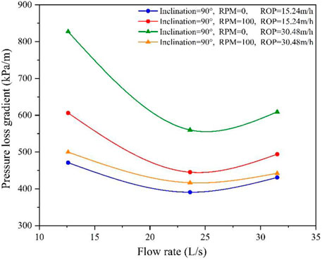
FIGURE 1. Effect of the flow rate on annulus pressure loss.
The existence of the critical value (inflection point) shown in Figure 1 is the combined effect of cuttings on the drilling fluid density, effective annulus flow area, and friction coefficient. First, the mixing of cuttings and drilling fluid changes the effective density of the flow in the wellbore. Second, in the inclined or horizontal section, cuttings settle at the lower part of the annulus, which reduces the effective annulus flow area and increases the drilling fluid velocity, thereby increasing the friction loss in the wellbore. Third, the cuttings bed increases surface roughness. At low flow rates, cuttings accumulate in the wellbore due to gravity. The formation of cutting beds reduces the annulus equivalent flow area and improves the drilling fluid density and friction coefficient, which results in high annulus pressure loss. However, with the increase in the flow rate, cuttings are suspended into the drilling fluid and circulated out of the well. Consequently, the annulus pressure loss decreases with the decrease in the height of the cuttings bed. Once the flow rate exceeds a certain value (the turning point in Figure 1), the increase in friction loss becomes more important, the influence of cuttings concentration and cuttings bed becomes minor, and annulus pressure loss increases as the flow rate increases.
This study proposes a method to determine the hole cleaning criteria and optimize drilling parameters by minimizing the ECD in deviated wells during drilling. The relationship between hole cleaning and annulus pressure loss is established based on cuttings transport mechanistic models. The effects of major factors such as the well inclination angle, annulus size, cuttings density, ROP, and rheological parameters of drilling fluid are investigated. Moreover, a workflow is presented to optimize the drilling parameters.
Depending on the inclination of the wellbore and the operational conditions, the cuttings may form different flow patterns in the wellbore (Zhang et al., 2015). Based on the flow patterns, a set of mechanistic models is developed to cover all the scenarios during the drilling process.
The solid phase can distribute in various geometrical configurations for the flow of solid–liquid mixtures in the annulus with different inclination angles. The geometrical configurations, which are also called flow patterns, identified flow patterns to be dominated by two factors: solid settling and solid re-suspension. Four flow patterns were presented for the solid–liquid, two-phase flow in annulus geometry in drilling applications, covering the entire inclination range (from vertical to horizontal), as shown in Figure 2.
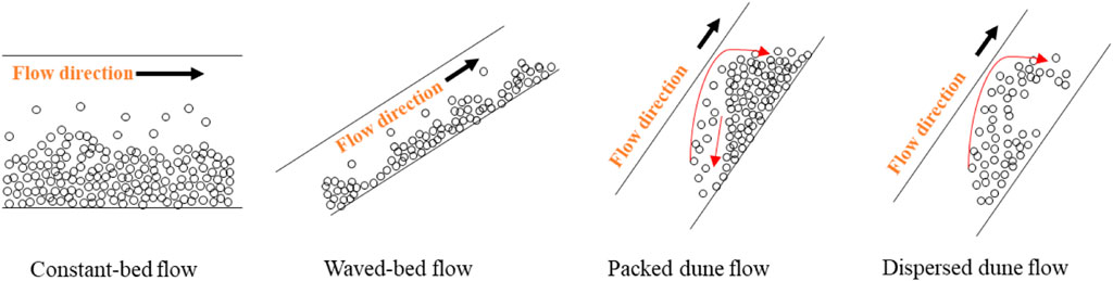
FIGURE 2. Cuttings flow patterns for the entire inclination range (Zhang et al., 2015).
A dimensionless flow pattern map is developed from the experimental results, as shown in Figure 3. The horizontal axis of the flow pattern map is the reciprocal of an extended Froude number (Fr). In this application, the Froude number is modified using Eq. 1. The vertical axis of the flow pattern map is a dimensionless number (DPG) related to the pressure loss of the mixture flow in the annulus, which is expressed by Eq. 2:
where
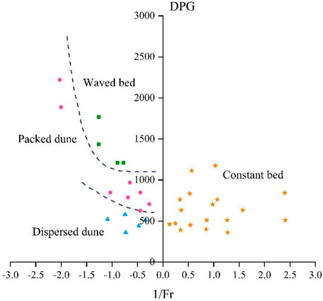
FIGURE 3. Flow pattern map (Zhang et al., 2015).
The constant-bed flow commonly occurs in horizontal or highly inclined wells, and a three-layer model is applied to describe this pattern. In the model, the cross section of the annulus can be divided into three parts based on the distribution of cuttings, as shown in Figure 4.
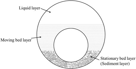
FIGURE 4. Three-layer model geometry.
The assumptions of the model are listed as follows:
1) There are no cuttings in the upper liquid layer.
2) The moving bed layer is a mixture of cuttings and fluid, and there is no slip between the fluid and the particles.
3) The fluid velocity in the moving bed layer is constant.
4) In a control volume, the height of the stationary bed layer is constant in the direction of the borehole axis, and the porosity of the cuttings bed is constant.
5) The cuttings diameter is uniform, and all the cuttings are assumed to be spherical.
The conservation of mass of the solid phase is as follows:
where
The conservation of mass of the liquid phase is as follows:
where
For the upper dispersed layer, the momentum equation is as follows:
where
For the moving bed layer,
where
For the stationary bed layer, the criterion keeping it from moving is that the driving force acting on the bed is less than the resistance. Eq. 7 is the case where the driving force acting on the bed is less than the resistance, and the stationary bed is at rest. Eq. 8 is the case of cuttings moving upward. At this time, the friction force between the moving bed layer and wellbore wall is the driving force, which is located on the left side of the equation. The driving force overcomes the resistance and presents an upward movement state, and some cuttings move to the moving bed layer as follows:
where
When the cuttings bed is stationary, we have six unknowns:
When the cuttings bed is in motion, we have seven unknowns:
As the well inclination angle decreases, the cuttings in the stationary smooth cutting bed slide download. The sliding leads to the appearance of waves in the cuttings bed. The waved-bed flow is composed of three parts: the flow region, stationary cuttings slug region, and sliding cuttings film region (Figure 5).
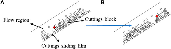
FIGURE 5. Original segment model.
A simplified segment model is applied to simulate the cuttings transport for this flow pattern. In this model, it is assumed that the cuttings between two neighboring slugs are fully dispersed, and there is no cuttings film, as shown in Figure 6.
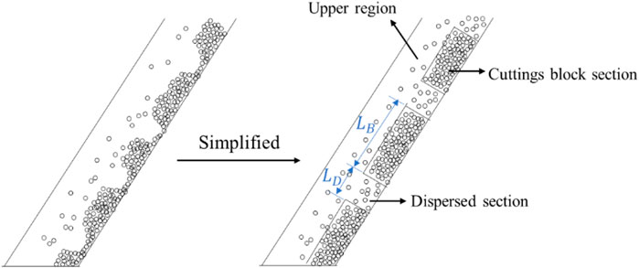
FIGURE 6. Simplified segment model.
In the segment model, the following assumptions are proposed:
1) In the upper part of the annulus, the cuttings are fully dispersed, meaning the cuttings concentration is homogeneous.
2) In the lower part of the annulus, the cuttings block region is stationary, and the dispersed regions move forward at a constant velocity. The cuttings are fully dispersed in the dispersed region. The mass exchange rate between the dispersed and block regions is constant. The sizes of the block and the dispersed regions are uniform along the test section.
3) The pressure gradient in the upper region is the same as that in the dispersed region and the cuttings block region. Because of the pressure gradient, there is fluid flow in the cuttings block. The flow is insignificant compared to the flow in the upper part of the annulus and the dispersed region. Thus, the fluid flow in the cuttings block is neglected.
4) The drill pipe rotation is not considered in this model.
5) The cuttings diameter is uniform, and all the cuttings are assumed to be spherical.
6) There is no slip between the particles and the liquid.
The conservation of mass for the solid phase is as follows:
where
For the liquid phase,
The momentum equation for the upper part is as follows:
where
The momentum equation for the dispersed region is as follows:
where
The momentum equation for the solid block region is as follows:
and
where
In the model, we have six unknowns:
At the low inclined position and high flow rate conditions, the cuttings in the wellbore may get totally dispersed. The local cuttings concentration in the wellbore is directly related to the cuttings slip velocity.
The superficial liquid velocity
and the superficial cuttings velocity
where
The feeding in the cuttings concentration
The cross-section average in situ cuttings concentration
where
The average slip velocity between the drilling fluid and cuttings
where
The mixture equation is as follows:
where
Substituting Eq. 20 and Eq. 21 into Eq. 19, we obtain
The pressure gradient for the dispersed model is obtained using standard drilling hydraulic models, by replacing the pure drilling fluid velocity with the mixture velocity and the fluid density with the new mixture density of the local cuttings and fluid:
where
According to the experimental observation, the cuttings roll forward rather than slide forward on the surface of the cuttings bed. Therefore, the fluid velocity near the cuttings bed is the critical velocity of cuttings rolling. In the mechanistic model, the average velocity above the cuttings bed can be considered as the average velocity of the mixed layer. There is a cuttings exchange between cuttings beds and mixed beds. The cuttings of the mixed layer are continuously settled to the cuttings bed because of gravity. Meanwhile, the cuttings are re-suspended to the mixed layer due to the effect of turbulent suspension and particle uplift. The mixed layer cuttings concentration profile is obtained by comparing the upward re-suspension and downward deposition. The closure equations proposed in conjunction with boundary conditions can avoid multi-solution problems and simplify the model-solving process.
The solution mentioned previously requires the critical velocity of cuttings movement, namely, the minimum fluid velocity that enables the cuttings to move continuously forward. Particles begin to roll on the cuttings bed surface at first in highly inclined wells. Figure 7 is the free body diagram of a random rolling particle on the surface of the cuttings bed.
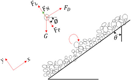
FIGURE 7. Particle rolling.
When the particle began to roll on the surface of the cuttings bed, the sum of the moment on the particle caused by all the forces acting on the particle
where
In order to make the particle roll on the cuttings bed,
where
For intermediate inclined wells, the cuttings can be re-suspended to the flow more easily than rolling on the bed surface. To lift the particle away from the cuttings bed, the sum of the force in the y direction should be larger than zero, which means
Therefore,
where
When the particle leaves the cuttings bed, FN goes to zero. Moreover, the critical velocity to suspend the particle is as follows:
For the control volume shown in Figure 8,
where
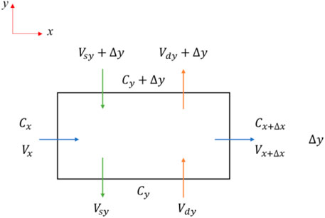
FIGURE 8. Cuttings diffusion in a control volume.
For the fully developed flow,
where
For non-horizontal wells, the settling velocity is
where
In this case, because of the large cuttings, the shear-induced diffusion can be neglected, and only turbulent diffusion is considered. By rearranging Eq. 32,
where the Schmidt number
The downward settling velocity is as follows:
The boundary conditions are as follows: at the top of the moving layer, the cuttings concentration is 0. At the bottom of the moving layer, the cuttings concentration is the same as the packed cuttings bed concentration.
The model is solved by using a numerical method, and detailed procedures are shown as follows:
1) Input calculation data, such as the wellbore geometry, flow rate, and fluid rheological parameters.
2) Assume the height of the cutting bed from zero, and assume the annular pressure gradient
3) Judge the flow pattern for the solid–liquid, two-phase flow, and calculate the Froude number using Eq. 1 and DPG using Eq. 2.
4) Calculate the wet perimeters and areas of the annular geometry (details available in previous work (Zhang et al., 2015)).
5) Calculate the velocity of every layer using Eqs. 28 and 34.
6) Update the cuttings concentration and bed height using Eqs. (3), 4.
7) Calculate the shear stress, Reynolds number, and friction coefficient using the equations in Appendix B.
8) Calculate the annular pressure gradient using Eqs. 5–8.
9) Compare the calculated results, assume that
10) Plot the ECD against the flow rate to establish the minimum ECD curve and then obtain the minimum flow rate.
In order to verify the reliability of the model, the results are compared with the experimental data published in the literature (Zhang et al., 2015; Zhang, 2015). The accuracy and reliability of the model are verified by the comparative test data on hole inclination, rotary speed, and ROP.
The comparison results are shown in Figures 9–12. At a low flow rate (12.6 L/s), the predicted results are in good agreement with the experimental data. The average difference between predictions and experimental results is about 5%. With the increase in the flow rate, the model matches the experimental data well.
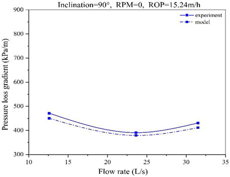
FIGURE 9. Pressure loss gradient at 90°, 15.24 m/h, and 0 RPM.
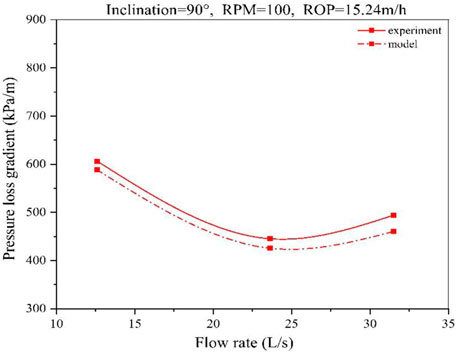
FIGURE 10. Pressure loss gradient at 90°, 15.24 m/h, and 100 RPM.
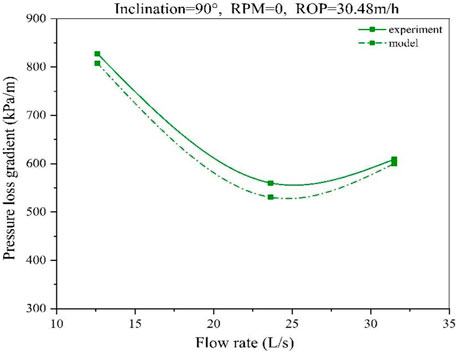
FIGURE 11. Pressure loss gradient at 90°, 30.48 m/h, and 0 RPM.
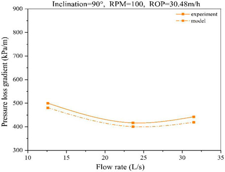
FIGURE 12. Pressure loss gradient at 90°, 30.48 m/h, and 100 RPM.
In order to show the influence of cuttings on annulus pressure loss more clearly under the conditions of different sections, inclined angle, flow rate, ROP, and drilling fluid parameters, the annulus pressure loss in a single section under different conditions is calculated and analyzed.
In this case, rotary speed and ROP are assumed to be constants, 100 RPM and 30.48 m/h, respectively. The relationship between the flow rate and annulus pressure loss is shown in Figure 13 as inclination changes.
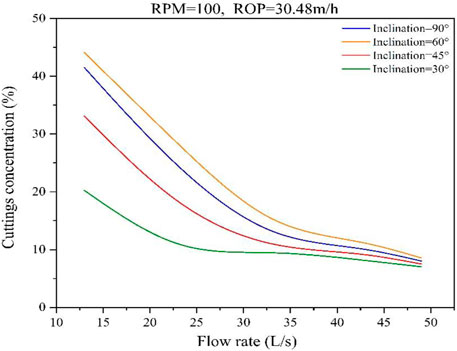
FIGURE 13. Effect of the inclination angle on the cuttings concentration.
When the flow rate and inclination angle are both small, the annulus pressure loss is specifically high. However, the annulus pressure loss decreases obviously with the hole inclination increasing, as shown in Figure 14, which is caused by the concentration of cuttings at different inclination positions shown in Figure 13. For all inclination positions, there is a turning point for the pressure gradients as the flow rate increases. The flow rate value for the turning points increases as the inclination angle increases below 60° and decreases beyond 60°, which is consistent with the cuttings concentration results shown in Figure 13. It can be indicated that the flow rate of the turning point is proportional to the efforts required to clean the wellbore.
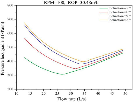
FIGURE 14. Effect of the inclination angle on pressure loss.
In this case, both fluids are power-low flow, and the density is 1,000 kg/m3. The first fluid behavior index (n) is 0.814, and the consistency coefficient (K) is 0.065 pasn. The second fluid n is 0.72, and K is 0.0254 pasn. Figure 15 shows the calculation results of the variation of the annulus pressure loss of the two different drilling fluids with the flow rate change in a deviated well with 100 RPM and an ROP of 30.48 m/h.
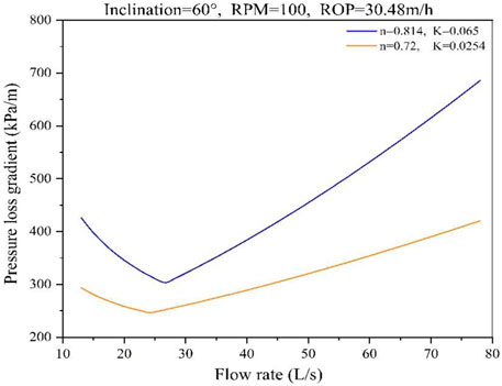
FIGURE 15. Effect of rheological parameters on pressure loss.
Figure 15 shows that there is little effect on the fluid flow index; the greater the fluid consistency coefficient, the greater the viscosity is. Therefore, the annulus pressure loss is larger. Moreover, the increase in the fluid viscosity reduces the value of the critical flow rate.
In this case, the first geometry is 230*114 (mm), and the second is 244*114 (mm). Results are shown in Figure 16. From the diagram, we can find that the annulus pressure loss decreases with the increase in annulus geometry, but the critical flow rate is adverse. The increase in the annulus geometry reduces the annulus velocity and the consumption of drilling fluid friction resistance. However, the decrease in the flow rate reduces the carrying capacity of the drilling fluid, which increases the critical value.
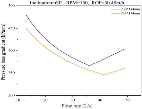
FIGURE 16. Effect of annulus geometry on pressure loss.
Figure 17 shows the variation of annulus pressure loss with flow rate change in a deviated well after ROP changed. The rotary speed is 100 RPM. The consistency coefficient (K) of the drilling fluid is 0.065 pasn, and the behavior index (n) is 0.72. It can be found from the diagram that the annulus pressure loss and the critical flow rate both increase with the increase in the ROP. Because ROP increases, the number of suspended cuttings and the height of the cuttings bed in the annulus increase, resulting in an increase in the annulus velocity and the fluid average density. Therefore, the annulus pressure loss curve in Figure 17 shifts to the upper right.
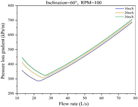
FIGURE 17. Effect of ROP on pressure loss.
Based on this model, combined with the data on well A, the whole wellbore cleaning optimization method of extended reach wells is analyzed. The casing program is shown in Figure 18 and can be divided into vertical and horizontal sections. The basic data include the following: the length of the vertical section is 2,902 m; the outer diameter of the casing is 244.5 mm; the length of the horizontal section is assumed to be 3,000, 3,500, and 4,000 m; the diameter of the bits is 215.9 mm; the outer of the drill pipe is 127 mm; the rotary speed is 100 RPM; and the ROP is 15.24 m/h. The drilling fluid is power-low flow with a density of 1,000 kg/m3, a behavior index (n) of 0.814, and a consistency coefficient (K) of 0.065 pasn. The cuttings used in the case are sandstone. The cuttings density is 2,667 kg/m3, the average diameter is 3 mm, and the packed porosity is 0.36.
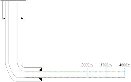
FIGURE 18. Structure of the wellbore.
The bottom hole pressure under different flow rates in open hole drilling is shown in Figure 19A. Because of the presence of cuttings and friction, the annulus pressure loss in the flowing condition is larger than hydrostatic pressure. The details of the pressure near the bottom hole region are shown in Figure 19B. The optimal flow rate in this condition is about 36 L/s. A lower flow rate leads to high solid concentration in the well, which increases the bottom hole pressure; a higher flow rate leads to more friction loss, which also increases the bottom hole pressure.
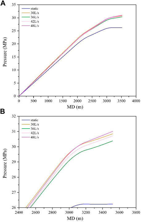
FIGURE 19. (A) Wellbore pressure profile. (B) Wellbore pressure profile for the near-bottom region.
The cuttings concentration profile in the wellbore is shown in Figure 20. The cuttings concentration decreases with the increase in the flow rate. At 36 L/s, the cuttings concentration is less than 5% in the vertical part of the well, which satisfies the requirements of traditional wellbore cleaning. In the inclined and horizontal sections of the wellbore, slight cuttings deposition is acceptable during drilling.
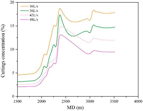
FIGURE 20. Solids’ concentration profile in the wellbore.
In most drilling applications, it is necessary to minimize the pressure loss caused by friction and cuttings in the annulus. The pressure drop in the annulus is not always proportional to the flow rate. At a low flow rate, the concentration of cuttings in the wellbore is relatively high, which results in a high-pressure drop. In these cases, increasing the flow rate can reduce the cuttings concentration significantly, which actually reduces the total pressure drop. In the low cuttings concentration condition, the influence of cuttings on pressure loss is very small. In these cases, increasing the flow rate will lead to a significant increase in friction loss, which also increases the bottom hole pressure. Therefore, at the optimum flow rate of 36 L/s, the pressure loss in the annulus is the smallest.
Figure 21 shows the calculation results of the annulus pressure loss changes with the variety of flow rates at different horizontal sections, which further proves the optimum flow rate.
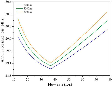
FIGURE 21. Effect of horizontal section length on pressure loss.
Through experiments and theoretical research, the following conclusions can be drawn:
1) The annulus pressure loss is closely related to the cuttings concentration. Without effective hole cleaning, many cuttings accumulate in the annulus and significantly impact pressure loss.
2) There is a critical flow rate for the relationship value between the flow rate and annulus pressure loss. When the flow rate is less than the critical value, the annulus pressure loss decreases with the increase in the flow rate. When the flow rate exceeds the critical value, the annulus pressure loss begins to increase with the increase in the flow rate.
3) The critical value varies with the rheological parameters of the drilling fluid, ROP, hole inclination, and the annulus size.
4) According to the requirements of drilling technology, a new method for hole cleaning optimization in extended reach wells by minimizing the ECD is presented, which can be used to optimize drilling parameters and minimize the ECD during drilling ERD wells.
The raw data supporting the conclusions of this article will be made available by the authors, without undue reservation.
BL verified the model. XW analyzed and summarized the application process of the minimum ECD model method for extended-reach wellbore cleaning. FZ analyzed the flow pattern and mechanical model. XW derived the closure equations. YW analyzed the influence of multiple factors on the cuttings concentration and pressure loss gradient in a single-well section. YW analyzed the cuttings concentration, pressure profile, and annular pressure loss distribution in the whole section of the real case well.
This work was supported by the National Natural Science Foundation of China (Grant no. 51874045) and the Hubei Provincial Science and Technology Agency (Grant no. 2019CFA093).
The authors declare that the research was conducted in the absence of any commercial or financial relationships that could be construed as a potential conflict of interest.
All claims expressed in this article are solely those of the authors and do not necessarily represent those of their affiliated organizations or those of the publisher, the editors, and the reviewers. Any product that may be evaluated in this article, or claim that may be made by its manufacturer, is not guaranteed or endorsed by the publisher.
Coley, C. J., and Edwards, S. T. (2013). “The use of A long string annular pressure measurements to monitor solids transport and hole cleaning,” in Paper SPE 163567 presented at the SPE/IADC Drilling Conference, Amsterdam, The Netherlands, 5-7 March 2013.
Hemphill, T., and Ravi, K. (2007). “Field validation of drill pipe rotation effects on equivalent circulating density,” in paper SPE 110470 presented at the SPE Annual Technical Conference and Exhibition in Anaheim, Anaheim, California, 11-14 November 2007.
Hemphill, T., and Ravi, K. (2011). “Improved prediction of ECD with drill pipe rotation,” in Paper IPTC 15424 presented at International Petroleum Technology Conference, Bangkok, Thailand, 15-17 November 2011.
Jeong, Y., and Shah, S. (2004). “Analysis of tool joint effects for accurate friction pressure loss calculation,” in Paper SPE 87182 presented at IADC/SPE Drilling Conference, Dallas, Texas, 2-4 March 2004.
Luo, Y., and Peden, J. M. (1987). “Flow of drilling fluids through eccentric annuli,” in Paper SPE 16692 presented at the SPE Annual Technical Conference and Exhibition, Dallas, Texas, 27-30 September 1987.
Osisanya, S. O., and Harris, O. O. (2005). “Evaluation of equivalent circulating density of drilling fluids under high pressure/high temperature conditions,” in Paper SPE 97018 presented at SPE Annual Technical Conference and Exhibition, Dallas, Texas, 9-12 October 2005.
Ozbayoglu, E. M. (2002). “Cuttings transport with foam in horizontal and highly-inclined wellbore,” (Tulsa, Oklahoma, USA: The University of Tulsa). Ph.D. Dissertation.
Rommetveit, R., and Bjorkevoll, K. S. (1997). “Temperature and pressure effects on drilling fluid rheology and ECD in very deep wells,” in Paper SPE 39282 presented at SPE/IADC Middle East Drilling Technology Conference, Bahrain, 23-25 November 1997.
Simoes, S. Q., Miska, S. Z., Takach, N. E., et al. (2007). “The effect of tool joints on ECD while drilling,” in Paper SPE 106647 presented at Production and Operations Symposium, Oklahoma City, Oklahoma, U.S.A, 31 March-3 April 2007.
Yao, Y., Qiu, Y., Cui, Y., Wei, M., and Bai, B. (2022). Insights to surfactant huff-puff design in carbonate reservoirs based on machine learning modeling. Chem. Eng. J. 451, 138022. doi:10.1016/j.cej.2022.138022
Zhang, F., Miska, S., and Yu, M. (2014). “Application of real-time solids monitoring in well design, annulus pressure control and managed pressure drilling,” in Paper presented at the 2014 AADE Fluids Technical Conference and Exhibition, Houston, Texas, USA, 15-16 April 2014.
Zhang, F., Miska, S., Yu, M., Evren, M., and Takach, N. (2015). Pressure profile in annulus: Solids play a significant role. J. Energy Resour. Technol. 137, 34–45. doi:10.1115/1.4030845
Keywords: drilling hydraulics, ECD, extended reach well, hole cleaning, mechanistic models
Citation: Li B, Wang X, Zhang F, Wang X, Wang Y and Wang Y (2023) A mechanistic model for minimizing pressure loss in the wellbore during drilling by considering the effects of cuttings. Front. Earth Sci. 10:1036281. doi: 10.3389/feart.2022.1036281
Received: 04 September 2022; Accepted: 20 September 2022;
Published: 09 January 2023.
Edited by:
Wenhui Song, China University of Petroleum, ChinaReviewed by:
Wang Chen, China University of Petroleum, ChinaCopyright © 2023 Li, Wang, Zhang, Wang, Wang and Wang. This is an open-access article distributed under the terms of the Creative Commons Attribution License (CC BY). The use, distribution or reproduction in other forums is permitted, provided the original author(s) and the copyright owner(s) are credited and that the original publication in this journal is cited, in accordance with accepted academic practice. No use, distribution or reproduction is permitted which does not comply with these terms.
*Correspondence: Xueying Wang, d2FuZ3h5QHlhbmd0emV1LmVkdS5jbg==
Disclaimer: All claims expressed in this article are solely those of the authors and do not necessarily represent those of their affiliated organizations, or those of the publisher, the editors and the reviewers. Any product that may be evaluated in this article or claim that may be made by its manufacturer is not guaranteed or endorsed by the publisher.
Research integrity at Frontiers
Learn more about the work of our research integrity team to safeguard the quality of each article we publish.