 Wei Cheng1,2
 Xiaowen Zhang1,2Juan Jin1,2Jiandong Liu1,2*Weidong Jiang1,2Guangming Zhang1,2
 Shihuai Zhang3*Xiaodong Ma3
- 1Research Institute of Petroleum Exploration & Development, PetroChina, Beijing, China
- 2Key Laboratory of Oil & Gas Production, CNPC, Beijing, China
- 3Department of Earth Sciences, ETH Zürich, Zürich, Switzerland
The stress-strain relationship in shales is generally time-dependent. This concerns their long-term deformation in unconventional reservoirs, and its influence on the in situ stress state therein. This paper presents an experimental investigation on the time-dependent deformation of the Longmaxi shale gas shale. A series of creep experiments subject the shale samples to long-term, multi-step triaxial compression. It is found that the shale samples exhibit varying degrees of time-dependent deformation, which can be adequately described by a power-law function of time. The experimental results establish the relationship between the elastic Young’s modulus and viscoplastic constitutive parameters, which are different from previous those derived from North American shales. Based on this viscoplastic constitutive model, the stress relaxation and the differential stress accumulation over geologic time scales can be estimated. It is found that linear elasticity substantially overestimates the differential stress accumulation predicted in the context of viscoplastic relaxation. The characterized viscoplasticity and stress relaxation are of vital importance for various geomechanical problems in shale reservoirs.
1 Introduction
The boom in unconventional plays in recent decades requires deeper understanding of the geomechanical properties and in situ stress characteristics of shale gas reservoirs. The refined understanding of the rock properties and in situ stress facilitates reservoir evaluation, drilling, wellbore stability, and well stimulation (Britt and Schoeffler, 2009; Britt, 2012; Zheng et al., 2018; Clarke et al., 2019; Wang et al., 2019; Zoback and Kohli, 2019). The mechanical properties of shales are significantly different from those of common rock types (e.g., sandstones and carbonates) characterized by heterogeneity, time-dependency and anisotropy. Challenges remain when conventional concepts and models (such as linear elasticity) are applied to infer the geomechanical properties and in situ stress in shale reservoirs.
Shales typically consist of rich compliant components, e.g., clay minerals and total organic carbon content (TOC), which promote significant time-dependent deformation. Such time-dependence may affect a variety of mechanical processes in situ. For instance, hydraulic fractures opened by proppants can eventually close over time, leading to reservoir permeability loss and thus production reduction (Guo and Liu, 2012; Li and Ghassemi, 2012; Rybacki et al., 2017). The time-dependent deformation of shales is often invoked as one of the main mechanisms for the reservoir compaction or surface subsidence (Hagin and Zoback, 2007; Chang et al., 2014; Musso et al., 2021). In addition, the time dependence of shales has also been closely related to the evolution of the state of in situ stress. For example, in a normal or normal/strike-slip faulting regime, it has been observed that the least principal stress (quantifying the frac gradient) can increase markedly in a viscoplastic formation, rendering a more isotropic state of stress than that in the more elastic/brittle formations above and below (Warpinski and Teufel, 1989; Sone and Zoback, 2014b; Ma and Zoback, 2017). Plausibly due to viscoplastic stress relaxation (Yang et al., 2015; Xu et al., 2019), the increased magnitude of the least principal stress may act as a stress barrier with a higher frac gradient, limiting the propagation of vertical hydraulic fractures. Predicting the variations of the least principal stress at different depths can facilitate the optimization of drilling and the control of fracture propagation (hydraulic fracturing and seismicity mitigation). However, it has been demonstrated that the observed variations of the least principal stress within shale formations cannot be well explained by the frictional equilibrium concept (Townend and Zoback, 2000; Sone and Zoback, 2014b; Ma and Zoback, 2020). Therefore, quantifying the time-dependent response of shales is of vital importance to in situ stress prediction and other geomechanical applications.
In order to investigate the time-dependent response of shales, a lot of uniaxial and triaxial creep experiments have been carried out (Chang and Zoback, 2009; 2010; Li and Ghassemi, 2012; Sone and Zoback, 2014a; Yang and Zoback, 2016; Rassouli and Zoback, 2018). It is found that creep can be enhanced, to different extent, in the presence of high differential stress, high content of compliant components, and water and loaded in the direction perpendicular to bedding orientation. In order to describe the laboratory-derived creep behavior, the empirical laws for rocks, soils, and other solids can generally be used, including power-law, logarithmic, exponential, and hyperbolic functions (Gupta, 1975; Findley et al., 1976; Karato, 2008; Paterson, 2012). Among them, the power-law model has been successfully used to quantify the linear viscous behavior of North America shales under primary creep stage and its long-term effect on the in situ state of stress (Sone and Zoback 2014a; Sone and Zoback 2014b; Yang et al., 2015; Ma and Zoback, 2020). Considering the different tectonic environments, however, it is not clear if the empirical relations derived from North America shales can be directly applied to other shale types, such as the Wufeng-Longmaxi shale investigated in this paper.
In this study, we performed a series of multi-step creep experiments on the shale samples from the Longmaxi formation, a major unconventional play in southwestern China (Zou et al., 2015; Dong et al., 2018). Based on the laboratory triaxial creep experiments, the time-dependent behavior of the Longmaxi shale samples was investigated considering the effect of hydrostatic loading, differential stress, and deformational anisotropy. Utilizing the theory of linear viscoelasticity, the time-dependent constitutive relation was established for the Wufeng-Longmaxi shale samples. According to the experimental data, a new empirical relation was proposed to relate the constitutive parameters to the elastic properties. Then the laboratory-derived viscoplastic stress relaxation response was extrapolated, facilitating an estimation of the in situ stress over geologic time scales.
2 Shale samples and laboratory methodology
2.1 Longmaxi shale lithofacies—Taking Well 1 as an example
Shale cores tested in this study are from three vertical appraisal wells, referred to as Well 1, 2, and 3, respectively. The three wells are all located in a shale gas reservoir at the southern margin of the Sichuan Basin, China. Tectonically, the shale gas reservoir is located in the Changning anticline area, which is essentially a large basement fault-bend fold. Its tectonic location is the transition zone between the south Sichuan low-slow fold belt and the Daliangshan-Daloushan fault fold belt (He et al., 2019). Although characterized by complex structural deformation in the geologic history, the in situ stress data, mostly from World Stress Map (Hu et al., 2017; Heidbach et al., 2018; Kong et al., 2021) and focal mechanism inversions of historic earthquakes (Lei et al., 2019), consistently indicate the regional NW-W trend of the SHmax and the reverse faulting/strike-slip stress environment in this region (Ma et al., 2022). Among the three wells, a series of integrated well logs are available from the depth of 1950–2300 m in Well 1, characteristic of the regional geology and reservoir lithofacies. It has been confirmed that the clay-rich Wufeng-Longmaxi formations are the target of the shale gas play, showing the potential to yield economic hydrocarbon production.
In Figure 1, the integrated geophysical logs corresponding to part of the Wufeng-Longmaxi formations and the underlying Baota Formation are shown (depth: 2195–2265 m). The gamma ray logs show high values (>100 GAPI) within the reservoir depths, indicating the high content of clay (Figure 1A). After entering the Baota formation, the gamma ray value decreases abruptly to a low level, consistent with the diminishing clay shown in compositional log in Figure 1B. Overall, the clay-rich Wufeng-Longmaxi formations have a marked contrast in mineralogy to the underlying carbonate-rich Baota formation. The lower Longmaxi formation is further divided into several lithofacies according to their characteristic physical properties, which is evident in terms of mineral composition (e.g., clay content) and mechanical properties (e.g., sonic log derived Young’s modulus and Poisson’s ratio). The stratigraphic column in Figure 1, from top to bottom, shows the successive lithofacies of the Longmaxi formation: Longmaxi-I2 (“L-I2”), L-I1^4, L-I1^3, L-I1^2, and L-I1^1. The variations in mineral composition and physical properties among the lithofacies clearly show that the Longmaxi shale is highly heterogenous. To further study the mechanical behavior of the Longmaxi shale, several shale samples were retrieved within the target formation in each well. Figure 1 shows the extracted core depths in Well 1.
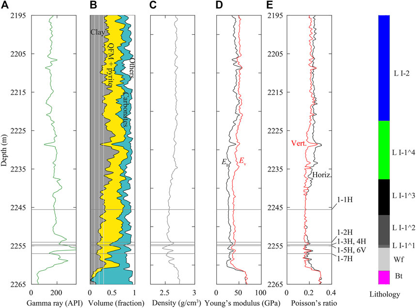
FIGURE 1. Integrated geophysical logs of Well 1: (A) Gamma ray; (B) Element Capture Spectroscopy (ECS); (C) Density; (D) Sonic log derived Young’s modulus; (E) Sonic log derived Poisson’s ratio. The coring depths of seven shale samples from Well 1 are shown with “H” and “V” denoting horizontal and vertical samples, respectively. For reference, the stratigraphic column is also shown where “L”, “Wf”, and “Bt” denote Longmaxi, Wufeng, and Baota formations, respectively.
2.2 Sample preparation and description
The shale cores from the three wells were prepared into cylindrical samples with nominal diameter of 25 mm and nominal length of 50 mm. These samples have cylindrical axes either perpendicular or parallel to the bedding planes, which are referred to as vertical (denoted as “V”) and horizontal (denoted as “H”) samples, respectively. Note that samples from the same lithofacies have significantly different depths across wells, as shown in Table 1, indicating a highly inclined formation in the shale gas play. For each well, there is one pair of vertical and horizontal samples cored from the same depth, i.e., 1–5H and 1–6V in Well 1, 2–1V and 2–2H in Well 2, and 3–2H and 3–3V in Well 3. Those samples have also been analyzed for the mineral composition using powder X-ray diffraction (XRD) method after the creep experiments. In Figure 2, the mineral composition results are summarized as squares in a ternary plot with clay, QFP (quartz, feldspar, pyrite), and carbonate content, which are further provided in Table 1. The shown samples, except for 1–7H, are from the same lithofacies. From Figure 2, the ternary diagram indicates that samples 1–5H and 1–6V are relatively clay-rich, and 2–1V and 2–2H are relatively silicate-rich. For sample 1–7H, its mineral composition departs significantly from that of samples 1–5H and 1–6V, although its coring depth is only 3 m deeper. For comparison, the mineral composition data in Figure 1B are also plotted as dots in the ternary diagram. Apparently, the compositional log via Element Capture Spectroscopy (ECS) indicates systematically higher clay contents and lower QFP contents (volume percentage) than those of the samples from Well 1. Such inconsistency may be attributed to the differences in scale and measurement methods. Before performing the creep experiments on these samples, two shale samples (S1 and S2) without detailed coring information were tested for calibration purposes.
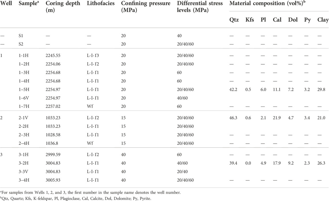
TABLE 1. Mineral composition and experimental data of the shale samples used in the multi-step creep experiments. “H” and “V” denote horizontal and vertical samples, respectively.
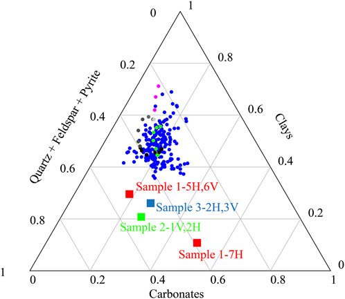
FIGURE 2. Ternary plot of the mineral composition (in volume fraction) for several representative samples (squares) tested in this study. “H” and “V” denote horizontal and vertical samples, respectively. For reference, the mineral composition of different lithofacies in Well 1 is shown as dots with colors indicated by the stratigraphic column in Figure 1.
2.3 Experimental procedures
Multi-step creep experiments were performed using a servo-controlled triaxial apparatus to investigate the time-dependency of the shale samples. Previous studies on North America shales reveal that the confining pressure effect seems to be absent or slightly affecting creep rates (e.g., Sone and Zoback, 2014a). In this study, the confining pressure applied to the samples from each well is approximately estimated according to the coring depth (Table 1) and the shale density (2.5–2.7 g/cm3), although overpressure might be present in the reservoir depths (He et al., 2019). In general, three differential stress levels (20, 40, and 60 MPa) were designated to subject the samples to various stress conditions pertinent to the in situ effective differential stress. In what follows, we take the multi-step creep experiments on Sample S2 as an example to present the experimental procedure. As shown in Figure 3A, the creep response of Sample S2 was measured at three differential stress levels (20, 40, and 60 MPa) under the confining pressure of 20 MPa.
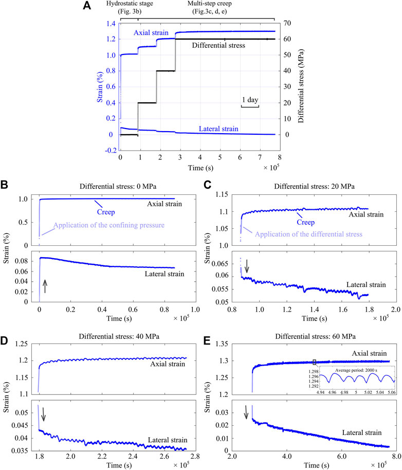
FIGURE 3. (A) Differential stress and axial/lateral strains evolving with time during the multi-step creep experiment (Sample: S2, confining pressure: 20 MPa). For the first three steps, the stress was held for about 1 day (24 h), while the stress for the last step was held for about 6 days. Detailed information of the strains evolving with time is shown in (B–E): (B) hydrostatic stage, (C–E) differential stress stages with differential stresses of 20, 40, and 60 MPa, respectively. Arrows represent the increase or decrease of the lateral strain during the “instantaneous” loading. Note that data with light color denote the application of the confining pressure or differential stresses. Also note the scale difference for the axial and lateral strain in (B–E).
Specifically, the sample was first subject to confining pressure. The increase of confining pressure lasted around 400 s to reach the prescribed level. The sample then stayed in the hydrostatic stage for ∼24 h to reach its thermal equilibrium. Differential stress Pdiff was then raised consecutively to three levels (i.e., 20, 40, and 60 MPa) at a loading rate of 2 MPa/min in the subsequent three steps. For the first two steps, the differential stress (20 and 40 MPa) was held constant for ∼24 h. For the last step, differential stress (60 MPa) was held constant for about 6 days. During the creep process, the applied differential stress was recorded by the pressure transducer and the strains were measured by the linear variable differential transducer (LVDT). In Figure 3A, the recorded differential stress and strains of Sample S2 are shown as a function of time during the multi-step creep experiment.
Note that, the in situ stress in the upper crust is typically limited by the rock frictional strength (Townend and Zoback, 2000), which is generally much lower than the ultimate compressive strength of the intact rock. To characterize the time-dependence of the shale samples, the applied differential stresses are less than 50% of the ultimate strength. Under such relatively low stress levels, we can obtain the viscoplastic behavior of the shale samples while preventing the transition into tertiary creep. In Table 1, the applied confining pressures and differential stresses of the tests in this study are detailed.
3 Experimental results
3.1 Mechanical characteristics during the multi-step creep experiments
During each experiment, the shale sample experienced “instantaneous” deformation and “long-term” creep in each step. From Figure 3A, three main features can be observed: 1) significant deformation takes place under hydrostatic loading; 2) creep strain is most prominent in the axial direction; and 3) creep induces dilatant lateral strain that cannot be overlooked. In the hydrostatic stage, as presented in Figure 3B, contraction (positive) occurs in both the axial and lateral directions. As in the subsequent creep stages, the deformation in the axial direction is more pronounced than that in the lateral direction when increasing the confining pressure to the prescribed value. While the hydrostatic state is maintained for a period of ∼24 h, the axial strain is almost constant while the lateral strain first decreases (dilates) and then reaches a constant value. This may be due to the intrinsic anisotropy of the samples or the different methods for measuring the axial and lateral strains. Based on this observation, it is argued that the sample should stay in the hydrostatic stage for sufficiently long period (e.g., 12 h as suggested by Figure 3B) to reach a state of equilibrium in terms of deformation and temperature.
Similarly, the shale sample in the differential stress stage also shows a combination of instantaneous elastic response and time-dependent creep response. In Figures 3C–E, it can be observed that, upon each differential stress step, most of the axial strain (light blue data) occurs during the ‘instantaneous’ application of the differential stress. In contrast, the lateral strain first decreases in response to the “instantaneous” loading and then undergoes more deformation at an almost constant rate during the creep stage. In addition, when the differential stress is held, both the axial and lateral strains show significant “cyclic” fluctuations, which may be due to the loading system artefact during the long-time creep period or the temperature fluctuations in the testing environment. In Figure 3E, the close-up of a time interval around 5×10⁵ s clearly shows the details of the data fluctuations. Regression to the data yields an average period of about 2000 s.
3.2 Comparative observations between shale samples
In Section 3.1, anisotropy can be observed for a single sample from the different strain responses in the axial and lateral directions. In this section, we further compare the mechanical responses of different samples under the hydrostatic stage and differential stress stage. In Figure 4, the axial strain data of several representative shale samples under hydrostatic stage are shown. These samples can be divided into different pairs, and each pair are from the same depth, i.e., 1–3H and 1–4H (2254.68 m), 1–5H and 1–6V (2254.97 m), 2–1V and 2–2H (1033.23 m), 3–2H and 3–3V (3004.83 m). Under hydrostatic condition, samples 1–3H and 1–4H, featuring the same coring depth and orientation, display considerably different response to the “instantaneous” loading of the confining pressure, indicative of significant heterogeneity of these shale samples. For the effect of sample orientation, it is observed that the horizontal sample 1–5H shows more significant amount of axial strain than the vertical sample 1–6V. In contrast, the horizontal samples show less axial strain than the vertical samples for Well 2 and Well 3. As reported by previous studies, e.g., Wong et al. (2008), shale samples are typically stiffer in the horizontal direction (bedding parallel) than in vertical direction (bedding perpendicular), consistent with their assumptions being transverse isotropy materials. Therefore, it is generally expected more pronounced creep behavior for vertical samples. Comparison between 1 and 5H and 1–6V shows the mechanical features of shale samples are not always consistent with a transverse isotropy model, which may be due to its complex microstructure. As shown in Figure 5, the two thin-sections taken from the same depth as samples 1–5H and 1–6V exhibit either the abundance of flaking clay minerals or abundant calcite, which strongly support the high heterogeneity of the Wufeng-Longmaxi shale. It can thus be inferred that the horizontal sample 1–5H contains more clay minerals than the vertical sample 1–6V, leading to a more compliant horizontal sample as also suggested by the logging-derived Young’s modulus shown in Figure 1D. As anther result, the compositional difference could mask the orientation effect predicted by the transverse isotropy model.
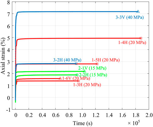
FIGURE 4. Axial strain responses of the samples from three wells under hydrostatic conditions. For each curve, the sample name and the corresponding confining pressure are explicitly indicated. For comparison, each pair of the samples are from the same depth, i.e., 1–3 H and 1–4 H, 1–5 H and 1–6 V, 2–1 V and 2–2 H, 3–2 H and 3–3 V (see Table 1 for more details).
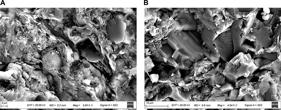
FIGURE 5. SEM micrographs of two thin-sections corresponding to the same depth as the samples 1–5 H and 1–6 V. (A) Micrograph shows flake illite, clastic grains, pelletized pyrite, organics, and micro-pores. (B) Micrograph shows the abundance of calcite wrapped by clay minerals, and inter-/intra-grain pores.
As aforementioned, the “instantaneous” response of the sample to the differential stress may also be largely elastic. In Figure 6, we plot the cumulative differential stress versus the cumulative axial strain after each differential stress step. It appears that the main difference between the two samples of a pair is the axial strain accumulated in the hydrostatic stage. After applying the differential stress, all samples regardless of the well and depth show similar stress-strain relations. Specifically, for each sample, the relationship between the differential stress and the cumulative axial strain is approximately linear, plausibly justifying the linear elastic behavior of the sample under the relatively low differential stresses. The dependence of the cumulative axial strain on differential stress can then be quantified by the slope, which is effectively the Young’s modulus. For each sample, the applied several differential stress steps yield individual values of Young’s modulus. In addition, combining all differential stress steps, an average Young’s modulus can be further obtained as indicated by the dashed line in Figure 6. In Table 2, the Young’s modulus values of each sample are summarized.
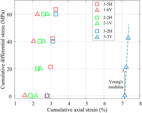
FIGURE 6. Relationship of the cumulative differential stress and total axial strain for three pairs of shale samples. Each pair of samples were retrieved from the same depth.
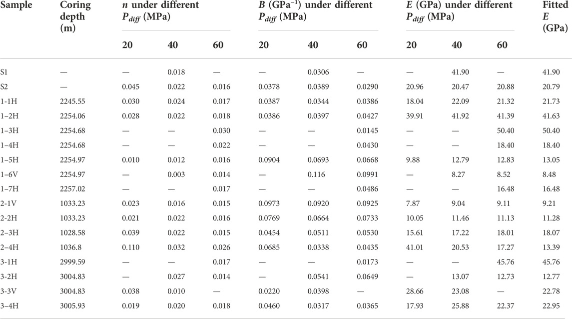
TABLE 2. Power-law constitutive parameters for Longmaxi shale sample.
3.3 Viscoplastic constitutive relationship
In the framework of linear viscoelastic theory (see Appendix A), we can quantitatively calculate the creep compliance J(t) describing the time-dependent strain response to a unit input (Heaviside step) of differential stress. Specifically, J(t) can be obtained by dividing the measured strain by the magnitude of differential stress in laboratory investigations. In Appendix B, we have tested different functions to fit the experimental results. It is found that the power-law function and logarithmic function can best fit the experimental data. As explained by Sone and Zoback (2014a), the creep compliance generally shows self-similar characteristics in time, which can be well described by both functions. In particular, the power-law function is simple and capable of predicting long-term creep behavior, which has been extensively used in previous studies (Sone and Zoback, 2014a; Yang and Zoback, 2014; Yang et al., 2015; Rassouli and Zoback, 2018; Xu et al., 2019; Mandal et al., 2021).
In Figure 7, the creep compliance data for the three differential stress steps of Sample S2 are plotted versus time in the log-log space. Each set of data shows an increasing trend with the logarithm of time. As with the strain data in Figure 3, the creep compliance data also feature fluctuations with decreasing degree with time. When the holding time is sufficiently long, the compliance data starts to show a linear trend. For the same sample under different differential stresses, it displays remarkably different creep compliance responses by the individual slopes. Quantitatively, the experimental data can be fitted by the widely-used power-law function:
where B and n are viscoplastic constitutive parameters. As illustrated in Figure 7, each set of the creep compliance data can be well fitted by a straight line based on linear regression. Accordingly, n is the slope of the line and B is related to the intercept of the vertical axis. In the multi-step creep experiments, note that, the application of differential stress is not ideally “instantaneous”. However, compared with the long creep period, the application of differential stress can be approximately regarded as an instantaneous Heaviside step. Therefore, it is general to discard the initial portion of the experimental data associated with the stress application when determining the creep compliance function

FIGURE 7. Relationships of creep compliance (J) and time (t) for three differential stress levels (20, 40, 60 MPa) shown in the log-log space (Sample: S2, confining pressure: 20 MPa). The grey data is the first 1000 s which is not considered in the linear regression. Red solid lines are the fitted results.
3.4 Constitutive parameters of the shale samples
The determined viscoplastic constitutive parameters (B and n) listed in Table 2 are now plotted in Figure 8. Comparison between each well shows that these samples, although collected from different wells and depths, fall within a similar range of n value, i.e., 0 to 0.04. For values of B, however, Samples S1 and S2 and Well 3 samples possess relatively lower B values, whereas the B values of Well 2 samples span a higher range (0.04–0.1) and Well 1 samples possess the widest range of B values (0.01–0.12). In addition, both Well 1 samples and Well 2 samples show that the vertical samples have higher B values and lower n values than horizontal samples, indicating anisotropy in their viscoplastic properties. However, the samples from Well 3 do not show apparent anisotropy from the laboratory results.

FIGURE 8. Summary of the constitutive parameters of all shale samples.
According to Eq. 1, it could be interpreted that B is the creep compliance corresponding to the initial 1 s of creep deformation (Sone and Zoback, 2014a). Essentially, B is intimately related to the instantaneous elastic modulus of the shale sample. In previous studies (Sone and Zoback, 2014a; Yang et al., 2015), the relationship between 1/B and the calculated Young’s modulus E of a variety of shales consistently shows a one-to-one correlation, despite some dispersion. To examine the relationship between 1/B and E of the Longmaxi shale, the experimental data are plotted in Figure 9. Excluding the data (Samples S1 and 1–2H) above the diagonal line, the Young’s modulus E derived from the multi-step creep experiments is approximately 0.7 times of 1/B, which is different from the empirical relations of the shales from North America (Sone and Zoback, 2014a). From Figures 8, 9, it can be seen that the vertical samples are more compliant than the horizontal samples, except for Well 3 samples, which is generally consistent with the theoretical prediction of the transverse isotropy model.
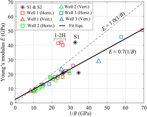
FIGURE 9. Relationship of 1/B and Young’s modulus derived from the multi-step creep experiments.
The power exponent n is a parameter associated with time-dependency, describing the relative contribution of the creep strain to the total strain observed at a given time. In other words, a larger value of n corresponds to more pronounced creep behavior. As an end-member, the value of n = 0 corresponds to an elastic behavior independent of time. Another interesting observation is that, for samples from Wells 1 and 2, higher values of B are accompanied by lower values of n. In other words, samples with lower Young’s modulus have a lower creep tendency. In Figure 10, this trend is further observed by plotting the correlation between Young’s modulus and the constitutive parameter n. By contrast, data of several North American shales (Sone and Zoback, 2014a) show that n generally decreases with E. The observation of the studied shale samples appears to be counterintuitive, since one would generally expect larger amount of creep deformation for samples with lower Young’s modulus due to more compliant components (Yang et al., 2015; Rassouli and Zoback, 2018; Xu et al., 2019). As indicated by Figure 5B, the abundance of stiff minerals (e.g., calcite) is likely accompanied by the abundant micro-pores, which may often contain fluids as suggested by the overpressure in the Wufeng-Longmaxi formation. Consequently, it is inferred that the abundance of stiff minerals contributes to high Young’s modulus as a short-term response. At the same time, pore reduction/collapse and drainage could take place over a long time, leading to significant creep deformation as a long-term response. Such an inference could plausibly explain the observation that the stiffer samples feature more significant creep behavior, which, however, still warrants further investigation.
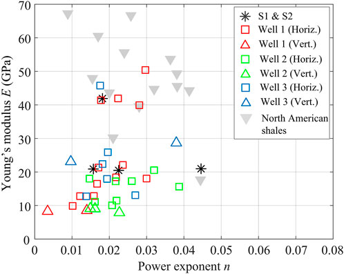
FIGURE 10. Correlation between Young’s modulus and the constitutive parameter n for the studied shale samples. For comparison, data of shales from North American (Sone and Zoback, 2014a) are also plotted.
4 Long-term effect of viscoplasticity
4.1 Expected stress relaxation of the shale samples
Following the theory of linear viscoelasticity, we first obtain the relaxation modulus function by performing Laplace transform operations (Lakes, 2009; Sone and Zoback, 2014a):
Eq. 2 implies that 1/B is effectively the Young’s modulus at t = 1 s,
With the relaxation modulus function, we can further calculate the stress response with time based on Eq. (A2). Assuming a constant strain rate
where
In Figure 11, the variation of the stress relaxation factor with the constitutive parameter n for different time scales ranging from several days (0.01 years) to years and to millions of years. For all time scales, the stress relaxation factor decreases continuously with the increase of n, quantifying the tendency of viscous relaxation. For a certain value of n, the unrelaxed stress decreases with time scales and the effect of time gradually diminishes. For example, the difference between 10 Myr and 200 Myr for any value of n is much smaller than that between 0.01 years and 1 year. In other words, a significant amount of stress relaxes within an initial short period of time, which is insignificant compared with the geologic time scales. As indicated by Eq. 3, as long as the accumulated strain
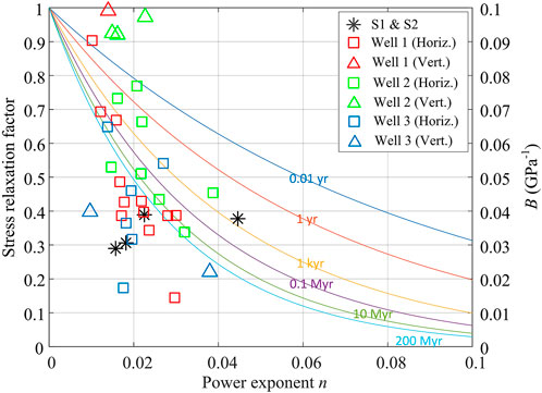
FIGURE 11. Stress relaxation factor as a function of the power exponent n for several time scales from several days up to 200 millions of years (Myr). For comparison, the constitutive parameters of all the samples are plotted.
4.2 Estimation of differential stress accumulation over geological time scales in situ
To estimate the accumulation of differential stress over a certain period of time, a constant strain rate of 10–19 and a deformation duration of 150 Myr are prescribed. Note that it is not easy to constrain a reasonable tectonic strain for the studied shale gas play located near the southern margin of the Sichuan Basin due to the complex geologic and tectonic history. The strain rate and deformation duration are only used for illustrative purpose.
As shown in Figure 9, most of the horizontal samples have the Young’s modulus (Ehori) of 10–30 GPa. Over the deformation duration of 150 Myr, the accumulated differential stresses for the horizontal samples are expected to be between 6.8 and 20.3 MPa in the absence of viscoelastic relaxation. Taking the time-dependency of shales into consideration, the differential stress accumulated over the deformation duration is estimated and shown as contours in Figure 12. The predicted magnitude of the differential stress for all samples ranges from 3 up to 20 MPa. Note that, the values where the contours intercept with the horizontal axis (n = 0) correspond to the elastic stress accumulation without viscous relaxation. For a certain B value, stress relaxation becomes more pronounced as n increases, indicating less accumulation of the differential stress.
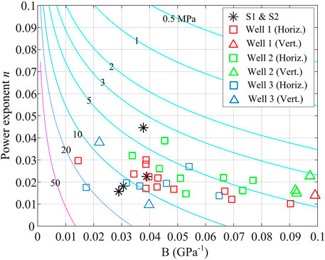
FIGURE 12. Stress accumulation (contours) as a function of the constitutive parameters (B and n). In the calculation, a constant strain rate of 10–19 and a deformation duration of 150 Myr are assumed. The constitutive parameters of all studied samples are also plotted.
For most of the horizontal samples, the magnitude of the cumulative differential stress is predicted to be 3–10 MPa. Compared with the differential stress in the absence of viscoelastic relaxation, the stress reduction after 150 Myr is about 50%, which is similar to the percentage corresponding to 200 Myr as shown in Figure 11. In other words, the stress reduction rate decreases significantly with time. Therefore, if a perfectly isotropic state of in situ stress is observed in at the reservoir depths, two main reasons could be present: 1) The shale experiences a sufficiently long period of viscoplastic deformation; 2) other mechanisms, such as frictional slips (Zhang and Ma, 2021) and overpressure (Miller et al., 2004), can also be operative so that a more isotropic stress state is attainable over a shorter time scale.
5 Concluding remarks
In this study, a series of laboratory multi-step creep experiments were performed on several Longmaxi shale samples to investigate their time-dependent deformation properties. It is found that studied shale samples exhibit varying degrees of time-dependent strain response, which can be adequately described by a power-law function of time. Based on this viscoplastic model, we extrapolated the stress relaxation of the tested samples and calculated the differential stress accumulation over geologic time scales. Specifically, the following conclusions can be obtained:
1) Under the applied differential stress levels (20–60 MPa), the instantaneous response of all samples is approximately linear and elastic.
2) The studied samples, collected both from the same well and from different wells, exhibit varying degrees of time-dependent deformation. The time-dependent strain response can be well described by a power-law function of time with only two parameters (B and n).
3) From the experimental results, it is found that Samples S1 and S2 and Samples from Well 3 possess relatively lower values of B, whereas the B values of Well 2 samples are higher. For the constitutive parameter n, all samples fall within the same ranges (0–0.04). Samples from Wells 1 and 2 show that the vertical samples have higher values of B and lower values of n, indicating the anisotropy in the viscoelastic properties. However, samples from Well 3 do not show apparent anisotropy from the laboratory results.
4) The elastic Young’s modulus E correlates with both constitutive parameters (B and n). As indicated by the experimental data, it is found that E ≈ 0.7 (1/B). For the correlation between E and n, it is found that higher E generally corresponds to higher n, which means that a stiffer sample (with higher Young’s modulus) tends to exhibit more pronounced time-dependent deformation. Such observation is counterintuitive since one would expect larger creep deformation for samples with lower Young’s modulus due to more compliant components. Therefore, further investigation is required in the future, particularly for the microstructure of the samples.
5) The degree of stress relaxation over certain time periods is positively related to the constitutive parameter n. For a certain value of n, the unrelaxed stress decreases with time but the effect of time gradually diminishes so that a significant amount of differential stress relaxes in the initial short period of time.
6) Linear elasticity is not adequate to predict the differential stress accumulation over time. The predicted differential stress accumulation is much larger in the absence of viscoelastic relaxation. As an example, for most of the horizontal samples, the magnitude of differential stress is predicted to be 3–10 MPa over 150 Myr at a constant strain rate of 10–19. In contrast, the accumulated differential stress is predicted to be 6.8–20.3 MPa by linear elasticity.
To summarize, our laboratory experiments reveal the tendency of the long-term deformation of the Longmaxi shale. The viscoplastic parameters, characterizing the long-term behavior, can be correlated with the elastic Young’s modulus, quantifying the transient behavior that can be measured in situ with logs and ex situ in the laboratories. The viscoplastic properties of the Longmaxi shale can be readily extrapolated to the in situ stress estimation over geologic time scales, facilitating a variety of geomechanical applications in the development of unconventional reservoirs. Specifically, characterizing the in situ state of stress, especially the “bed-to-bed” lithology-controlled stress variations, is critical to optimizing horizontal well trajectory, improving hydraulic fracturing effectiveness, and controlling fracture propagation. The workflow presented here for the Longmaxi shale reservoir can be potentially applied to other unconventional plays.
Data availability statement
The original contributions presented in the study are included in the article/Supplementary Material, further inquiries can be directed to the corresponding authors.
Author contributions
WC, XZ, JJ, JL, WJ, and GZ contributed in conceiving this research, laboratory experiments, original draft preparation. SZ and XM contributed in formal analysis, validation, and reviewing.
Funding
This project is sponsored by Research Institute of Petroleum Exploration and Development (RIPED), China National Petroleum Corporation (CNPC) through an international collaborative grant (No. 17064). Open access funding provided by ETH Zurich. This study is partly supported by the Swiss National Science Foundation (Grant no.182150).
Acknowledgments
We thank all editors and reviewers for their constructive comments and suggestions.
Conflict of interest
WC, XZ, JJ, JL, WJ, and GZ were employed by the Research Institute of Petroleum Exploration & Development and Key Laboratory of Oil & Gas Production, CNPC.
The remaining authors declare that the research was conducted in the absence of any commercial or financial relationships that could be construed as a potential conflict of interest.
Publisher’s note
All claims expressed in this article are solely those of the authors and do not necessarily represent those of their affiliated organizations, or those of the publisher, the editors and the reviewers. Any product that may be evaluated in this article, or claim that may be made by its manufacturer, is not guaranteed or endorsed by the publisher.
References
Britt, L. (2012). Fracture stimulation fundamentals. J. Nat. Gas Sci. Eng. 8, 34–51. doi:10.1016/j.jngse.2012.06.006
Britt, L. K., and Schoeffler, J. (2009). “The geomechanics of a shale play: What makes a shale prospective!,” in Proceeding of the SPE Eastern Regional Meeting, Charleston, West Virginia, USA, September 2009. doi:10.2118/125525-ms
Chang, C., Mailman, E., and Zoback, M. (2014). Time-dependent subsidence associated with drainage-induced compaction in Gulf of Mexico shales bounding a severely depleted gas reservoir. Am. Assoc. Pet. Geol. Bull. 98 (6), 1145–1159. doi:10.1306/11111313009
Chang, C., and Zoback, M. D. (2009). Viscous creep in room-dried unconsolidated Gulf of Mexico shale (I): Experimental results. J. Pet. Sci. Eng. 69 (3–4), 239–246. doi:10.1016/j.petrol.2009.08.018
Chang, C., and Zoback, M. D. (2010). Viscous creep in room-dried unconsolidated Gulf of Mexico shale (II): Development of a viscoplasticity model. J. Pet. Sci. Eng. 72 (1–2), 50–55. doi:10.1016/j.petrol.2010.03.002
Clarke, H., Soroush, H., and Wood, T. (2019). “Preston new road: The role of geomechanics in successful drilling of the UK’s first horizontal shale gas well,” in Proceeding of the Society of Petroleum Engineers - SPE Europec Featured at 81st EAGE Conference and Exhibition 2019, London, England, UK, June 2019. doi:10.2118/195563-ms
Dong, D., Shi, Z., Guan, Q., Jiang, S., Zhang, M., Zhang, C., et al. (2018). Progress, challenges and prospects of shale gas exploration in the Wufeng–Longmaxi reservoirs in the Sichuan Basin. Nat. Gas. Ind. B 5 (5), 415–424. doi:10.1016/j.ngib.2018.04.011
Findley, W. N., and Davis, F. A. (2013). Creep and relaxation of nonlinear viscoelastic materials. Courier corporation.
Findley, W. N., Lai, J. S., and Onaran, K. (1976). Creep and relaxation of nonlinear viscoelastic materials with an introduction to linear viscoelasticity. NewYork: Dover. doi:10.1115/1.3424077
Guo, J., and Liu, Y. (2012). “Modeling of proppant embedment: Elastic deformation and creep deformation,” in Proceeding of the SPE Production and Operations Symposium, Proceedings, Doha, Qatar, May 2012. doi:10.2118/157449-ms
Gupta, V. B. (1975). The creep behavior of standard linear solid. J. Appl. Polym. Sci. 19 (10), 2917. doi:10.1002/app.1975.070191028
Hagin, P. N., and Zoback, M. D. (2007). Predicting and monitoring long-term compaction in unconsolidated reservoir sands using a dual power law model. Geophysics 72 (5), E165–E173. doi:10.1190/1.2751501
He, D., Lu, R., Huang, H., Wang, X., Jiang, H., and Zhang, W. (2019). Tectonic and geological setting of the earthquake hazards in the Changning shale gas development zone, Sichuan Basin, SW China. Petroleum Explor. Dev. 46 (5), 1051–1064. doi:10.1016/S1876-3804(19)60262-4
Heidbach, O., Rajabi, M., Cui, X., Fuchs, K., Muller, B., Reinecker, J., et al. (2018). The World Stress Map database release 2016: Crustal stress pattern across scales. Tectonophysics 744, 484–498. doi:10.1016/j.tecto.2018.07.007
Hu, X., Zang, A., Heidbach, O., Cui, X., Xie, F., and Chen, J. (2017). Crustal stress pattern in China and its adjacent areas. J. Asian Earth Sci. 149, 20–28. doi:10.1016/j.jseaes.2017.07.005
Karato, S. I. (2008). ‘Deformation of earth materials’, an introduction to the rheology of Solid Earth. Cambridge University Press, 463.
Kong, W., Huang, L., Yao, R., and Yang, S. (2021). Review of stress field studies in Sichuan-Yunnan region. Prog. Geophys. 36 (5), 1853–1864. doi:10.6038/PG2021FF0171
Lei, X., Wang, Z., and Su, J. (2019). The December 2018 ML 5.7 and January 2019 ML 5.3 earthquakes in South Sichuan basin induced by shale gas hydraulic fracturing. Seismol. Res. Lett. 90 (3), 1099’1110. doi:10.1785/0220190029
Li, Y., and Ghassemi, A. (2012). “Creep behavior of barnett, haynesville, and marcellus shale,” in Proceeding of the 46th US Rock Mechanics/Geomechanics Symposium 2012, Chicago, Illinois, June 2012.
Ma, X., Zhang, S., Zhang, X., Liu, J., Jin, J., Cheng, W., et al. (2022). Lithology-controlled stress variations of Longmaxi shale–Example of an appraisal wellbore in the Changning area. Rock Mech. Bull. 1, 100002. doi:10.1016/j.rockmb.2022.100002
Ma, X., and Zoback, M. D. (2017). Lithology-controlled stress variations and pad-scale faults: A case study of hydraulic fracturing in the woodford shale, Oklahoma. Geophysics 82 (6), ID35–ID44. doi:10.1190/GEO2017-0044.1
Ma, X., and Zoback, M. D. (2020). Predicting lithology-controlled stress variations in the woodford shale from well log data via viscoplastic relaxation. SPE J. 25 (5), 2534–2546. doi:10.2118/201232-PA
Mandal, P. P., Sarout, J., and Rezaee, R. (2021). Specific surface area: A reliable predictor of creep and stress relaxation in gas shales. Lead. Edge 40 (11), 815–822. doi:10.1190/tle40110815.1
Miller, T. W., Luk, C. H., and Olgaard, D. L. (2004). The interrelationships between overpressure mechanisms and in-situ stresses. Texas: AAPG Memoir, 76. doi:10.1306/m76870c2
Musso, G., Volonte, G., Gemelli, F., Corradi, A., Nguyen, S., Lancellotta, R., et al. (2021). Evaluating the subsidence above gas reservoirs with an elasto-viscoplastic constitutive law. Laboratory evidences and case histories. Geomechanics Energy Environ. 28, 100246. doi:10.1016/j.gete.2021.100246
Paterson, M. S. (2012). Materials science for structural geology. London: Springer. doi:10.1007/978-94-007-5545-1
Rassouli, F. S., and Zoback, M. D. (2018). Comparison of short-term and long-term creep experiments in shales and carbonates from unconventional gas reservoirs. Rock Mech. Rock Eng. 51 (7), 1995–2014. doi:10.1007/s00603-018-1444-y
Rybacki, E., Herrmann, J., Wirth, R., and Dresen, G. (2017). Creep of posidonia shale at elevated pressure and temperature. Rock Mech. Rock Eng. 50 (12), 3121–3140. doi:10.1007/s00603-017-1295-y
Sone, H., and Zoback, M. D. (2014a). Time-dependent deformation of shale gas reservoir rocks and its long-term effect on the in situ state of stress. Int. J. Rock Mech. Min. Sci. 69, 120–132. doi:10.1016/j.ijrmms.2014.04.002
Sone, H., and Zoback, M. D. (2014b). Viscous relaxation model for predicting least principal stress magnitudes in sedimentary rocks. J. Petroleum Sci. Eng. 124, 416–431. doi:10.1016/j.petrol.2014.09.022
Townend, J., and Zoback, M. D. (2000). How faulting keeps the crust strong. Geology 28 (5), 399–402. doi:10.1130/0091-7613(2000)028<0399:hfktcs>2.3.co;2
Wang, W., Wen, H., Jiang, P., Zhang, P., Zhang, L., Xian, C., et al. (2019). “Application of anisotropic wellbore stability model and unconventional fracture model for lateral landing and wellbore trajectory optimization: A case study of shale gas in jingmen area, China,” in Proceeding of the International Petroleum Technology Conference 2019, March 2019. doi:10.2523/19368-ms
Warpinski, N. R., and Teufel, L. W. (1989). In-situ stresses in low-permeability, nonmarine rocks. JPT, J. Petroleum Technol. 41 (4), 405–414. doi:10.2118/16402-pa
Wong, R. C. K., Schmitt, D. R., Collis, D., and Gautam, R. (2008). Inherent transversely isotropic elastic parameters of over-consolidated shale measured by ultrasonic waves and their comparison with static and acoustic in situ log measurements. J. Geophys. Eng. 5 (1), 103–117. doi:10.1088/1742-2132/5/1/011
Xu, S., Singh, A., and Zoback, M. D. (2019). “Variation of the least principal stress with depth and its effect on vertical hydraulic fracture propagation during multi-stage hydraulic fracturing,” in Proceeding of the 53rd U.S. Rock Mechanics/Geomechanics Symposium, New York City, New York, June 2019.
Yang, Y., Sone, H., and Zoback, M. D. (2015). “Fracture gradient prediction using the viscous relaxation model and its relation to out-of-zone microseismicity,” in Proceedings - SPE Annual Technical Conference and Exhibition, Houston, Texas, USA, September 2015. doi:10.2118/174782-ms
Yang, Y., and Zoback, M. D. (2014). The role of preexisting fractures and faults during multistage hydraulic fracturing in the Bakken Formation. Interpretation 2 (3), SG25–SG39. doi:10.1190/INT-2013-0158.1
Yang, Y., and Zoback, M. D. (2016). Viscoplastic deformation of the bakken and adjacent formations and its relation to hydraulic fracture growth. Rock Mech. Rock Eng. 2 (49), 689–698. doi:10.1007/s00603-015-0866-z
Zhang, S., and Ma, X. (2021). Global frictional equilibrium via stochastic, local coulomb frictional slips. JGR. Solid Earth 126 (7), 1404. doi:10.1029/2020JB021404
Zheng, W., Xu, L., Pankaj, P., Ajisafe, F., and Li, J. (2018). “Advanced modeling of production induced stress change impact on wellbore stability of infill well drilling in unconventional reservoirs,” in Proceeding of the SPE/AAPG/SEG Unconventional Resources Technology Conference 2018, Houston, Texas, USA, July 2018. doi:10.15530/urtec-2018-2889495
Zoback, M. D., and Kohli, A. H. (2019). Unconventional reservoir geomechanics. Cambridge University Press.
Appendix A: Theory of linear viscoelasticity
For a linear viscoelastic medium, the strain (or stress) response scales linearly with the applied stress (or strain), which favors the use of linear superposition (often referred to as “Boltzmann superposition”) (Lakes, 2009; Findley and Davis, 2013). In other words, the total strain (or stress) response to a multiple-step stress (or strain) input can be simply obtained as the sum of individual strain (or stress) responses to each step.
Assuming the stress (or strain) inputs are infinitesimal, Boltzmann superposition allows us to calculate the strain (or stress) response in an integral form:
in which
If
Eliminating
This equation allows us to obtain one kernel function if the other one is known. For example, if
Appendix B: Comparison of different functions applied to creep data
Figures B1A–E show the regression of five simple functions to the creep compliance data from the differential stress (60 MPa) stage of Sample S2, including polynomial function with three parameters, exponential function with three parameters, hyperbolic function with three parameters, power-law function with two parameters, and logarithmic function with two parameters. From the values of R2, the power-law function and logarithmic function can best fit the experimental data. A further comparison between the power-law and logarithmic functions in Figure B1F shows that both functions have trivial differences in the fitting performance. As shown in Figure 7, considering the self-similar characteristics of the creep compliance, power-law function is adopted in this study due to its simple expression and the capability of predicting long-term creep behavior.
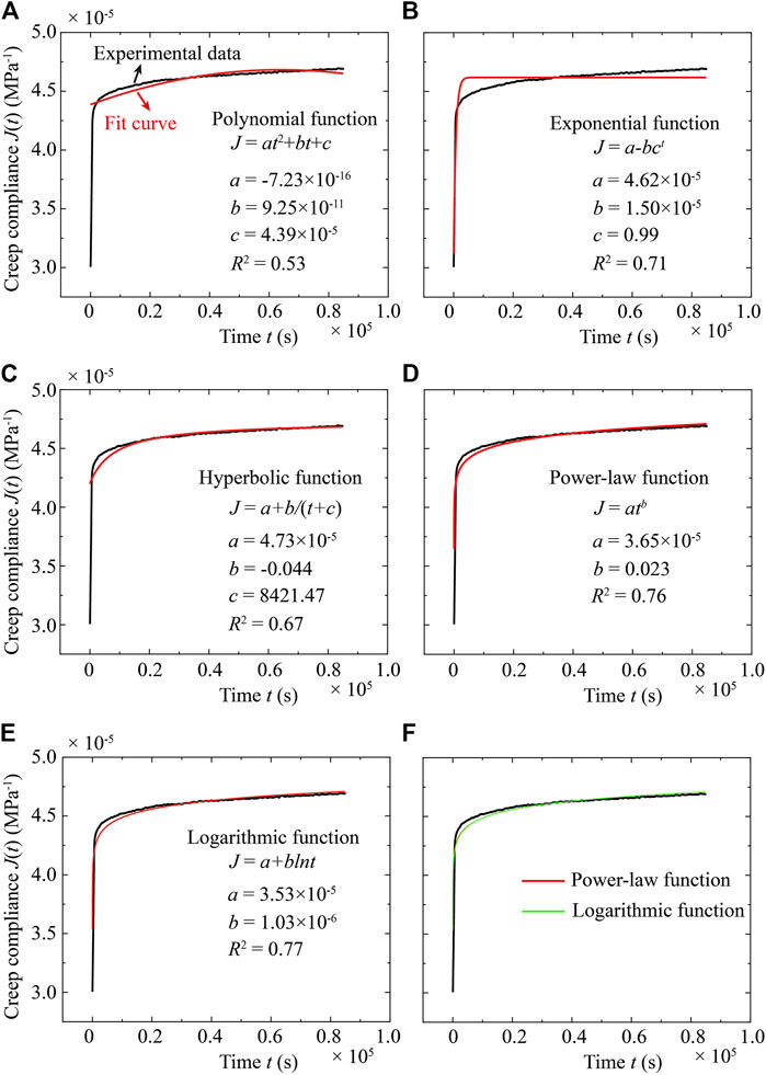
FIGURE B1. Comparison of different functions fit to the creep experimental data: (A) Polynomial function with three parameters; (B) Exponential function with three parameters; (C) Hyperbolic function with three parameters; (D) Power-law function with two parameters; (E) Logarithmic function with two parameters; (F) Comparison between the power-law and logarithmic functions. The experimental data are from the differential stress (60 MPa) stage of Sample S2.
Keywords: Wufeng-Longmaxi shale, creep, viscoplasticity, stress relaxation, in situ state of stress, shale gas reservoir
Citation: Cheng W, Zhang X, Jin J, Liu J, Jiang W, Zhang G, Zhang S and Ma X (2023) Time-dependent deformation of Wufeng-Longmaxi shale and its implications on the in situ state of stress. Front. Earth Sci. 10:1033407. doi: 10.3389/feart.2022.1033407
Received: 31 August 2022; Accepted: 16 November 2022;
Published: 13 January 2023.
Edited by:
Jingshou Liu, China University of Geosciences Wuhan, ChinaReviewed by:
Rui Liu, Southwest Petroleum University, ChinaZaobao Liu, Northeastern University, China
Copyright © 2023 Cheng, Zhang, Jin, Liu, Jiang, Zhang, Zhang and Ma. This is an open-access article distributed under the terms of the Creative Commons Attribution License (CC BY). The use, distribution or reproduction in other forums is permitted, provided the original author(s) and the copyright owner(s) are credited and that the original publication in this journal is cited, in accordance with accepted academic practice. No use, distribution or reproduction is permitted which does not comply with these terms.
*Correspondence: Jiandong Liu, bGl1amlhbmRvbmdAcGV0cm9jaGluYS5jb20uY24=; Shihuai Zhang, emhhbmdzaGlAZXRoei5jaA==, c2hpaHVhaXpoYW5nLnhoMUBnbWFpbC5jb20=