Study of the spectral characters–chlorophyll inversion model of Sabina vulgaris in the Mu Us Sandy Land

As the dominant shrub community plant in the Mu Us Sandy Land, S. vulgaris is the key factor of ecological environment restoration in the Mu Us Sandy Land, It is of great significance to explore the estimation and inversion of content based on spectrum for ecological environment evaluation and intervention in Mu Us Sandy Land. The SVC HR-1024 portable feature spectrometer and SPAD 502 chlorophyll meter were used to study Mu Us Sandy Land of S. vulgaris. The best band is screened by correlation matrix method, the best vegetation index is screened by Structural Equation Modeling model, and then the best inversion model is established by different mathematical modeling methods. Results revealed that the vegetation indices and chlorophyll content were correlated, combining the six vegetation indices revealed that 610–690nm and 700–940 nm were the bands with the highest correlation. In the selection of optimal vegetation index, NDVI, ratio vegetation index and mNDVI perform best and are suitable for subsequent modeling. Of the four models, the partial least squares model had the best fitting effect (R² > 0.91). The univariate linear regression model had the simplest processing procedure, but its accuracy was unstable (R² = 0.1–0.9). multivariate stepwise regression accuracy is also appropriate (R² > 0.8). The stability of BP neural network modeling is not high. Compare the four methods, PLS and multivariate stepwise regression have their own advantages, and the accuracy is higher, you can make a choice according to the demand as the late modeling method.

Introduction

The Mu Us Sandy Land is located in the southeast of the Ordos Plateau (Cheng et al., 2021), desertification in the region has become increasingly serious in recent decades due to the dramatic increase in human activities and the effects of climate change. Plants are important factors of ecological environment restoration in sandy land, how to better monitor plant growth, thus, effective and timely intervention before plant degradation is the key to current research on sandy plants. The dynamic changes of chlorophyll content of plant leaves are an important indicator of plant growth status and nutrient status (Liang et al., 2016; Shuang et al., 2021), therefore, monitoring and estimating the chlorophyll content of plants are now the focus of vegetation monitoring studies. Spectral monitoring technology in recent years because of its fast and non-destructive characteristics, It has become an important tool to analyze the estimation and inversion of chlorophyll content (Tong et al., 2020), vegetation water content (Yan et al., 2022), soil physicochemical properties (Pinheiro et al., 2017) and biomass (Zheng et al., 2019) etc. These results have efficiently deciphered the spectral characteristics of plants and their unique patterns, providing a theoretical basis for subsequent remote sensing monitoring and plant management.

Vegetation index has been one of the most effective, simple and commonly used methods to characterize vegetation. It is one of the research hotspots to establish a model combining chlorophyll and vegetation index to quantitatively estimate vegetation chlorophyll content. The model using the first derivative of the spectrum and chlorophyll has the ability of quantitative inversion of plant growth parameters, This method can effectively overcome the drawbacks brought by remote sensing technology, such as low resolution, climatic conditions at the time of image capture, time period, etc (Cao et al., 2017). Zhang et al. established the model of winter wheat chlorophyll by using the vegetation index randomly combined with the original spectrum and the first-order differential, the results showed that one session of differencing enhanced the correlation between vegetation index and winter wheat chlorophyll, meanwhile, the monitoring of vegetation index is better than the original spectrum, It shows the importance of suitable vegetation indices for green crop monitoring (Zhang et al., 2022). Sun et al. compared the correlation between the original band spectrum, first-order differential spectrum, vegetation index and wavelet coefficient and maize canopy chlorophyll, results also showed that the highest accuracy was achieved with the model built with vegetation index, followed by the model built with first-order differentiation, both with R² > 0.6 (Sun et al., 2022). Some scholars also mainly compare different vegetation index, but different plants or crops do not have the same sensitivity to different vegetation index (Miao and Zhang, 2018; Zhang et al., 2018). The current research progress can be seen that the technique of hyperspectral inversion chlorophyll model is relatively mature, among them, one-dimensional linear and multiple linear regression models have been widely used to construct the relationship between spectral characteristics and chlorophyll content, and generally the R² can reach above 0.8 (Atherton et al., 2016; Sun, 2019). With the development of science and technology, many scholars have tried to use the machine algorithm of big data platform for chlorophyll inversion, but the variation and uncertainty of the input parameters can affect the accuracy of the model, also this algorithm is not applicable to all vegetation types (Li et al., 2016). Some scholars also use physical model to invert chlorophyll, but the algorithm of physical model is complicated, the process of inputting variables contains more uncertainties, and the accuracy is not improved much, so physical models are not suitable for general use (Mahmoud and Done, 2018). All three compared, the linear regression modeling based on two or more bands is more sensitive in terms of the information characterized than the single band, It can also eliminate to a certain extent the problem of overfitting of bands caused by too many multi-bands (Shuang et al., 2021). Tong et al. showed that although the rich spectral information can provide various information on vegetation in more detail, too detailed band information will bring some interference to the inversion model (Tong et al., 2016). Ke et al. used statistical models, physical models, and a mixture of both models to estimate the leaf area of crops, The results showed that high correlation bands could enhance the sensitivity of the model to LAI, but the low correlation band will reduce the accuracy of the model (Ke et al., 2016). Therefore, the selection of characterization sensitive bands and vegetation index is important for the improvement of model accuracy. At present, choosing the best band or choosing the high correlation coefficient are the two methods commonly used. However, the method of selecting the best band only considers a single relationship between chlorophyll and spectrum, and the indirect effects of other values will be ignored. And while the selection of the best index method is highly accurate, more problems can be considered in band combination, but there is no guarantee that all vegetation indices and chlorophyll will have the greatest correlation. Therefore, Cheng et al. combined the two methods with the proposed optimal index-correlation coefficient method, spectral data and chlorophyll content of winter wheat was analyzed and the three most sensitive bands were finally extracted. It is also proved that the optimal index-correlation coefficient is more accurate than the single method (R² = 0.83) (Cheng et al., 2015). But the disadvantage of this approach is that it is impossible to assess the importance of each variable in the process. Chen et al. combined the RF algorithm with K proximity regression and their model was more reliable in predicting the LAI of maize (Chen et al., 2020). Thus, in the current inversion model for vegetation spectra and other eigenvalues, it is mainly used for the screening of bands, improvement of accuracy needs further verification. There is still great research space for selecting the best band and the best vegetation index.

In summary, most of the current studies on spectral-chlorophyll inversion models have focused on agricultural crops, and fewer studies have applied such studies to the inversion of sandy vegetation. Structural Equation Modeling (SEM) allows for the simultaneous measurement of observed variables, latent variables, and the influence relationships and pathways between each variable (Li et al., 2022). There are also few studies that use SEM to extract optimal vegetation index, therefore this study attempts to select the optimal vegetation index using structural equation modeling, selecting the best band by correlation matrix method, chlorophyll prediction model using the best vegetation index and the best band selected by the two. In order to realize high precision spectral - chlorophyll inversion of S. vulgaris in Mu Us Sandy Land, provide theoretical basis for regional desertification land management and restoration of degraded ecological environment.

Methods

Study area

The Mu Us Sandy Land (37°27’−39°22’N, 107°20’–111°50’E) (Guo et al., 2021) has a total area of 4 × 104 km². The midwestern part is a wavy plateau with the highest altitude (1,600 m) (Karnieli et al., 2014). Dunes of various types account for 77% of the total area and mobile dunes account for 47% (Liang and Yang, 2016). The annual rainfall fluctuates greatly, increasing from 250 to 440 mm from the northwest to southeast. Most of the precipitation is concentrated to the summer and the intensity of precipitation is the highest in August, which usually lasts for several days and up to >10 days. Therefore, drought and flood disasters easily occur, of which drought is more frequent (Zhou et al., 2020). The annual average temperature ranges from 6.0 to 9.0°C (7.6°C average), the average temperature in January ranges from (−) 8.7°C to 12°C, and the average temperature in July ranges from 20°C to 24°C. The potential evaporation ranges from 2100 to 2500 mm. The main soil type is chestnut soil, which is alkaline and lacks organic matter and nutrients. The northwest consists of desert steppe, which changes from steppe to forest-steppe in the southeast. Grasslands account for 90% of the total area. Most of the vegetation grows on sandy girders. The vegetation types include sandy, meadow, halophytic, and marsh vegetation, of which sandy vegetation accompany all types of sandy land and has the largest area (Han et al., 2020).

Acquisition of spectral data

Spectral data were measured using SVC HR-1024 portable ground object spectrometer (Spectra Vista, USA). The spectral range was 350–2,500 nm, the number of channels was 1,024, and the spectral resolution was ≤3.5 nm within 350–1000 nm, ≤8.5 nm within 1000–1850 nm, and ≤6.5 nm within 1850–2500 nm. The minimum integration time was 1 ms and the signal acquisition method was Bluetooth transmission (Yang and Li, 2014).

Field measurements of the plant spectrum were greatly affected by the solar altitude angle (clear and cloudless weather should be selected for measurement). The measurement time ranged from 10:00 to 14:00 (Niu Y. L. et al., 2017). Spectral measurements of ground objects in the study area were carried out in early May and mid-July 2019. Dark current collection and whiteboard calibration were required before measurement. In the event of obvious weather changes, such as strong wind, it was necessary to calibrate again with a whiteboard and every time the location changed. To ensure the accuracy of the test results, samples were randomly collected. A total of 70 groups were measured with 5 replicates per group (350 total). A group of samples is: The spectrometer measures the same location of a plant five times at the same time, that is, the spectrometer probe does not do anything at the same location of the plant, but the measurement is repeated five times (Although they are in the same position, the five data are different because the reflection of the spectrum and the change of the environment will affect the measurement results). Five repetitions were used for subsequent spectral data fusion. Among them, originally decided to choose the 55 groups were used for the model establishment and 15 groups were used for model verification. But since the final data has outliers, after eliminating four sets of data and considering the accuracy of the modeling set and the validation set, it was finally decided that 46 sets would be used for modeling and 20 sets for validation. For the measurements, the measurement time of each spectral datapoint was 5 s and the measurement height was 50 cm from the probe to the ground object. The sampling points in the study area are shown in Figure 1. The top view of spectral data acquisition is shown in Figure 2A. The monitoring range of the spectrometer probe is presented in Figure 2B. The identification of S. vulgaris refers to “flora of China” and “Chinese Virtual Herbarium.” The number of S. vulgaris is LZD0000136.

FIGURE 1

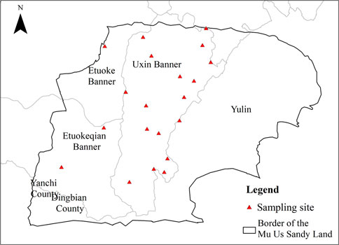
FIGURE 1. Distribution of major specimens and sample plots in the Mu Us Sandy Land.

FIGURE 2

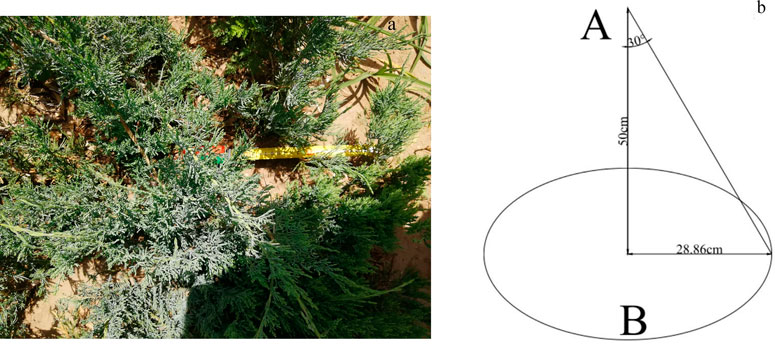
FIGURE 2. Top view of the measured spectral data (A). Schematic diagram of the spectral data and chlorophyll content measurements (B). Position A is the probe position of the spectrometer. Elliptical area B is the area that was monitored by the probe. The probe was 50 cm away from the S. vulgaris canopy. When measuring the chlorophyll content, it was within the range monitored by the probe. The radius of the chlorophyll monitoring area was 28.86 cm.

Determination of the chlorophyll content

The chlorophyll content was measured using a Soil Plant Analysis Development Unit (SPAD) 502 chlorophyll meter (Konica Minolta, Japan). The SPAD-502 chlorophyll meter does not damage plants. During the spectral measurements, the selected plants were measured in an area with a diameter of 22 cm around the center of S. vulgaris. We took a total of 560 measurements. The chlorophyll content was measured 8 times in each plot. The average value was used as the chlorophyll SPAD value corresponding to the spectral data.

Fusion of the spectral data

First, the SVC HR-1024 software of the ground object spectrometer was used to eliminate bands with large variations within the spectral curve data. A normal spectral curve has no intersection and is smooth. Then, the SIG File Overlap/Matching function was used to match the data. Finally, the SIG File Merge function was used to merge the data and output the data into Excel format. As already shown above, the same plant will be measured 5 times, 5 times is a set of data, 5 times is actually a representative of the state of a plant, so 5 times repeated measurement is to reduce the measurement error, and the fusion process of spectral data is to fuse this set of (5 times) data through the software (SVC-HR1024) that comes with the spectrometer through the professionally set steps to 5 groups of data accuracy and fuse them into one set of data. The fusion process of 5 sets of data is the same as taking the average, but the fusion process is carried out under the software’s own function, which improves the accuracy and efficiency of the data.

Smoothing of the spectral data

Due to differences in band responses to the energy during the spectral data measurements, the spectral curves always had noise, so the data curves needed to be smoothed to eliminate the small amount of noise contained in the signals. Common smoothing methods include the moving and static average methods. The moving average method includes three-point, five-point, and nine-point smoothing methods. The five-point smoothing method was used in this study (Yang and Li, 2014). A comparison of before and after smoothing is shown in Figure 3.

FIGURE 3

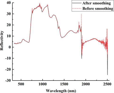
FIGURE 3. Comparison of the spectral smoothing effect before and after smoothing. The red dotted line is before smoothing and the black solid line is after smoothing. The impact of noise in the 1800–2500-nm band was obvious. After smoothing, the noise error was reduced and the accuracy of the data was enhanced.

Resampling of the spectral data

Resampling of the spectral data was conducted to ensure the accuracy of the spectral data prediction model established in the later stage (Niu Y. et al., 2017). ENVI 5.1 (Exelis Visual Information Solutions USA) was used to resample the spectral data. The resampling interval was 10 nm.

First-order differential processing

First-order differential processing of the spectral data eliminates the systematic error of different data, better eliminates the effects of noise on the data, and results in more prominent spectral vegetation characteristics. The data after first-order differential processing were calculated as follows (Wang et al., 2017) (Figure 4), the first-order differential equation is shown in Table 1:

$R\left({\lambda }_i\right)=\frac{\left[R\left({\lambda }_{i+1}\right)-R\left({\lambda }_i\right)\right]}{\Delta {\lambda }_i}\times R,(1)$

where R (λ_i) is the first-order differential spectrum of wavelengths λ_i + ₁, λ_i, R (λ_i) and R (λ_i + ₁) are the original spectral reflectance at I and I + 1, and Δ(λ_i) is the wavelength difference between λ_i + ₁ and λ_i.

FIGURE 4

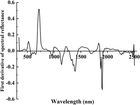
FIGURE 4. Spectral data after first-order differential processing strengthened the change of the absorption valley or reflection peak at each place.

TABLE 1

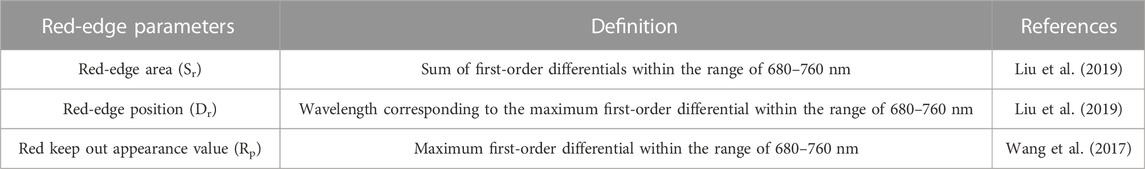
TABLE 1. Red-edge parameters.

Statistical analysis and modeling

Selection of the vegetation index

The correlation between the spectral data and chlorophyll content was analyzed using MATLAB R2012a (MathWorks USA). The selected vegetation indices and calculation formulas are shown in Table 2. The original spectral band is used to calculate for the subsequent selection of the optimal band, and then the selection of a more appropriate vegetation index to prepare.

TABLE 2

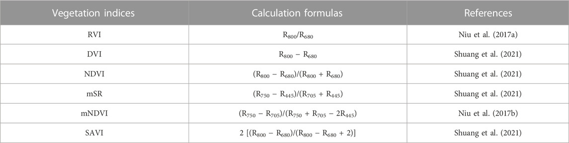
TABLE 2. Vegetation indices and their respective calculation formulas.

Extraction of the optimal spectral index wavelength combination

The original spectral data of the 350–2500-nm band were selected. The reflectance of any composition was analyzed using the normalized vegetation index (NDVI), ratio vegetation index (RVI), and difference vegetation index (DVI), modified simple ratio (mSR), modified normalized vegetation index (mNDVI), soil–adjusted vegetation index (SAVI) The correlation between the chlorophyll content and reflectance was analyzed using MATLAB R2012a. The formulas are as follows (Chuvieco, 2016):

$N_I\left(R_{{\lambda }_1},R_{{\lambda }_2}\right)=\left|R_{{\lambda }_1}-R_{{\lambda }_2}\right|/\left|R_{{\lambda }_1}+R_{{\lambda }_2}\right|,(2)$

$R_I\left(R_{{\lambda }_1},R_{{\lambda }_2}\right)=R_{{\lambda }_1}/R_{{\lambda }_2},(3)$

$D_I\left(R_{{\lambda }_1},R_{{\lambda }_2}\right)=R_{{\lambda }_1}-R_{{\lambda }_2}.(4)$

Mathematical modeling

The prediction model of the chlorophyll content was established using unary linear regression, multiple stepwise linear regression, the partial least squares method and BP neural network. The unitary linear regression model has small input and output, and the calculation method is convenient and simple, which was completed using Origin 2017 (Liu and Yang, 2020). The multiple stepwise linear regression model selects one of the most important independent variables in the regression equation based on the weight of each datapoint involved in modeling. It is widely used in spectral prediction modeling and was completed using SPSS 26 (Liu and Yang, 2020). The partial least squares method is widely used in the field of spectroscopy. Through the analysis of multiple independent and dependent variables, their correlation can be maximized in the modeling process, which was completed using MATLAB R2012a. The advantages of PLSR: It is a combination of correlation analysis, principal component analysis and multiple linear regression analysis. It can reduce the dimension of high spectral data and use effective data for modeling. PLSR will also consider the extraction of principal components from independent variables and dependent variables during modeling, so that the modeling accuracy is higher. BP neural network consisting of three input layers and one output layer was constructed for training, the number of iterations is 12, the learning accuracy is 0.01, and the training target is less than 0.001 root mean square error. BP neural network modeling by writing program code in MATLAB R2012a software. To verify and increase the accuracy of the model, 66 groups of data were separated into 46 groups used for the prediction model data and 20 groups used for the validation model data.

Evaluation of the accuracy of the hyperspectral prediction model was based on the determination coefficient and total root means square difference. R² is related to the stability of the model; as the R² value increases, so does the stability of the model. Moreover, R_MSE is related to the prediction ability of the model; the smaller the R_MSE value is, the higher the accuracy of the established model and the stronger the prediction ability are (Sun 2017).

Extraction of the optimal vegetation index from the structural equation model

The structural equation model was developed from a linear equation. Its uses the Bayesian estimation method to hypothetically guess the data and various indicators through the previous empirical theory, and extracts the relationship between unmeasurable information from the measured information. Based on the previous retrieval, the structural equation was used to estimate and test the relationship between non-directly measurable variables in psychology, management, and economics (Hekmati et al., 2020).

The structural equation model was used to screen the vegetation indices. Different vegetation indices represent different vegetative chlorophyll and spectra. For example, the NDVI overcomes disadvantages of the RVI, limits the value to [−1, 1], and eliminates most changes in the irradiance conditions related to solar angle, terrain, cloud shadow, and atmospheric conditions. However, in areas with dense vegetation, the NDVI tends to supersaturate early and does not timely reflect the growth process from yellow to dry during vegetative growth (Sharafatmandrad and Mashizi, 2020). Therefore, the vegetation index selected for the final model greatly affects the accuracy of the model.

In this study, based on the six vegetation indices used for establishing linear regression model and BP neural network, the three vegetation indices with the highest correlation and the red edge parameters were selected to build SEM, and the lower accuracy was used to verify the stability of the high correlation of the selected vegetation indices. Then multiple regression, PLSR and BP neural network were built with highly correlated vegetation indices.

Results

Chlorophyll content statistics of S. vulgaris

As can be seen from Figure 5, the average value of chlorophyll content in the total sample set was 7.96, and the mean value of chlorophyll content in the modeling set was 7.88, 0.08 lower than the total sample average. The mean value of the validation set is 8.28, that’s 0.32 higher than the total sample average. The total sample means are below the median, and the three coefficients of variation of 9.10%, 9.27%, and 8.92% are less than 10%, and the data variability is smaller.

FIGURE 5

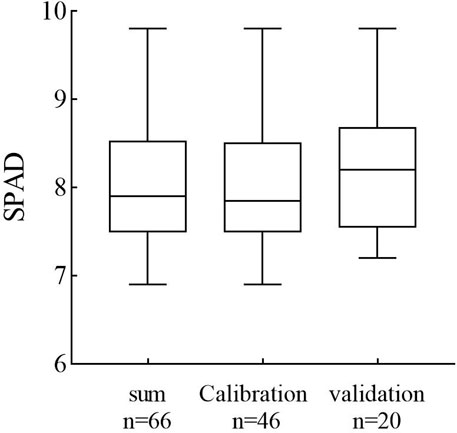
FIGURE 5. Boxplots of Chlorophyll content of S. vulgaris, lower and upper box boundaries represent the quartiles (25% and 75% quantiles, respectively), the whisker is min-max, and the solid lines across each box are the median.

Analysis of the spectral characteristics and chlorophyll content of S. vulgaris

Spectral characteristics of S. vulgaris at different periods (Figure 6). Green plants contain various pigments (e.g., chlorophyll, lutein, and carotenoids) in their leaves within the visible light band, of which, chlorophyll plays the most important role (Tang et al., 2004). Due to the strong absorption of electromagnetic waves and other radiation within this band, the reflection and transmission of leaves are very low. In the 420–450-nm blue waveband and 620–780-nm red waveband, chlorophyll strongly absorbs radiation waves and easily forms absorption valleys. The reflection between these two absorption valleys is reduced and forms reflection peaks, which makes plants appear green. If normal plant growth is inhibited in the visible band, a decrease in the chlorophyll content will increase the reflection of plants within the blue-green band and reduce absorption.

FIGURE 6

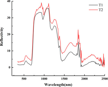
FIGURE 6. The spectral curves of S. vulgaris represent the law of “five grains and four peaks.” There is some difference in reflectance, but the difference is not significant.

The curve obviously showed characteristics of the “five grains and four peaks” of green plants. The main characteristics of the vegetation spectrum are “red valley” and “green peak” within the visible light band. The red-edge appears between 680–760 nm, which is a diagnostic spectral feature of vegetation and the red valley forms high reflection in this band. There is a small reflection peak near the “green peak” wavelength at 800 nm. As the chlorophyll content increases, the spectral curve will shift to the right.

Within the near-infrared band, the main influencing factor of green plants is the cell structure inside the leaves. In this band, the absorption energy of the leaves is low and the reflection and transmission are similar. High reflection is formed around 680–1300 nm.

Within the infrared band, the transmission of plants is small and the absorption and incidence are similar. The main influencing factor is the water content in plant cells. Generally, two main water absorption bands are formed around 1400 and 1900 nm.

Correlation of two-band raw spectral indices with chlorophyll of S. vulgaris

In the correlation analysis between the ratio of the original spectral reflectance of the two bands, vegetation indices, and the improved RVI, DVI, NDVI, mSR, mNDVI and SAVI with chlorophyll (Figure 7). With regard to the RVI, the highest correlation was detected between the combined bands of 610–680 nm and 700–940 nm. With regard the DVI, the highest correlation was between the combined bands of 350–430 nm and 650–690 nm. For the NDVI, the highest correlation was between the combined bands of 470–500 nm, 610–680 nm, and 740–840 nm, the highest correlation of mSR was found in the combined bands of 790–930 nm and 600–620 nm. The highest correlation of mNDVI is found in the combined bands of 780–1180 nm and 1410–1790 nm, the highest correlation of SAVI is found in the combined bands of 2020–2080 nm and 2280–2310 nm. Through the comparative analysis, we found that the bands with the highest correlation between the NDVI and chlorophyll content were 660 and 790 nm, the RVI was best at 630 and 720 nm, and the DVI was 360 and 450 nm, the best mSR performance is 570 and 890 nm, the best mNDVI performance is 1100 and 1,500 nm and the best performing SAVI was 2290 and 2050 nm. Therefore, in follow-up monitoring, we focused on the bands with better performance to monitor S. vulgaris growth.

FIGURE 7

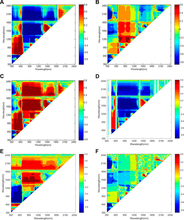
FIGURE 7. Correlation analysis of the original band spectrum and chlorophyll content: RVI (A), DVI (B), NDVI (C), mSR (D), mNDVI (E), SAVI (F). Blue indicates high negative correlation and red indicates high positive correlation.

Selection of the optimal index

To screen the vegetation index, firstly, all six vegetation indicators selected in Table 2: RVI, DVI, NDVI, SAVI, mSR and mNDVI were used for modeling with chlorophyll (Figure 8A), by building this model, it was found that among them, mNDVI, RVI and NDVI had the highest correlation with chlorophyll, their correlations were all greater than or equal to 0.65 and significantly correlated. While the correlations between DVI, SAVI and chlorophyll were <0.5 and none of them were significant, mSR is a negative correlation.

FIGURE 8

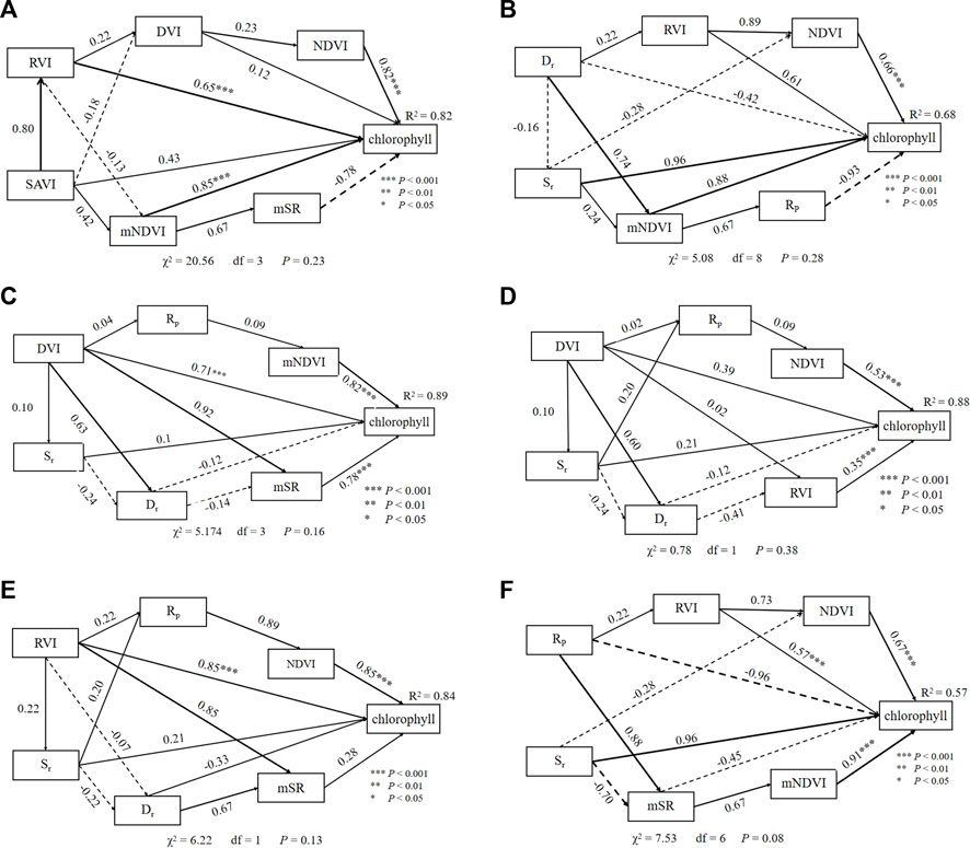
FIGURE 8. Analysis of the relationship between the chlorophyll content and the NDVI, RVI, DVI, mSR, mNDVI, SAVI, red-edge amplitude, red-edge area, and red-edge position using the structural equation model. The solid and dotted lines represent positive and negative coefficients, respectively. The thickness of the arrows indicates the size of the standardized path coefficient. R² represents the proportion of variance interpretation of each endogenous variable. (A) is the screening vegetation index, (B) is the high correlation vegetation index with red edge parameter, (C), (D), (E) and (F) are to verify the correlation between vegetation index and red edge parameters.

The high correlation vegetation index selected in the previous step were then combined with the red-edge parameters to build the second SEM (Figure 8B), and it was found that the index with high correlation between red-edge parameters and chlorophyll were S_r and R_P, the correlation coefficient of S_r was as high as 0.96 and R_P also reached 0.93, but R_P was negatively correlated with chlorophyll.

In order to verify the accuracy of the selected high correlation indicators, six vegetation indexes were selected to establish SEM (Figures 8C–F), which inevitably included the screened high correlation indicators, namely mNDVI, RVI, NDVI and S_r, the rest were selected by the correlation size established in the two models (Figures 8A,B). Finally, it was found that the characterization of mNDVI, RVI and NDVI was always relatively stable, but S_r and R_P of the red-edge parameters were not stable, sometimes with correlation <0.5, the correlation with chlorophyll was high and low in different combinations. It shows that its correlation with chlorophyll is more easily affected by other factors. Therefore mNDVI, RVI and NDVI are best suited for subsequent modeling applications, and the red edge parameters are to be further verified for accuracy in modeling.

Optimization of chlorophyll inversion models of S. vulgaris

Univariate linear regression model

The univariate linear regression analysis was conducted on the spectral data and chlorophyll content (Figure 9). Results revealed that the SAVI had the best fitting effect (R² = 0.9), the second is NDVI, which R² = 0.89.

FIGURE 9

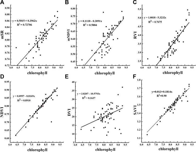
FIGURE 9. Univariate linear regression analysis fitting the chlorophyll content and the mSR (A), mNDVI (B), RVI (C), NDVI (D), DVI (E), SAVI (F).

With the exception of the DVI, the correlation between other vegetation indices and the chlorophyll content are greater than 0.5, in which, the R² values of the mSR and RVI were >0.7; the applicable condition of the RVI is considered to be “the ratio of scattering of green leaves in the near-infrared band to chlorophyll absorption in the red band.” (Tulokhonov et al., 2014). The RVI is more suitable for studying the spectrum of green plants; therefore, the effect is ideal when used for the correlation between the green plant spectrum and chlorophyll content. Similarly, the mSR corrects the specular reflection efficiency of the leaves. Thus, the fitting effect of the mSR in this study was ideal. Although the mNDVI is an improved value of the NDVI, it is sensitive to small changes in the leaf canopy, gap segments, and senescence (Malingreau, 1989). In previous studies, it was mostly used for fine agriculture, vegetation monitoring, and vegetation stress detection. The mNDVI was selected as it is suitable for vegetation monitoring. However, according to the linear fitting results, the measurements used for S. vulgaris monitoring were not ideal. The mNDVI should be used for spectral monitoring broad-leaved tree species or monitoring areas with high vegetation coverage. Therefore, from the results of the one-dimensional linear regression model, the modeled vegetation index should be chosen SAVI and NDVI.

Multiple stepwise regression model

An advantage of the multiple stepwise regression analysis is that the regression equation includes all independent variables that have a significant effect on the dependent variables; The red edge parameter and vegetation index were established separately in this model, and both of them had three variables. However, the reason why multiple stepwise regression only showed the first two variables was that: when p>0.05, the independent variable had no statistical significance in this model, and correspond variables should be deleted in the regression model. When p<0.05, this variable is statistically significant in the model and should be retained. It does not include the regression equation of independent variables that have no significant effect on the dependent variables. Stepwise regression analysis is based on this principle. Its essence is to derive an algorithm for studying and establishing the optimal multiple linear regression equation based on multiple linear regression analysis. It also uses the principle of regression analysis, adopts the double test principle, and gradually introduces and eliminates independent variables to establish the optimal regression equation (Wang et al., 2015).

In this study, the vegetation indices and red-edge parameters were used as independent variables and the chlorophyll content as the dependent variable. Two multivariate linear stepwise regression models were established and the regression equation was constructed (Table 3). The fitting degree of the model constructed by the vegetation indices was much higher than the model constructed by the red-edge parameters. Its R_MSE was also relatively small, thus, the accuracy of the prediction model was high. Generally speaking, the accuracy of the multivariate stepwise regression model was higher than the univariate linear regression model.

TABLE 3

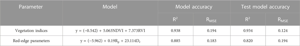
TABLE 3. Multiple stepwise regression model equation.

Partial least squares regression model

The partial least squares regression models of different leaf coverage areas were established. We used the vegetation indices and red-edge parameters as inputs. For better accuracy of the results, three indices, the mNDVI, RVI, and NDVI, which had the best characterization of the chlorophyll content, were selected to establish the partial least squares regression model; the three vegetation indices and red-edge parameters were used as inputs (Table 4). Compared to the multiple stepwise regression model, the partial least squares regression model had higher accuracy, the correlation coefficients of the vegetation indices and red-edge parameters models increased, and R_MSE decreased to <0.1. The fitting effect of the model using the vegetation indices as the inputs was higher than the red-edge parameters.

TABLE 4

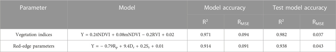
TABLE 4. Partial least squares regression equation.

Based on three regression modeling methods, the model accuracy established by the partial least square method was better than the univariate linear regression model and multivariate linear regression model, and its fitting effect was the best.

BP neural network analysis

Table 5 lists the BP neural network models constructed based on the three spectral parameters, with the three spectral parameters (NDVI, mNDVI, and RVI) as the input layer of the model and chlorophyll content as the output layer, optimal accuracy after multiple training implicit layers. The coefficient of determination R² is 0.96 and R_MSE is 0.08, the accuracy of the model is high. By comparing the regression models, it can be seen that the model established by BP neural network has higher accuracy. The fitted lines of predicted and actual values are shown in Figure 10.

TABLE 5

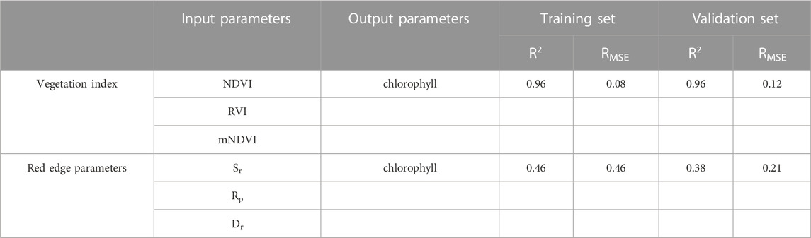
TABLE 5. BP neural network modeling parameters and results.

FIGURE 10

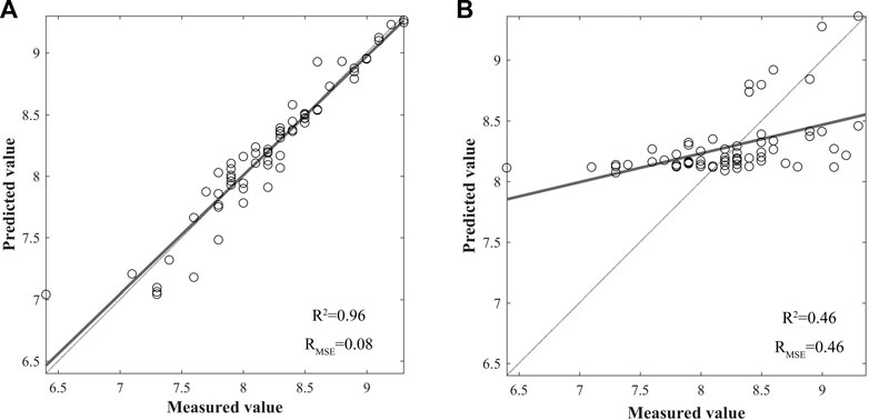
FIGURE 10. Prediction results of SPAD values of chlorophyll spectral reflectance BP neural network model test set. BP neural network model based on vegetation index (A), BP neural network model based on red-edge parameters (B).

To determine the accuracy of our filtered optimal vegetation index, a BP neural network model was established for the red-edge parameters. Three red-edge parameters (S_r, R_p, D_r) were used as the input layer and chlorophyll content as the output layer, optimal accuracy after multiple training implicit layers. From the results of the modeling, its coefficient of determination R² is 0.46 and R_MSE is 0.46, the model accuracy is low. The regression model is more accurate than the BP neural network in the model built with red-edge parameters.

Discussion

As a sand-fixing form of vegetation found in fixed and semi-fixed sandy land, S. vulgaris plays an important role in preventing wind, fixing sand, and improving the ecological environment. In this study, we used S. vulgaris obtained from the Mu Us Sandy Land as the research object. The spectral data and chlorophyll content of S. vulgaris were measured. Compared to ordinary broad-leaf trees, the chlorophyll content of S. vulgaris was generally low. This may be because the leaf type of S. vulgaris is coniferous and the measurement principle of the chlorophyll meter is more suitable for broad-leaf trees (Ates and Kaya, 2021). Even when leaves were covered in small holes, there were some gaps or the leaves artificially integrated into a cluster. Under these conditions, the instrument will have measurement or data error because the leaves are too thick. Therefore, the spectrophotometer method will continue to be used to measure the chlorophyll content in subsequent experiments.

In this study, four modeling methods were used to predict the chlorophyll content of S. vulgaris and the model verification results were ideal. The modeling results showed that the modeling methods feasibly predicted the chlorophyll content of S. vulgaris and monitored its growth by using spectral characteristic parameters. The univariate linear fitting effect was unstable, as it depends on the selection of a vegetation index and different plants are sensitive to different vegetation indices (Gao et al., 2020); hence, the univariate linear fitting is not recommended. The fitting effects of the multiple stepwise regression and partial least squares methods were good (Hair et al., 2012), the stability of the BP neural network modeling results is not high, which is highly dependent on the vegetation input layer selected.; thus, it is more appropriate to select the multiple stepwise regression and PLS method for modeling, BP neural network modeling as a vegetation index as an input layer is more appropriate.

Among the four methods, the red-edge parameters were extracted using the first-order differential of the original spectral data. Although the data processed by the first-order differential can better reduce human interference and strengthen its absorption effect on water (Zhu et al., 2020; Sun et al., 2021), this study focused on the modeling of the visible light band and chlorophyll content. Therefore, the accuracy of the model established by the vegetation index was higher than the model established by the red-edge parameters, was more stable, and universally applicable for the model established with the chlorophyll content.

In previous studies on plant hyperspectral characteristics and chlorophyll, in the models established by the spectral characteristics of plants and different chlorophyll contents, the value of the determination coefficient reached >0.8, which indicated that good correlation can be attained between the spectral characteristics of green plants and chlorophyll through the analysis of vegetation indices (Dzikiti et al., 2010; Xu et al., 2019; Sun et al., 2021). The significance of this correlation lies within an inversion model of green plant growth, which can be established using changes in the plant chlorophyll content. Through the analysis of model data, any change in green plants during the growth process can be determined, achieving the timely prevention and control of diseases and pests, and human regulation.

Due to differences in the growth environment and internal factors, the spectral reflectance curves of different vegetation types are not the same, but they are found in the form of “five grains and four peaks.” Therefore, this study is applicable to other vegetation types in addition to S. vulgaris. The extraction of vegetation indices from the original spectral reflectance of vegetation is helpful for highlighting the spectral characteristics of vegetation and establishing a model. When the operation mode and measurement conditions change, the wavelength of the preferred vegetation index also changes. Therefore, this study used the structural program model to optimize the best vegetation index for subsequent modeling.

In previous studies, the structural equation model has been primarily used to study deep-seated correlations between dependent and independent variables. However, the structural equation model can mine deep-seated correlations, the structural equation model is more complex in terms of modeling and analysis. The purpose of this study was to construct a model with a good fitting effect between the spectral data and chlorophyll content, and relatively good operation. Therefore, the structural equation model was not used to model mathematical in this study. However, based on the advantages of the structural equation model, selection of the optimal index for mining is appropriate. Moreover, the mNDVI, RVI, and NDVI indices were compared and screened out by the structural equation model with the unselected vegetation indices, the mNDVI and mSR. The results revealed that the screened mNDVI had higher accuracy, and the RVI and NDVI indicated that it was feasible to screen indices with higher accuracy by using the structural equation model. Because the spectral characteristics of S. vulgaris are the same as general green plants, the findings of this paper are applicable to other desert plants.

Conclusion

In this paper, the spectral reflectance and chlorophyll content of S. vulgaris were measured using an SVC HR-1024 portable ground object spectrometer and SPAD502 chlorophyll meter. The data were post-processed using MATLAB R2012a, SPSS26, and other software. The ground object spectral characteristics, characteristics of the chlorophyll content, and the relationship between them were investigated. The results indicated the following:

1) The spectral curve of S. vulgaris had a reflection peak at 570 nm within the visible band, an absorption valley at 680 nm, and obvious reflection platform within the near-infrared band, which conforms to the spectral characteristics of green plants;

2) The vegetation indices and chlorophyll content were correlated in the original spectral composition of S. vulgaris. Combining the six vegetation indices revealed that 610–690nm and 700–940 nm were the bands with the highest correlation;

3) A certain correlation was detected between the vegetation indices, red-edge parameters, and chlorophyll content. The fitting effect of the model established by the vegetation index was better than the model established by the red-edge parameters. Screening vegetation indices with the SEM model showed that the highest correlation and the most stable performance were mNDVI, RVI and NDVI, and the R² in the characterization of red edge parameters with chlorophyll was not stable and therefore not suitable for subsequent modeling, and the most suitable indices for modeling were mNDVI, RVI and NDVI.

4) Among the four modeling methods, the PLSmodel had the highest accuracy (R² > 0.9) and was the most stable. The univariate linear regression model had the simplest processing procedure, but its accuracy was not high, although linear regression model had a great relationship with the selected vegetation indices. Results are sometimes not objective. The lowest R² was 0.16, while the greatest was0.90. The R² of the multiple linear regression model ranged from 0.88 to 0.94. The accuracy of the BP neural network established by the vegetation index is high, but the accuracy established by the red edge parameter is very low, indicating that the stability is not high. Compare the four methods, PLS and multivariate stepwise regression have their own advantages, and the accuracy is higher, you can make a choice according to the demand as the late modeling method.

Data availability statement

The original contributions presented in the study are included in the article/supplementary material, further inquiries can be directed to the corresponding author.

Author contributions

QL gave important suggestions for all the changes in the revised draft. NW wrote the main manuscript text and XH. prepared Figures 1–10. In addition, GY. reviewed and revised the manuscript. GJ, FL, H.C, XL, TZ, and XG Carried out field survey in Mu us Sandy land. All authors discussed the results and commented on the manuscript. The identification of Sabina vulgaris refer to 《flora of China》. The final determiner of the plant is the corresponding author GY. No samples were collected in this experiment, and the S. vulgar is in the study area was not damaged.

Funding

This research was supported by Inner Mongolia Autonomous Region’s major scientific and technological project “Research and Industrialization Demonstration of Near-Natural Restoration Technology of Sandy Ecosystem” (Grant No. 2019ZD003). This research was supported by Key technology research project of Inner Mongolia Autonomous Region Science and Technology Plan “Wise soil and water conservation technology in loess hills and gullies” (2021GG0070).

Acknowledgments

We thank LetPub (www.letpub.com) for its linguistic assistance during the preparation of this manuscript.

Conflict of interest

The authors declare that the research was conducted in the absence of any commercial or financial relationships that could be construed as a potential conflict of interest.

Publisher’s note

All claims expressed in this article are solely those of the authors and do not necessarily represent those of their affiliated organizations, or those of the publisher, the editors and the reviewers. Any product that may be evaluated in this article, or claim that may be made by its manufacturer, is not guaranteed or endorsed by the publisher.

References

Ates, F., and Kaya, O. (2021). The relationship between iron and nitrogen concentrations based on kjeldahl method and SPAD-502 readings in grapevine (Vitis vinifera L. cv.‘Sultana seedless’). Erwerbs-Obstbau 63 (1), 53–59. doi:10.1007/s10341-021-00580-8

CrossRef Full Text | Google Scholar

Atherton, J., Nichol, C. J., and Porcar-Castell, A. (2016). Using spectral chlorophyll fluorescence and the photochemical reflectance index to predict physiological dynamics. Remote Sens. Environ. 176, 17–30. doi:10.1016/j.rse.2015.12.036

CrossRef Full Text | Google Scholar

Cao, Q., Miao, Y., Li, F., Gao, X., Liu, B., Lu, D., et al. (2017). Developing a new Crop Circle active canopy sensor-based precision nitrogen management strategy for winter wheat in North China Plain. Precis. Agric. 18, 2–18. doi:10.1007/s11119-016-9456-7

CrossRef Full Text | Google Scholar

Chen, Z., Jia, K., Xiao, C., Wei, D., Zhao, X., Lan, J., et al. (2020). Leaf area index estimation algorithm for GF-5 hyperspectral data based on different feature selection and machine learning methods. Remote Sensing 12 (13), 2110.

CrossRef Full Text | Google Scholar

Cheng, Y., Zhang, J., Meng, P., Li, Y., Wang, H., Li, C., et al. (2015). Improvement of algorithm used for extraction hyperspectral feature bands of vegetation. Transactions of the Chinese Society of Agricultural Engineering 31 (12), 179–185.

Google Scholar

Cheng, Y., Yang, W., Zhan, H., Jiang, Q., Shi, M., Wang, Y., et al. (2021). On change of soil moisture distribution with vegetation reconstruction in Mu us sandy land of China, with newly designed lysimeter. Front. Plant Sci. 12, 609529. doi:10.3389/fpls.2021.609529

PubMed Abstract | CrossRef Full Text | Google Scholar

Chuvieco, E. (2016). Fundamentals of satellite remote sensing: An environmental approach. London, NY: CRC Press.

Google Scholar

Dzikiti, S., Verreynne, J. S., Stuckens, J., Strever, A., Verstraeten, W. W., Swennen, R., et al. (2010). Determining the water status of Satsuma Mandarin trees [Citrus Unshiu Marcovitch] using spectral indices and by combining hyperspectral and physiological data. Agric. For. Meteorology 150 (3), 369–379. doi:10.1016/j.agrformet.2009.12.005

CrossRef Full Text | Google Scholar

Gao, L., Wang, X., Johnson, B. A., Tian, Q., Wang, Y., Verrelst, J., et al. (2020). Remote sensing algorithms for estimation of fractional vegetation cover using pure vegetation index values: A review. ISPRS J. Photogrammetry Remote Sens. 159, 364–377. doi:10.1016/j.isprsjprs.2019.11.018

PubMed Abstract | CrossRef Full Text | Google Scholar

Guo, Z. C., Wang, T., Liu, S. L., Kang, W. P., Chen, X., Feng, K., et al. (2021). Biomass and vegetation coverage survey in the Mu Us sandy land-based on unmanned aerial vehicle RGB images. Int. J. Appl. Earth Observation Geoinformation 94, 102239. doi:10.1016/j.jag.2020.102239

CrossRef Full Text | Google Scholar

Hair, J. F., Ringle, C. M., and Sarstedt, M. (2012). Partial least squares: The better approach to structural equation modeling? Long. range Plan. 45 (5-6), 312–319. doi:10.1016/j.lrp.2012.09.011

CrossRef Full Text | Google Scholar

Han, X., Jia, G., Yang, G., Wang, N., Liu, F., Chen, H., et al. (2020). Spatiotemporal dynamic evolution and driving factors of desertification in the Mu Us Sandy Land in 30 years. Sci. Rep. 10 (1), 1–15. doi:10.1038/s41598-020-78665-9

PubMed Abstract | CrossRef Full Text | Google Scholar

Hekmati, M., Hasanirad, S., Khaledi, A., and Esmaeili, D. (2020). Green synthesis of silver nanoparticles using extracts of Allium rotundum l, Falcaria vulgaris Bernh, and Ferulago angulate Boiss, and their antimicrobial effects in vitro. Gene Rep. 19, 100589. doi:10.1016/j.genrep.2020.100589

CrossRef Full Text | Google Scholar

Karnieli, A., Qin, Z., Wu, B., Panov, N., and Yan, F. (2014). Spatio-temporal dynamics of land-use and land-cover in the Mu Us sandy land, China, using the change vector analysis technique. Remote Sens. 6 (10), 9316–9339. doi:10.3390/rs6109316

CrossRef Full Text | Google Scholar

Ke, L. I. U., Zhou, Q. B., Wu, W. B., Tian, X. I. A., and Tang, H. J. (2016). Estimating the crop leaf area index using hyperspectral remote sensing. J. Integr. Agric. 15 (2), 475–491. doi:10.1016/s2095-3119(15)61073-5

CrossRef Full Text | Google Scholar

Li, Y., Chang, Q., Liu, X., Yan, L., Luo, D., and Wang, S. (2016). Estimation of maize leaf SPAD value based on hyperspectrum and BP neural network. Trans. Chin. Soc. Agric. Eng. 32 (16), 135–142.

Google Scholar

Li, X. M., and Liu, Q. (2022). Spatio-temporal evolution and driving factors of rural settlements in metropolitan fringe: A case study of Tianjin. Journal of Ecology and Rural Environment (10), 1309–1317.

Google Scholar

Liang, L., Qin, Z., Zhao, S., Di, L., Zhang, C., Deng, M., et al. (2016). Estimating crop chlorophyll content with hyperspectral vegetation indices and the hybrid inversion method. Int. J. Remote Sens. 37 (13), 2923–2949. doi:10.1080/01431161.2016.1186850

CrossRef Full Text | Google Scholar

Liang, P., and Yang, X. (2016). Landscape spatial patterns in the Maowusu (Mu Us) Sandy Land, northern China and their impact factors. catena 145, 321–333. doi:10.1016/j.catena.2016.06.023

CrossRef Full Text | Google Scholar

Liu, X., Tian, Z., Zhang, A., Zhao, A., and Liu, H. (2019). Impacts of climate on spatiotemporal variations in vegetation NDVI from 1982–2015 in Inner Mongolia, China. Sustainability 11 (3), 768. doi:10.3390/su11030768

CrossRef Full Text | Google Scholar

Liu, X., and Yang, G. (2020). Spectral characteristics of plant-soil mixture with spectral reflection measurement. J. Northeast For. Univ. 48 (02), 54–60. doi:10.13759/j.cnki.dlxb.2020.02.010

CrossRef Full Text | Google Scholar

Mahmoud, R. A. D., and Done, C. (2018). A physical model for the spectral-timing properties of accreting black holes. Mon. Notices R. Astronomical Soc. 480 (3), 4040–4059. doi:10.1093/mnras/sty2133

CrossRef Full Text | Google Scholar

Malingreau, J. P. (1989). “The vegetation index and the study of vegetation dynamics,” in Applications of remote sensing to agrometeorology (Dordrecht: Springer), 285–303.

CrossRef Full Text | Google Scholar

Miao, J., and Zhang, Y. (2018). Estimating chlorophyll content of proso millet canopy by hyperspectral reflectance. Agric. Res. Arid Areas 36 (1), 164–170. doi:10.7606/j.issn.1000-7601.2018.01.25

CrossRef Full Text | Google Scholar

Niu, Y. L., Liu, T. X., Duan, L. M., Luo, Y. Y., Qi, X. J., and Chen, X. P. (2017a). Hyperspectral characteristics analysis and remote sensing interpretation parameter extraction of five typical sandy vegetation species in Horqin Sandy Land. J. Ecol. Rural Environ. 33 (7), 632–644.

Google Scholar

Niu, Y., Liu, T., Duan, L., Luo, Y., Qi, X., and Chen, X. (2017b). Analysis of hyperspectral characteristics and extraction of remote sensing interpreting parameters of five types of typical psammo-vegetation of the Horqin sandy land. J. Ecol. Rural Environ. 33 (7), 632–644. doi:10.11934/j.issn.1673-4831.2017.07.008

CrossRef Full Text | Google Scholar

Pinheiro, É. F., Ceddia, M. B., Clingensmith, C. M., Grunwald, S., and Vasques, G. M. (2017). Prediction of soil physical and chemical properties by visible and near-infrared diffuse reflectance spectroscopy in the central Amazon. Remote Sens. 9 (4), 293. doi:10.3390/rs9040293

CrossRef Full Text | Google Scholar

Sharafatmandrad, M., and Mashizi, A. K. (2020). Visual value of rangeland landscapes: A study based on structural equation modeling. Ecol. Eng. 146, 105742. doi:10.1016/j.ecoleng.2020.105742

CrossRef Full Text | Google Scholar

Shuang, L., Hai-ye, Y., Jun-he, Z., Hai-gen, Z., Li-juan, K., Lei, Z., et al. (2021). Study on inversion model of chlorophyll content in soybean leaf based on optimal spectral indices. Spectrosc. Spectr. ANALYSIS 41 (6), 1912–1919.

Google Scholar

Sun, B. (2017). Study on hyperspectral characteristics and estimating models about physiological parameters of rape. Yangling: Northwest A&F University.

Google Scholar

Sun, J., Yang, L., Yang, X., Wei, J., Li, L., Guo, E., et al. (2021). Using spectral reflectance to estimate the leaf chlorophyll content of maize inoculated with arbuscular mycorrhizal fungi under water stress. Front. Plant Sci. 12, 646173. doi:10.3389/fpls.2021.646173

PubMed Abstract | CrossRef Full Text | Google Scholar

Sun, Q., Gu, X., Chen, L., Xu, X., Wei, Z., Pan, Y., et al. (2022). Monitoring maize canopy chlorophyll density under lodging stress based on UAV hyperspectral imagery. Comput. Electron. Agric. 193, 106671. doi:10.1016/j.compag.2021.106671

CrossRef Full Text | Google Scholar

Sun, X. X. (2019). Hyperspectral estimation of chlorophyll and nitrogen content in rice leaves. Nanchang: Jiangxi Agricultural University.

Google Scholar

Tang, Y. L., Huang, J. F., Wang, X. Z., Wang, R. C., and Wang, F. M. (2004). Comparison of the characteristics of hyper spectra and the red edge in rice, corn and cotton. Sci. Agric. Sin. 37 (1), 29–35. doi:10.3321/j.issn:0578-1752.2004.01.005

CrossRef Full Text | Google Scholar

Tong, Q. X., Zhang, B., and Zhang, L. F. (2016). Current progress of hyperspectral remote sensing in China. Journal of Remote Sensing 20 (5), 689–707.

Google Scholar

Tong, J., Bo, W., Jun-yin, Y., Xiao-ni, L., Hong-wei, W., Cai-ling, W., et al. (2020). Hyperspectral-based estimation on the chlorophyll content of turfgrass. Spectrosc. Spectr. Analysis 40 (8), 2571–2577.

Google Scholar

Tulokhonov, A. K., Tsydypov, B. Z., Voloshin, A. L., Batueva, D. Z., and Chimeddorj, T. (2014). Spatio-temporal characteristics of vegetation cover of arid and semiarid climatic zones in Mongolia on the basis of vegetation index NDVI. Arid. Ecosyst. 4 (2), 61–68. doi:10.1134/s2079096114020115

CrossRef Full Text | Google Scholar

Wang, S. H., Sun, W., Li, S. W., Shen, Z. X., and Fu, G. (2015). Interannual variation of the growing season maximum normalized difference vegetation index, MNDVI, and its relationship with climatic factors on the Tibetan Plateau. Pol. J. Ecol. 63 (3), 424–439. doi:10.3161/15052249pje2015.63.3.012

CrossRef Full Text | Google Scholar

Wang, L., Liu, J., Shao, J., Yang, F., and Gao, J. (2017). Remote sensing index selection of leaf blight disease in spring maize based on hyperspectral data. Trans. Chin. Soc. Agric. Eng. 33 (5), 170–177.

Google Scholar

Xu, X., Li, Z., Yang, X., Yang, G., Teng, C., Zhu, H., et al. (2019). Predicting leaf chlorophyll content and its nonuniform vertical distribution of summer maize by using a radiation transfer model. J. Appl. Rem. Sens. 13 (3), 1. doi:10.1117/1.jrs.13.034505

CrossRef Full Text | Google Scholar

Yan, H. B., Wei, W. Q., Lu, X. J., Yang, Z. G., and Li, Z. B. (2022). A review of remote sensing retrieval methods of soil water content based on hyperspectral features. Remote Sens. Nat. Resour. (02), 1–9.

Google Scholar

Yang, G., and Li, Q. H. (2014). Spectral characteristics of artificial biological crust of desert alga in the east edge of Kubuqi Desert. Sci. Soil Water Conservation 12 (01), 90. doi:10.16843/j.sswc.2014.01.014

CrossRef Full Text | Google Scholar

Zhang, W., Wang, X. M., Pan, Q. M., Xie, J. Z., Zhang, J. S., and Meng, P. (2018). Hyperspectral response characteristics and content estimation of chlorophyll in bamboo leaves under drought stress. Acta Ecol. Sin. (18), 6677–6684. doi:10.5846/stxb201803300669

CrossRef Full Text | Google Scholar

Zhang, X., Sun, H., Qiao, X., Yan, X., Feng, M., Xiao, L., et al. (2022). Hyperspectral estimation of canopy chlorophyll of winter wheat by using the optimized vegetation indices. Comput. Electron. Agric. 193, 106654. doi:10.1016/j.compag.2021.106654

CrossRef Full Text | Google Scholar

Zheng, H., Cheng, T., Zhou, M., Li, D., Yao, X., Tian, Y., et al. (2019). Improved estimation of rice aboveground biomass combining textural and spectral analysis of UAV imagery. Precis. Agric. 20 (3), 611–629. doi:10.1007/s11119-018-9600-7

CrossRef Full Text | Google Scholar

Zhou, H., Gao, Y., Jia, X., Wang, M., Ding, J., Cheng, L., et al. (2020). Network analysis reveals the strengthening of microbial interaction in biological soil crust development in the Mu Us Sandy Land, northwestern China. Soil Biol. Biochem. 144, 107782. doi:10.1016/j.soilbio.2020.107782

CrossRef Full Text | Google Scholar

Zhu, J., He, W., Yao, J., Yu, Q., Xu, C., Huang, H., et al. (2020). Spectral reflectance characteristics and chlorophyll content estimation model of Quercus aquifolioides leaves at different altitudes in Sejila Mountain. Appl. Sci. 10 (10), 3636. doi:10.3390/app10103636

CrossRef Full Text | Google Scholar