Estimating core-mantle boundary temperature from seismic shear velocity and attenuation

The temperature at Earth’s core-mantle boundary (CMB) is a key parameter to understand the dynamics of our planet’s interior. However, it remains poorly known, with current estimate ranging from about 3000 K to 4500 K and more. Here, we introduce a new approach based on joint measurements of seismic shear-wave velocity, V_S, and quality factor, Q_S, in the lowermost mantle. Lateral changes in both V_S and Q_S above the CMB provide constraints on lateral temperature anomalies with respect to a reference temperature, T_ref, defined as the average temperature in the layer immediately above the CMB. The request that, at a given location, temperature anomalies inferred independently from V_S and Q_S should be equal gives a constraint on T_ref. Correcting T_ref for radial adiabatic and super-adiabatic increases in temperature gives an estimate of the CMB temperature, T_CMB. This approach further relies on the fact that V_S-anomalies are affected by the distribution of post-perovskite (pPv) phase. As a result, the inferred T_ref is linked to the temperature T_pPv at which the transition from bridgmanite to pPv occurs close to the CMB. A preliminary application to V_S and Q_S measured beneath Central America and the Northern Pacific suggest that for T_pPv = 3500 K, T_CMB lies in the range 3,470–3880 K with a 95% likelihood. Additional measurements in various regions, together with a better knowledge of T_pPv, are however needed to determine a precise value of T_CMB with our method.

1 Introduction

The temperature at the Earth’s core-mantle boundary (CMB), T_CMB, is a key property for a better understanding of the dynamics of our planet’s mantle. Combined with thermal boundary layer (TBL) models, it can further be used to estimate the heat flux at the CMB, which is controlling (at least partially) core dynamics, geodynamo, and our planet’s thermal evolution (see Frost et al., 2022 for a multidisciplinary study on these questions). CMB temperature remains however poorly constrained, with current estimates ranging from 2,500–3000 K to 4,000–4500 K, depending on the method used to estimate it. At other major boundaries, temperature may be deduced from phase diagrams of appropriate materials. For instance, the temperature at the boundary between the upper and lower mantle, around a depth of 660 km, may be deduced from the phase transformation from ringwoodite to bridgmanite and ferro-periclase. Similarly, the temperature at the limit between the inner and outer cores (ICB), at a depth of 5,150 km, can be estimated from the liquid to solid transition of iron alloys. By contrast, because the CMB is a material boundary between silicate rocks and molten iron alloys, T_CMB cannot be deduced directly from a specific phase diagram.

Instead, estimating T_CMB requires the combination of different observations and modelling, including seismic data, properties of core and mantle materials, and core and mantle dynamics. First estimates from seismic observations consisted in building adiabatic mantle geotherms that fit the mantle average seismic structure (for instance PREM, Dziewonski and Anderson, 1981) given a mantle average composition and thermo-elastic properties of mantle minerals (e.g., Brown and Shankland, 1981; Anderson, 1982; Shankland and Brown, 1985; Jackson, 1998; Deschamps and Trampert, 2004). These studies lead to CMB temperatures in the range 2,500–3200 K, to which a non-adiabatic contribution related to the presence of a TBL at the bottom of the mantle should be added. Other constraints may be obtained from the presence in the lowermost mantle of post-perovskite (pPv), a high-pressure phase of bridgmanite (Oganov and Ono, 2004; Tsuchiya et al., 2004). Depending on temperature, pPv may transform back to bridgmanite a few kilometers or tens of kilometers above the CMB, forming a pPv lens (Hernlund et al., 2005). Such lenses imply a double crossing between the mantle geotherm and the post-perovskite phase boundary. Combined with an analytical modeling of the lower mantle TBL, and given pPv phase boundary properties, the depths of the lenses upper and lower sides provide estimates of T_CMB and CMB heat flux. Possible pPv lenses reported beneath Central America (van der Hilst et al., 2007) and the central Pacific ocean (Lay et al., 2006) lead to T_CMB around 3950 K and 4100 K, respectively. However, Buffet (2007) pointed out that the flow beneath the pPv lens and the release of latent heat by the transition from pPv to bridgmanite at the lower side of this lens would modify the thermal structure in this region, leading to higher temperature gradient and CMB heat flux. Still on the mantle side, maximum possible values of T_CMB may be obtained from the solidus of mantle rocks at CMB pressures. Mineral physics experiments lead to maximum values from 3570 K (Nomura et al., 2014) to 4200 K (Fiquet et al., 2010; Andrault et al., 2011). On core side, estimates of T_CMB rely on core thermodynamic properties. More specifically the melting temperature of iron alloys at ICB pressures measured from mineral physics experiments (e.g., Brown and McQueen, 1986; Boehler, 1993; Anzellini et al., 2013) is extrapolated to CMB pressures assuming that the outer core is adiabatic. A difficulty is that the exact melting temperature depends on the outer core content in light elements (S, O, Si and C), which is poorly known. Experimental results have been obtained for various iron alloys, including Fe-FeO (Morard et al., 2017), Fe-Fe₃S (Kamada et al., 2012), Fe-FeSi (Fischer et al., 2013), and Fe-Fe₃C (Fischer, 2016; Morard et al., 2017). Following these results, ICB temperature may range from 5,150 to 6200 K (Fischer, 2016), depending on the core composition, leading to T_CMB in the range 3,850–4600 K for a purely adiabatic outer core. Integration along an adiabatic profile further requires knowledge of core material properties, including its density, bulk modulus and Grüneisen parameter, whose values may, again, depend on the core exact composition. For three different Fe-O-Si alloys, Davies et al. (2015) found T_CMB between 4,290 and 3910 K.

Here, we propose a new approach to the determination of T_CMB. This approach is based on the analysis of observed lateral variations in seismic shear-wave velocity, V_S, and attenuation, measured with the quality factor Q_S, in the lowermost mantle. Shear-wave velocity is sensitive to the presence of post-perovskite, with shear waves travelling faster in pPv than in bridgmanite (see Cobden et al., 2015 for a compilation). Because the stability field of pPv strongly depends on temperature (see, again, Cobden et al., 2015 for a compilation of Clapeyron slope values), the presence of this phase and its impact on V_S provides a constraint on the local and horizontally averaged temperature in the lowermost mantle. Another constraint on local and horizontally averaged temperatures may be obtained from seismic attenuation, which is a thermally activated process (Minster and Anderson, 1981; Anderson and Given, 1982), implying that its amplitude depends on temperature. In the reminder of this paper, we detail this method, and we perform a preliminary application using models of V_S and Q_S obtained beneath Central America (Borgeaud and Deschamps, 2021) and the Northern Pacific (Deschamps et al., 2019).

2 Methods

At a given depth, lateral variations in temperature trigger changes in seismic shear-wave velocity, V_S, and seismic attenuation, measured with the quality factor Q_S. Deviations of Q_S and, if post-perovskite is present, V_S from their reference (horizontally averaged) values depend on a reference temperature, T_ref, that can be defined as the horizontally averaged temperature at that depth. Local Q_S and shear-wave velocity anomalies, dlnV_S, may then be used to estimate T_ref. More specifically, the request that, at a given location, the temperature deviations derived from dlnV_S and Q_S should be equal provide a constraint on T_ref. Our method is sketched in Figure 1 and summarizes as follow. At each selected location where V_S and Q_S measurements are available, and for a prescribed a priori range of T_ref, we first calculate probability density functions (pdfs) of the temperature anomalies dT_VS and dT_Q predicted by the deviations of V_S and Q_S deviations from their PREM values. We then calculate a pdf of T_ref at this location from the overlap between the pdfs of dT_VS and dT_Q. Next, we derive a total (i.e., constrained by all selected measurements) pdf of T_ref by combining the pdfs of T_ref at each selected location. Finally, because T_ref is sampling a layer whose thickness is fixed by the resolution of seismic models, we apply a correction for adiabatic and super-adiabatic temperature increase throughout this layer. We now detail these different steps.

FIGURE 1

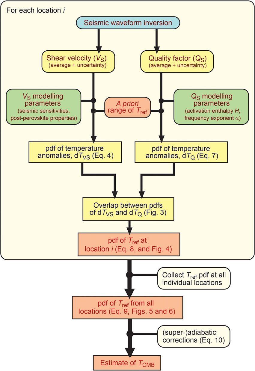
FIGURE 1. Flow chart of the method used to evaluate the temperature at the CMB, T_CMB, from observed shear velocity (V_S) and seismic quality factor (Q_S) measurements at different locations i. For each location, we first calculate a probability density function (pdf) of the average temperature in the layer above the CMB, T_ref, by comparing the pdfs of temperature anomalies predicted by the deviations of V_S and Q_S from PREM. We then combine the local pdfs of T_ref to calculate a total pdf of T_ref. Finally, because T_ref is sampling a layer whose thickness is fixed by the resolution of seismic models, we make a correction for adiabatic and super-adiabatic temperature increase throughout this layer.

2.1 Constraint from shear-wave velocity anomalies

At a given depth, shear-wave velocity anomalies with respect to a reference velocity, dlnV_S, may be expressed as a function of changes in temperature, composition, and phase with respect to the average (or reference) values of these parameters. Because phase changes depend on the pressure and temperature, the contributions of a phase change to dlnV_S implicitly depend on both the local and reference temperatures, T and T_ref. In the lowermost mantle bridgmanite, the most abundant minearal of the lower mantle, may transform its high-pressure phase, post-perovskite (pPv; Oganov and Ono, 2004; Tsuchiya et al., 2004). Mineral physics data indicate that in regions where pPv is present shear waves travel faster than in regular (bridgmanite dominated) mantle. Available measurements are relatively dispersed (see Cobden et al., 2015 for a compilation), but show that, on average, shear velocity increases by 2–3% as bridgmanite transforms to pPv. Due to its large Clapeyron slope, in the range 8–13 MPa/K (Cobden et al., 2015), the depth at which this phase transition occurs strongly depends on temperature and may thus sharply vary in space. In addition, pPv may transform back to bridgmanite a few kilometers or tens of kilometers above the CMB (Hernlund et al., 2005). As a result, the thickness of the pPv lens may strongly vary from one place to another. Radial and lateral parameterizations of seismic models imply that pPv might not be present everywhere in the region sampled by the seismic data. It is therefore meaningful to define a local fraction of pPv, X_pPv. Changes in the local fraction of pPv, for instance due to variations in the thickness of pPv lens, may then contribute to lateral changes in seismic velocities. One may further define a local anomaly in pPv fraction anomaly, dX_pPv, from the difference between the local and reference (i.e., horizontally averaged) fractions of pPv, which depend on T and T_ref.

Assuming that only temperature changes and related changes in the stability field of pPv are present, the temperature anomaly deduced from observed dlnV_S is

${dT}_{V_S}=\frac{\left(\mathrm{d}\mathrm{l}\mathrm{n}{V}_S-S_{pPv}{dX}_{pPv}\right)}{S_T},(1)$

where S_T and S_pPv are sensitivities of shear-wave velocity to temperature and pPv, respectively, defined as the logarithmic partial derivatives of shear-velocity with respect to temperature and pPv. Sensitivities may be deduced from mineral physics data and equation of state modelling. Taking into account dispersion and error bars in mineral physics data provides both means and uncertainties in these sensitivities. For calculations (Section 3), mean and uncertainties in S_T are taken from Deschamps et al. (2012) and mean and uncertainties in S_pPv are deduced from the compilation of Cobden et al. (2015) (Table 2). With these values, a 500 K temperature increase induces a reduction in shear velocity anomaly between 1.2 and 1.5%, and the transition from bridgmanite to pPv triggers a shear velocity increase between 0.1 and 4.6%. Again, the resolution of seismic models implies that pPv may not be present throughout the region sampled by seismic data, implying that the contribution of the pPv phase change to the observed seismic velocity anomalies is a fraction of the velocity change measured by mineral physics data.

Transformation of bridgmanite to pPv occurs over a narrow range of temperature, or thermal width, centered on temperature T_pPv. Here, we describe the local fraction of pPv (between 0 and 1) at temperature T with

$X_{pPv}=\frac{1}{2}\left[1-\tanh \left(\frac{T-T_{pPv}}{\delta T_{pPv}}\right)\right],(2)$

where T_pPv is, again, the temperature of the transition to pPv, and δT_pPv is a typical temperature anomaly modeling the thermal width of the phase transition. Compilation of experimental and ab initio data (Cobden et al., 2015) suggests that at the bottom of the mantle T_pPv may range from 3,000 to 4500 K. Following Eq. 2, and taking T_pPv = 3500 K and δT_pPv = 20 K, X_pPv goes to one for temperatures lower than 3450 K, and to zero for temperatures larger than 3550 K.

Because the distribution of pPv depends on the distribution of temperature, we defined the pPv reference (or horizontally averaged) fraction, X_pPv,ref, according to the lowermost mantle distribution in temperature anomaly, dT = T - T_ref, obtained by Mosca et al. (2012). Noting that this distribution is nearly bimodal (as two peaks can clearly be distinguished; Figure 2A), we first modeled these anomalies with the normalized sum f of two Gaussian distributions. For a given T_ref, we then modulate the fraction of pPv associated with a temperature anomaly dT with the function f (dT), and sum these modulated values over a range of temperature ΔT following

$X_{pPv,ref}\left(T_{ref}\right)={\displaystyle \sum }_{-∆T/2}^{∆T/2}\frac{1}{2}\left[1-\tanh \left(\frac{T_{ref}+dT-T_{pPv}}{\delta T_{pPv}}\right)\right]f\left(dT\right).(3)$

FIGURE 2

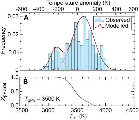
FIGURE 2. (A) Observed (histograms) and modelled (thick red curve) distributions of temperature anomalies from Mosca et al. (2012). The modelled distribution is given by the normalized sum of two Gaussian distributions (thin orange curves), based on the fact that the observed distribution is nearly bimodal. The amplitude, mean and standard deviations of these Gaussian are A₁ = 2.987×10^–2, dT₁ = 60 K, σ₁ = 110 K, and A₂ = 1.173×10^–2, dT₂ = -225 K, σ₂ = 60 (K) (B) Reference fraction of post-perovskite, X_pPv,ref, calculated by Eq. 3 with T_pPv = 3500 K and δT_pPv = 20 (K)

Figure 2B shows X_pPv,ref as a function of T_ref for ΔT = 3000 K and T_pPv = 3500 K. For lower (higher) values of T_pPv, X_pPv,ref is similar to the curve plotted in Figure 2B, but shifted towards lower (higher) T_ref.

Noting that dX_pPv = X_pPv–X_pPv,ref and replacing X_pPv by its expression in Eq. 2, Eq. 1 provides an expression for dT_VS as a function of dlnV_S and T_ref,

$d{T}_{V_S}=\frac{\text{dln}{V}_S}{S_T}-\frac{S_{pPv}}{2S_T}\left[1-\tanh \left(\frac{T_{ref}+d{T}_{VS}-T_{pPv}}{\delta T_{pPv}}\right)-2X_{pPv,ref}\right],(4)$

where X_pPv,ref is given by Eq. 3. Note that the temperature anomaly in Eq. 3 is a summation (dummy) variable specific to this equation, and is therefore different from the dT_VS that we aim to determine. Equation 4 can then easily be solved for dT_VS using classical zero-search methods.

2.2 Constraint from seismic attenuation

The presence of small defects in the crystalline structure of mantle rocks results in the dissipation of a small fraction of the energy carried by seismic waves, leading, in turn, to seismic attenuation as these waves travel through the mantle. Attenuation depends on the frequency of seismic waves and is high only within a range of frequencies, or absorption band (Anderson and Given, 1982). In addition, it is a thermally activated process with a relaxation time that is well described by an Arrhenius law (Anderson and Given, 1982). Practically, seismic attenuation is measured with the quality factor Q. The higher the attenuation, the lower Q. Assuming that it follows a power-law with exponent α of the frequency ω and of the relaxation time (Minster and Anderson, 1981), the quality factor may be written

$Q=Q_0{\omega }^{\alpha }\exp \left(\alpha \frac{H}{RT}\right),(5)$

where Q₀ is a constant, R = 8.32 Jmol⁻¹K⁻¹ the ideal gas constant, T the temperature, and H = E + pV the activation enthalpy, with E and V being the activation energy and volume, respectively, and p the pressure.

We model the anomaly in quality factor with respect to a reference value Q_ref following the approach of Deschamps et al. (2019). Eq. 5 may be used model the quality factor at any temperature T, including at a reference temperature T_ref, which defines the reference quality factor Q_ref. Noting dT_Q the temperature anomaly (T - T_ref) at a location where Q_S is measured, we define the anomaly in shear quality factor with the ratio between Q_S and Q_ref,

$\frac{Q_S}{Q_{ref}}=\exp \left[\alpha \frac{H}{R{T}_{ref}}\left(\frac{T_{ref}}{T_{ref}+d{T}_Q}-1\right)\right].(6)$

Inversion of Eq. 6 gives dT_Q from Q_S following,

$d{T}_Q=-\frac{R{T_{ref}}^2}{\alpha H}\frac{\ln \left(\frac{Q_S}{Q_{ref}}\right)}{\left[1+\frac{R{T}_{ref}}{\alpha H}\ln \left(\frac{Q_S}{Q_{ref}}\right)\right]}.(7)$

For calculations, we set Q_ref to its PREM value in the lower mantle, which is equal to 312 (Dziewonski and Anderson, 1981) and is consistent with models built from a probabilistic approach (Resovsky et al., 2005). A difficulty is that the values of α and H are poorly constrained. At lowermost mantle depths α was found to be equal to 0.1 for periods in the range 300–800 s, and around 0.3 for a period of 200 s (Lekić et al., 2009). In their anelastic model Dannberg et al. (2017) used α = 0.274 to fit the shear-wave velocity of PREM (Dziewonski and Anderson, 1981) and the quality factor of QL6 (Durek and Ekström, 1996). Dannberg et al. (2017) further used activation energy and volume activation equal to 286 kJ/mol and (1.2 ± 0.1)×10^–6 m³/mol, respectively, leading to activation enthalpy at the bottom of the mantle around 440 kJ/mol. Possible range of these two parameters are however larger and may lead to values of H in the range 250–900 kJ/mol (for discussion on E and V values, see Matas and Bukowinski, 2007 and supplementary material of Deschamps et al., 2019). Interestingly, Eq. 7 indicates that only the product αH matters for calculations of dT_Q. Here, we explored values of this product in the range 20–400 kJ/mol, covering conservative ranges of α and H, 0.1–0.4 and 200–1,000 kJ/mol, respectively.

Attenuation may be affected by the presence of volatiles, most particularly water. The amount of water in the deep mantle may however be very limited, less than about 30 ppm weight in bridgmanite (Panero et al., 2015). For such low concentrations, rocks may be considered as dry, and volatiles would have no or very limited effects. This hypothesis is further supported by recent mineral physics experiments on olivine showing that for water contents relevant to the Earth’s interior, attenuation and seismic velocities are not sensitive to the water content (Cline et al., 2018). Finally, attenuation of mantle minerals may also be sensitive to grain size. Jackson et al. (2002) quantified this effect for olivine, but to date the grain size sensitivities of lower mantle minerals remain unconstrained. Using olivine data and an extended Burgers model (Faul and Jackson, 2015), Lau and Faul (2019) showed that grain-size may affect attenuation at lower mantle pressures and periods ranging from seismic to tidal timescales. For periods around 10 s, their results further indicate that grain-size dependence is reduced as pressure increases (see their Figure 5), suggesting no or limited grain-size dependence close to the CMB. In addition, because grain-size dependence is controlled by a grain-size exponent, and since we quantify anomalies in quality factor as the ratio between local and reference quality factors (Eq. 6), grain-size effects should not affect dT_Q provided that the grain-size does not vary substantially at a given depth.

2.3 Probability density functions of the reference temperature T_ref

The request that, at a given location, the dT_VS and dT_Q deduced from Eqs. 4 and Eq. 7 are equal provides, in principle, an estimate of T_ref. However, depending on the observed dlnV_S and Q_S and on the assumed values of the model parameters (mainly α, H, and T_pPv), dT_VS = dT_Q may have more than one solution or no solution at all. To solve this issue, we follow an approach based on distributions of dT_VS and dT_Q as a function of T_ref, which further allow to take into account uncertainties on observed data. For a set of dlnV_S and Q_S measured at different locations, we then obtain a probability density function (pdf) for an a priori range of T_ref. The different steps leading to such pdfs are detailed below.

We first estimate distributions in dT_VS and dT_Q at a given location i and reference temperature T_ref. For this, we randomly vary observed dlnV_S and Q_S around their average values following Gaussian distributions with prescribed standard deviations. For each sample we then calculate the corresponding dT_VS and dT_Q, and bin these temperature anomalies in normalized frequency histograms, leading to individual pdfs, $P_{\text{VS}}^i$ and $P_{\mathrm{Q}}^i$. Figure 3 plots example of such pdfs built from a set of 1 million dlnV_S and Q_S samples for Central America location S2 (Table 1) and for different values of T_ref. Standard deviations for dlnV_S and Q_S are fixed to the estimated uncertainties in these data, which are here equal to 0.1% and 20, respectively, and the values of parameters in Eqs. 4 and Eq. 7 are listed in Table 2. Interestingly, dT_Q pdfs are Gaussian with a good approximation. If the pPv anomaly (dX_pPv) is null, dlnV_S is only due to temperature changes, and dT_VS pdfs are also nearly Gaussian. By contrast, distributions in dT_VS strongly deviate from Gaussian distributions if the local pPv fraction is different from its horizontally average (dX_pPv is different from zero).

FIGURE 3

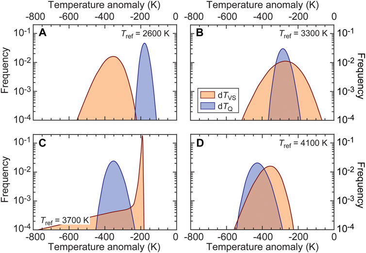
FIGURE 3. Probability density functions of temperature anomalies deduced from dlnV_S (dT_VS, orange distributions) and Q_S (dT_Q, blue distributions) measured in corridor S2 beneath Central America (see Borgeaud and Deschamps 2021 for the exact location). Mean and standard deviation in dlnV_S and Q_S are 1.0% and 0.1% and 470 and 20, respectively (Table 1), and different reference temperature T_ref are considered in each plot: 2600 K (A); 300 K (B); 3700 K (C); and 4100 K (D). Other modeling parameters are set to their preferred values listed in Table 2. The overlap between the pdfs for dT_VS and dT_Q at a specific value of T_ref is taken as a measure of the probability p that T_ref is equal to this specific value. The transition temperature to post-perovskite is set to T_pPv = 3500 K. Note that the frequency (y-axis) is plotted in logarithmic scale.

TABLE 1

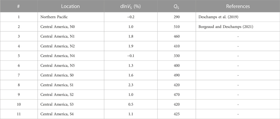
TABLE 1. Values of shear velocity anomalies (dlnV_S) and attenuation (Q_S) used to estimate the CMB temperature, T_CMB. Values of dlnV_S are with respect to the PREM (Dziewonski and Anderson, 1981) value in the lowermost 50 km, V_PREM = 7.26 km/s.

TABLE 2

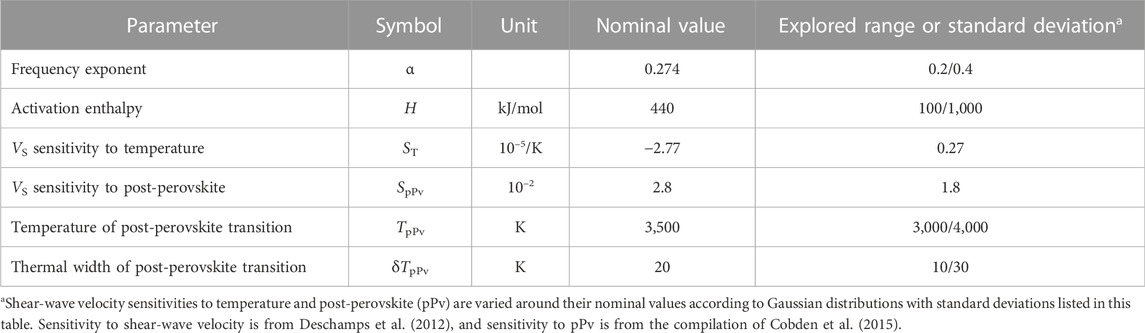
TABLE 2. Modeling parameters for the calculation of temperature anomalies deduced from dlnV_S (Eq. 4) and Q_S (Eq. 7). See text and methods for the definition of these parameters.

We then define the likelihood that T_ref is equal to a specific value by the overlap between the integrals of the distributions obtained for dT_VS and dT_Q (see Figure 3), which, for location i, may be expressed as

$P_{Tref}^i=C_n^i\underset{d{T}_0}{\overset{d{T}_1}{{\displaystyle \int }}}\min \left(P_{\text{VS}}^i\left(T_{\text{ref}}\right),P_{\mathrm{Q}}^i\left(T_{\text{ref}}\right)\right)d\left(dT\right),(8)$

where dT₀ and dT₁ are the assumed lower and upper bounds in temperature anomaly, $\Delta T=\left(d{T}_1-d{T}_0\right)$, and $C_n^i$ a normalisation constant obtained by summing $P_{Tref}^i$ over the entire explored ranges of T_ref and, if applying, other parameters (for instance the product αH). Eq. 8 can be used to estimate likelihoods at all locations where joint measurements of dlnV_S and Q_S are available. The products of these local likelihoods for each value of T_ref finally provide an estimate of the likelihood for each value of T_ref,

$P_{Tref}={\displaystyle \prod }_{i=1}^N{P}_{Tref}^i,(9)$

where N is the number of locations for which measurements are available.

2.4 Corrections for radial averaging

Strictly speaking our method provides an estimate of the average temperature within the mantle lowermost few tens of kilometers, the exact thickness of this layer depending on the radial resolution of the observed V_S and Q_S. It can however give access to T_CMB provided that a small correction ΔT_z is applied to account for the temperature increase within this layer. This increase includes an adiabatic contribution due to the pressure increase, and a super-adiabatic temperature increase due to the presence at the bottom of the mantle of a thermal boundary layer associated with mantle convection. Practically, and ignoring the effects of spherical geometry, the horizontally averaged temperature obtained by the method described in the previous sections may be written $T_{ref}=\frac{1}{2}\left(T_{top}+T_{CMB}\right)$, where T_top is the temperature at the top of the sampled layer. Noting that $T_{CMB}=T_{top}+∆T_z$, one gets $T_{CMB}=T_{ref}+∆T_z/2$. As an illustration, for models of V_S and Q_S with a radial resolution of 50 km, and assuming adiabatic and super-adiabatic temperature gradient of 0.3 K/km and 2.5 K/km (typical of the gradient obtained in numerical simulations of mantle convection), respectively, ΔT_z is about 140 K and a correction of 70 K should be applied.

3 A preliminary estimate

We applied the method detailed in section 2 to the measurements of V_S and Q_S listed in Table 1. Our goal is not to provide a conclusive value for the CMB temperature, as more measurements of V_S and Q_S together with a transition temperature to pPv more precise than current estimates may be needed for this, but rather to test our method. The measurements of V_S and Q_S we used are the lowermost layer of 1D radial profiles obtained beneath the Northern Pacific (Deschamps et al., 2019) and beneath Central America (Borgeaud and Deschamps, 2021) by full-waveform inversions of seismic data. In both cases, the inversion method is similar to that used in Konishi et al. (2017), and the radial resolution of the 1D models is 50 km, i.e. the V_S-anomalies and Q_S in Table 1 sample a 50 km thick layer above the CMB. Note that the method used to recover Central America profiles further includes travel-time corrections for the 3D mantle structure beneath Central America, spectral amplitude misfit to better constrain Q_S, and corrections for focusing effects in the lowermost mantle (Borgeaud and Deschamps, 2021). We converted V_S to relative anomalies dlnV_S with respect to PREM (Dziewonski and Anderson, 1981) shear-wave velocity, which, in the lowermost 50 km, is equal to 7.26 km/s. We then built dT_VS and dT_Q distributions for values of T_ref in the range 2,500–4500 K by randomly generating 1 million dlnV_S and Q_S samples at each T_ref. Samples distributions follow Gaussian distributions centered on the observed dlnV_S and Q_S and with standard deviations fixed to 0.1% for dlnV_S and 20 for Q_S, on the basis of observed error bars. Values of the modelling parameters used in Eqs 4, 7 are listed in Table 2. In particular, we explored values of the frequency exponent, α, and activation enthalpy, H, of attenuation in ranges leading to values of the product αH between 20 and 400 kJ/mol. Because temperature of the transition to pPv, T_pPv, is uncertain, and to quantify its influence on T_ref, we performed calculations for several values of this parameter in the range 3,000–4250 K.

Left column in Figure 4 shows the median in dT_VS and dT_Q (defined as the 0.5 pdf quartile, meaning that there is 50% likelihood that T_ref lie on each side of this value) as a function of T_ref and at different locations. Modeling parameters are fixed to T_pPv = 3500 K, α = 0.274, and H = 440 kJ/mol. The coloured areas cover 68.3% of the pdfs around their median values, which, for Gaussian distributions, correspond to one standard deviation. Right column plots the corresponding likelihood normalized with the maximum likelihood, P_max, for each case. The evolution of dT_VS as a function of T_ref is controlled by the anomaly in the fraction of pPv, dX_pPv. If T_ref is too low or too large, pPv is either fully covering the CMB (X_pPv,ref = 1) or nowhere stable (X_pPv,ref = 0). In both cases dX_pPv = 0 and dlnV_S is only affected by the temperature anomaly, implying that dT_VS does not depend on T_ref. The lower (T_low) and upper (T_up) bounds of temperature for a non-zero dX_pPv are depending on both the assumed lower mantle temperature distribution and T_pPv. Taking the temperature distribution from Mosca et al. (2012) and T_pPv = 3500 K, these bounds are around T_low = 3000 K and T_up = 4000 K (Figure 2B). For intermediate temperatures, an excess (deficit) in pPv triggers an increase (decrease) in seismic velocity, such that part of the observed dlnV_S is due to the pPv anomaly. As a result, for locations colder than the reference temperature, dT_VS is lower (in absolute value) than its purely thermal value if dX_pPv > 0, and larger if dX_pPv < 0. For location hotter than T_ref, the opposite trends occur. Note that discontinuity in dT_VS may occur (for instance, corridor N1 in Central America) as the dX_pPv falls to zero for T_ref ≤ T_low or T_ref ≥ T_up. For each location, overlaps between dT_VS and dT_Q distributions at a given value of T_ref provide an estimate of the likelihood for this specific value of T_ref, with larger overlaps leading to higher likelihoods (Section 2.3). For locations with V_S and Q_S close to PREM (for instance, Northern Pacific and corridor N4 in Central America), overlap between dT_VS and dT_Q occur for a wide range of T_ref. Implying that these locations bring few constraints to T_ref. The distributions in dT_VS further depend on the assumed value of T_pPv, which, again, is fixed to 3500 K in Figure 4. For higher (lower) T_pPv, these distributions keep the same shape but shifts to larger (smaller) T_ref. In other words, and as one would expect, higher T_pPv favors higher T_ref. Similarly, the distributions in dT_Q depends on the product αH, with temperature anomalies getting smaller (blue curves in Figure 4 move towards dT_Q = 0) as αH increases. The sign of dT_Q, on another hand, is controlled by the ratio between the observed and reference quality factors, Q_S/Q_ref.

FIGURE 4

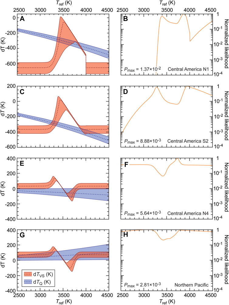
FIGURE 4. Distribution in dT_VS and dT_Q (left column) and corresponding likelihoods (right column) as a function of T_ref and at different locations: Central America N1 (A,B); Central America S2 (C,D); Central America N4 (E,F); and Northern Pacific (G,H). Dashed curves in distribution plots show the median (defined as the 0.5 pdf quartile, i.e., T_ref lie on each side of this value with a 50% likelihood) in dT_VS and dT_Q, and the coloured areas cover 68.3% of the pdfs around their median values. Likelihood (right column) are normalized with their maximum values and plotted with a logarithmic scale. The frequency exponent, activation enthalpy, and transition temperature to pPv are set to α = 0.274, H = 440 kJmol^-1, and T_pPv = 3500 K. For other details of the calculations, see text and Table 2.

Figure 5A plots the total likelihood (Eq. 9), defined as the product of individual local likelihoods, obtained for T_pPv =3500 K as a function of both T_ref and the product αH. For clarity, we also show in Figure 6 likelihoods for selected values of αH. Interestingly, the most likely range of T_ref depends relatively little on αH. For αH ≤ 100 kJ/mol, likelihood is very low (at least one order of magnitude lower than the maximum likelihood) whatever the value of T_ref, suggesting that such values of αH can be ruled out. Above this value, the most likely T_ref slightly decreases with increasing αH, from ∼3800 K at αH = 100 kJ/mol, to ∼3600 K at αH = 400 kJ/mol. Likelihood is largest for αH around 140 kJ/mol, but remains high throughout the range 100–400 kJ/mol (Figure 6; note the logarithmic scale). High likelihood may still be found for αH ≥ 400 kJ/mol (not explored in this study), but this would imply values of α and H in excess of 0.4 and 1,000 kJ/mol, respectively, which appear unlikely (Section 2.2). We did another calculation using the temperature distribution of Trampert et al. (2004) to calculate X_pPv,ref (and therefore dX_pPv; Section 2.1), but did not find substantial differences in the total likelihood (Figure 5B). By contrast, and as one would expect, T_pPv has a strong impact on the estimated likelihood, the most likely value of T_ref increasing with T_pPv (see plots c and d in Figure 5, obtained for T_pPv equal to 3,000 and 4000 K, respectively). Note also that lower values of T_pPv allow lower values of αH. Following our approach, a precise inference of T_ref therefore requires an accurate knowledge of T_pPv.

FIGURE 5

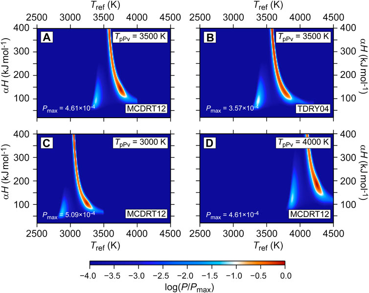
FIGURE 5. Total likelihood (P, color scale), given by Eq. 9, as a function of the reference temperature (x-axis) and of the product of the frequency exponent α and activation enthalpy H (y-axis). Three values of the transition temperature to post-perovskite (pPv), T_pPv, are considered, 3500 K (A,B), 3000 K (C), and 4000 K (D). The temperature distribution used to model the pPv average fraction is either from Mosca et al. (2012) [plots (A,C,D)] or Trampert et al. (2004) (B). Other modeling parameters are listed in Table 2. In all cases, likelihoods are normalized with their maximum value P_max over the range of explored T_ref and αH, and plotted with logarithmic scale.

FIGURE 6

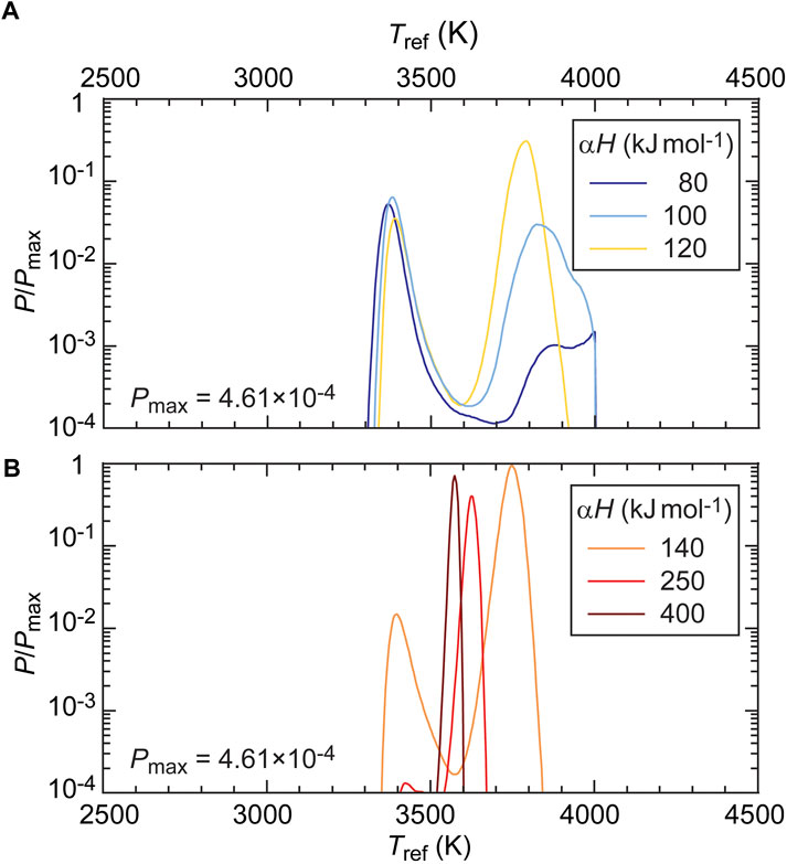
FIGURE 6. Total likelihood, defined as the product of the individual likelihood at each location (Eq. 9), as a function of the reference temperature T_ref and for several values of the product of the frequency exponent α and activation enthalpy H: 80, 100, and 120 kJ mol⁻¹ (A); and 140, 250, and 400 kJ mol⁻¹ (B). Total likelihoods are normalized with the absolute maximum, P_max, and plotted with a logarithmic scale. The temperature of the transition to pPv is T_pPv = 3500 K. For other details of the calculations, see text and Table 2.

To estimate the most likely range of T_ref we summed up obtained likelihoods over the explored range of αH, and calculated cumulative likelihoods (Figure 7; note the logarithmic scale in plot a). For T_pPv = 3500 K, the summed likelihood has two peaks, around T_ref = 3600 K and T_ref = 3750 K. The cumulative likelihood indicates that T_ref lies within the range 3,400–3810 K with a 95% likelihood, and that its median value, defined as the 0.5 quartile (meaning that there is 50% likelihood that T_ref lies on each side of this value), is around 3650 K. Again, for larger (lower) values of T_pPv, these range and median value both shift to higher (lower) values. Figure 8, plotting the median value of T_ref as a function of T_pPv, shows that the median T_ref increases nearly linearly with T_pPv. The grey band in Figure 8 covers values of T_ref ranging from quartiles 0.025 to 0.975, meaning, again, that there is 95% likelihood that T_ref lies within this range. As discussed in section 2.4, T_ref is an estimate of the reference temperature averaged out in the mantle lowermost 50 km. Adding the estimated adiabatic and super-adiabatic temperature jumps to the median T_ref, the CMB temperature may be given by

$T_{CMB}=a_0+a{T}_{pPv}+∆T_z/2.(10)$

FIGURE 7

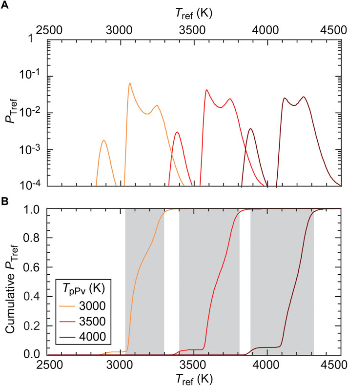
FIGURE 7. (A) Likelihood summed over the explored range of αH as a function of T_ref and for three values of T_pPv (color code). (B) Cumulative likelihood for the three cases shown in plot (A). The gray shaded bands cover quartiles 0.025 to 0.975, and therefore indicate the range of temperature within which T_ref has a 95% likelihood to lie.

FIGURE 8

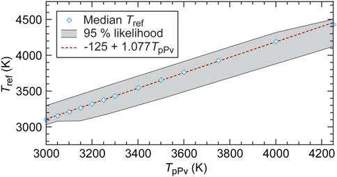
FIGURE 8. Reference temperature in the lowermost 50 km of the mantle, T_ref, estimated from attenuation and shear velocity measured beneath Central America (Borgeaud and Deschamps, 2021) and the Northern Pacific (Deschamps et al., 2019) as a function of the transition temperature to post-perovskite, T_pPv. The crosses show T_ref median values, meaning that there is 50% likelihood that T_ref is on each side of this value. The dashed red curve shows the linear fit to these median values, and the gray area covers values of T_ref ranging from quartiles 0.025 to 0.975, i.e., the likelihood that T_ref is within this range is 95%. The CMB temperature may be estimated by adding a small depth correction to T_ref (Section 2.4 and Eq. 10).

A least square fit of our calculations for T_pPv in the range 3,000–4250 K leads to a₀ = -125 K and a = 1.077. For instance, taking T_pPv = 3500 K and ΔT_z = 140 K (Section 2.4) leads to a CMB temperature of 3715 K and a 95% likelihood range of 3,470–3880 K.

4 Discussion and concluding remarks

In this study, we built a method to infer CMB temperature (T_CMB) from measurements of seismic shear-wave velocity (V_S) and quality factor (Q_S) in the lowermost mantle. Both these two observables bring constraints on the local temperature anomaly with respect to a horizontally averaged temperature T_ref, and the combination of these constraints provides estimates of T_ref at that depth. A correction for radial averaging related to the radial resolution of V_S and Q_S then gives T_CMB. To account for uncertainties in the modelling parameters of V_S and Q_S, our method calculates probability density functions (pdfs) of T_ref (and thus T_CMB), rather than mean, single values. Because it is based on the fact that seismic velocity is affected by lateral changes in the depth of the phase transition from bridgmanite to post-perovskite (pPv), and therefore by lateral changes in the amount of pPv at a given location, the pdfs of T_ref deduced from our approach depend on the transition temperature from bridgmanite to pPv close to the CMB, T_pPv. Applying our method to measurements of V_S and Q_S beneath Central America (Borgeaud and Deschamps, 2021) and the Northern Pacific (Deschamps et al., 2019), we found that for T_pPv = 3500 K the CMB temperature should be in the range 3,470–3880 K with a 95% likelihood.

Because in our approach the value of T_CMB depends on the value of T_pPv right above the CMB, which remains poorly known, comparison between our results and available estimates is not straightforward. It is however interesting to note that the range of T_CMB we obtained for T_pPv = 3500 K (grey shaded area in Figure 9), is coherent with the upper range of T_CMB estimated from radial seismic velocity profiles to which a 500 K amplitude thermal boundary layer (TBL) is added, with the maximum possible T_CMB deduced from the solidus of pyrolite, and with the lower bound of the range of T_CMB estimated from the melting temperature T_ICB of iron alloys at the inner core boundary. Figure 9, further indicate possible ranges of T_pPv (according to Eq. 10) for T_CMB obtained by different methods. For instance, the range of T_CMB estimated from the pyrolite solidus and from T_ICB implies T_pPv from 3,350 to 3950 K, and 3,600–4300 K, respectively. The values of T_pPv compatible with the CMB temperatures inferred from seismic profiles are overall lower, but depend on the assumed thermal amplitude of the TBL added to the adiabatic temperatures deduced from these profiles. For ΔT_TBL = 500 K, T_pPv is in the range 2,800–3500 K, i.e., and as one would expect, on the lower range of experimental measurements.

FIGURE 9

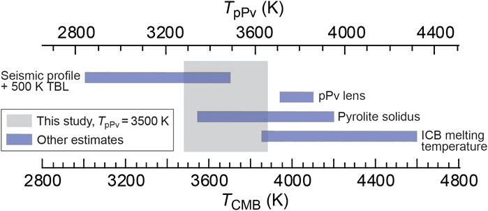
FIGURE 9. Comparison between our results and CMB temperatures, T_CMB (bottom scale), estimated from radial seismic profiles, post-perovskite (pPv) lenses, pyrolite solidus at the CMB, and measurements of iron alloys melting temperature at the inner core boundary. The top scale shows the pPv transition temperature at the CMB, T_pPv, calculated by inverting Eq. 10. The gray area covers the range of T_CMB (95% likelihood) we obtained for T_pPv = 3500 K (the range of uncertainty does not apply to the top scale).

Certainly the biggest unknown in our modelling is T_pPv, which at the CMB may range from 3,000 to 4500 K (Cobden et al., 2015). A complication is that the exact transition temperature depends on the composition of the aggregate. For instance, higher iron content within bridgmanite increases T_pPv, while aluminium has the opposite effect. In addition, laboratory experiments are made at fixed pressures, and extrapolation to the CMB requires knowledge of the Clapeyron slope, Γ_pPv, which may range between 8 and 13 MPa/K. For pyrolytic compositions and a temperature of 2500 K, transition to pPv is usually observed in the pressure range 115–130 GPa (Ohta et al., 2008; Catalli et al., 2009; Sinmyo et al., 2011), which, assuming Γ_pPv = 10 MPa/K leads to T_pPv in the range 3,000–4500 K close to the CMB. Still for pyrolytic composition, the recent experiments of Kuwayama et al. (2021) favor a low Clapeyron, 6.5 ± 2.2 MPa/K, and a T_pPv in excess of 4000 K. If our approach is correct, too large value of T_pPv may however be difficult to reconcile with experimental solidus of pyrolite (Fiquet et al., 2010; Andrault et al., 2011; Nomura et al., 2014), as it would lead to CMB temperatures in excess of this solidus. Alternatively, T_CMB may be lower than predicted by our approach (Figure 8), in which case pPv may be present all around the CMB. This, however, is difficult to reconcile with the values of V_S and Q_S observed beneath Central America, which cannot be explained by temperature changes only and instead require changes in the depth of the pPv lens lower boundary (Borgeaud and Deschamps, 2021). Other modelling parameters, most particularly the frequency exponent and activation enthalpy of the quality factor, α and H, are still poorly known (Section 2.2). Because it depends on the product αH, and not on individual values of α and H, our approach can accommodate part of these uncertainties. In addition, the recovered T_ref depends only slightly on this product (Figure 5). Nevertheless, more precise values of α and H would refine the possible range of T_ref for a given T_pPv.

Our approach implicitly assumes that seismic velocity is not affected by the presence of compositional changes. Unless the compositional effects and their contributions to V_S-anomalies are well identified and quantified, thus allowing to correct V_S, our method may not be applied to measurements obtained within regions that are chemically different from the average (pyrolytic) mantle. This is likely the case of large low shear-wave velocity provinces (LLSVPs) observed in the lowermost mantle beneath Africa and the Pacific (e.g., Garnero et al., 2016), and which are thought to be regions simultaneously hotter than average mantle and chemically differentiated, possibly enriched in iron by a few percent (e.g., Trampert et al., 2004; Deschamps et al., 2012; Mosca et al., 2012). Mineral physics data indicate that shear velocity decreases with increasing iron content. Following the seismic sensitivities to iron from Deschamps et al. (2012), a 3% enrichment in iron decrease shear velocity by 0.8–1.1%. If not accounted for, an excess in iron oxide would then result in overestimated temperature anomalies. Correction for this effect would shift local temperatures, and thus, temperature anomalies, to higher values (red curves in Figure 4 would shift upwards), changing in turn the estimated T_ref. Such corrections however require a precise knowledge of the iron excess, which, to date, is not available. Estimates from seismic normal modes (Trampert et al., 2004; Mosca et al., 2012) suggest an enrichment around 2 to 4 wt%, but these estimates poor of lateral and vertical resolutions. Another potential source of chemical heterogeneities is mid-ocean ridge basalt (MORB) that may be entrained with slabs down to the CMB. This might be the case of the region explored by Borgeaud and Deschamps (2021), which was associated with the subduction of the Farallon slab to the CMB (e.g., Hung et al., 2005; Borgeaud et al., 2017). However, MORBs represent only a thin layer on top of the slab. In addition, if post-perovskite is present in the lowermost mantle, the sensitivity of V_S to MORB may be very small (Deschamps et al., 2012). Overall, the contribution of recycled MORB pieces may be limited and much smaller than that of temperature and post-perovskite changes. Finally, reactions between core molten iron alloys and mantle silicate rocks, if they happen, may also impact seismic velocity anomalies. High pressure experiments indicate that such reactions could be a source of iron alloys (FeO and FeSi; Knittle and Jeanloz, 1991) and iron-aluminum alloy (Dubrovinsky et al., 2001). Core-mantle chemical reactions may then result in local excess in iron oxides, with consequences on the interpretation of shear velocity anomalies similar to those for iron-enriched LLSVPs. To date, however, there is no seismic evidences for the presence of such regions, and no quantitative constraints on the possible excess of iron at these locations.

Finally, the relationship between T_ref and T_pPv we obtained (Figure 8) was built from observations made beneath Central America (Borgeaud and Deschamps, 2021) plus one observation made beneath the Nothern Pacific (Deschamps et al., 2019). Additional measurements obtained in different regions would be needed to confirm this trend, and to avoid potential bias related to the area explored by Borgeaud and Deschamps (2021). Ideally, this would include regions with V_S and Q_S away from PREM values, which do not bring strong constraints, and LLSVPs, for which part of the seismic velocity anomalies may originate from compositional differentiation.

Despite the difficulties discussed in this section and the fact that it relies on an accurate knowledge of T_pPv, the approach we developed in this study offers an alternative way to estimate the CMB temperature. In addition, it may be easily adapted or modified for other purposes, for instance mapping post-perovskite or chemical fields in the deep mantle.

Data availability statement

The original contributions presented in the study are included in the article/Supplementary Material, further inquiries can be directed to the corresponding author.

Author contributions

Project design, code development, and calculations were performed by FD. LC provided expertise on post-perovskite properties. Both authors discussed the method and the results, and participated to the manuscript writing.

Funding

The research presented in this article was supported by Academia Sinica AS-IA-108-M03 and the Ministry of Science and Technology of Taiwan (MoST) grant 110-2116-M-001-025.

Conflict of interest

The authors declare that the research was conducted in the absence of any commercial or financial relationships that could be construed as a potential conflict of interest.

Publisher’s note

All claims expressed in this article are solely those of the authors and do not necessarily represent those of their affiliated organizations, or those of the publisher, the editors and the reviewers. Any product that may be evaluated in this article, or claim that may be made by its manufacturer, is not guaranteed or endorsed by the publisher.

References

Anderson, D. L., and Given, D. W. (1982). Absorption band Q model for the Earth. J. Geophys. Res. 87, 3893–3904. doi:10.1029/jb087ib05p03893

CrossRef Full Text | Google Scholar

Anderson, O. L. (1982). The Earth’s core and the phase diagram of iron. Philos. Trans. R. Soc. Lond. A 306, 21–35.

Google Scholar

Andrault, D., Bolfan-Casanova, N., LoNigro, G., Bouhifd, M. A., Garbarino, G., and Mezouar, M. (2011). Solidus and liquidus profiles of chondritic mantle: Implication for melting of the Earth across its history. Earth Planet. Sci. Lett. 304, 251–259. doi:10.1016/j.epsl.2011.02.006

CrossRef Full Text | Google Scholar

Anzellini, S., Dewaele, A., Mezouar, M., Loubeyre, P., and Morard, G. (2013). Melting of iron at Earth’s inner core boundary based on fast X-ray diffraction. Science 340, 464–466. doi:10.1126/science.1233514

PubMed Abstract | CrossRef Full Text | Google Scholar

Boehler, R. (1993). Temperatures in the Earth’s core from melting-point measurements of iron at high static pressures. Nature 363, 534–536. doi:10.1038/363534a0

CrossRef Full Text | Google Scholar

Borgeaud, A. F. E., and Deschamps, F. (2021). Seismic attenuation and S-velocity structures in beneath central America using 1-D full-waveform inversion. JGR. Solid Earth 126, e2020JB021356. doi:10.1029/2020JB021356

CrossRef Full Text | Google Scholar

Borgeaud, A. F. E., Kawai, K., Konishi, K., and Geller, R. J. (2017). Imaging paleoslabs in the D″ layer beneath Central America and the Caribbean using seismic waveform inversion. Sci. Adv. 3, e1602700. doi:10.1126/sciadv.1602700

PubMed Abstract | CrossRef Full Text | Google Scholar

Brown, J. M., and McQueen, R. G. (1986). Phase transitions, Grüneisen parameter, and elasticity for shocked iron between 77 GPa and 400 GPa. J. Geophys. Res. 91, 7485–7494. doi:10.1029/jb091ib07p07485

CrossRef Full Text | Google Scholar

Brown, J. M., and Shankland, T. J. (1981). Thermodynamic parameters in the Earth as determined from seismic profiles. Geophys. J. Int. 66, 579–596. doi:10.1111/j.1365-246x.1981.tb04891.x

CrossRef Full Text | Google Scholar

Buffet, B. A. (2007). A bound on heat flow below a double crossing of the perovskite-postperovskite phase transition. Geophys. Res. Lett. 34, L17302. doi:10.1029/2007GL030930

CrossRef Full Text | Google Scholar

Catalli, K., Shim, S., and Prakapenka, V. (2009). Thickness and Clapeyron slope of the post-perovskite boundary. Nature 462, 782–785. doi:10.1038/nature08598

PubMed Abstract | CrossRef Full Text | Google Scholar

Cline, C. J., Faul, U. H., David, E. C., Berry, A. J., and Jackson, I. (2018). Redox-influenced seismic properties of upper-mantle olivine. Nature 555, 355–358. doi:10.1038/nature25764

PubMed Abstract | CrossRef Full Text | Google Scholar

Cobden, L. J., Thomas, C., and Trampert, J. (2015). “Seismic detection of post-perovskite inside the Earth,” in The Earth's heterogeneous mantle. Editors A. Khan, and F. Deschamps (Singapore: Springer), 391–440. doi:10.1007/978-3-319-15627-9_13

CrossRef Full Text | Google Scholar

Dannberg, J., Eilon, Z., Faul, U., Gassmöller, R., Moulik, P., and Myhill, R. (2017). The importance of grain size to mantle dynamics and seismological observations. Geochem. Geophys. Geosyst. 18, 3034–3061. doi:10.1002/2017GC006944

CrossRef Full Text | Google Scholar

Davies, C., Pozzo, M., Gubbins, D., and Alfè, D. (2015). Constraints from material properties on the dynamics and evolution of Earth’s core. Nat. Geosci. 8, 678–685. doi:10.1038/ngeo2492

CrossRef Full Text | Google Scholar

Deschamps, F., Cobden, L. J., and Tackley, P. J. (2012). The primitive nature of large low shear-wave velocity provinces. Earth Planet. Sci. Lett. 349-350, 198–208. doi:10.1016/j.epsl.2012.07.012

CrossRef Full Text | Google Scholar

Deschamps, F., Konishi, K., Fuji, N., and Cobden, L. J. (2019). Radial thermo-chemical structure beneath Western and Northern Pacific from seismic waveform inversion. Earth Planet. Sci. Lett. 520, 153–163. doi:10.1016/j.epsl.2019.05.040

CrossRef Full Text | Google Scholar

Deschamps, F., and Trampert, J. (2004). Towards a lower mantle reference temperature and composition. Earth Planet. Sci. Lett. 222, 161–175. doi:10.1016/j.epsl.2004.02.024

CrossRef Full Text | Google Scholar

Dubrovinsky, L., Annersten, H., Dubrovinskaia, N., Westman, F., Harryson, H., Fabrichnaya, O., et al. (2001). Chemical interaction of Fe and Al₂O₃ as a source of heterogeneity at the Earth’s core-mantle boundary. Nature 412, 527–529. doi:10.1038/35087559

PubMed Abstract | CrossRef Full Text | Google Scholar

Durek, J. J., and Ekström, G. (1996). A radial model of anelasticity consistent with long-period surface wave-attenuation. Bull. Seismol. Soc. Am. 86, 144–158.

Google Scholar

Dziewonski, A. M., and Anderson, D. L. (1981). Preliminary reference Earth model. Phys. Earth Planet. Interiors 25, 297–356. doi:10.1016/0031-9201(81)90046-7

CrossRef Full Text | Google Scholar

Faul, U. H., and Jackson, I. (2015). Transient creep and strain energy dissipation: An ex-perimental perspective. Annu. Rev. Earth Planet. Sci. 43, 541–569. doi:10.1146/annurev-earth-060313-054732

CrossRef Full Text | Google Scholar

Fiquet, G., Auzende, A. L., Siebert, J., Corgne, A., Bureau, H., Ozawa, H., et al. (2010). Melting of peridotite to 140 gigapascals. Science 329, 1516–1518. doi:10.1126/science.1192448

PubMed Abstract | CrossRef Full Text | Google Scholar

Fischer, R. A., Campbell, A. J., Reaman, D. M., Miller, N. A., Heinz, D. L., Dera, P., et al. (2013). Phase relations in the Fe-FeSi system at high pressures and temperatures. Earth Planet. Sci. Lett. 373, 54–64. doi:10.1016/j.epsl.2013.04.035

CrossRef Full Text | Google Scholar

Fischer, R. A. (2016). “Melting of Fe alloys and the thermal structure of the core,”. Deep Earth Phys. Chem. Low. Mantle CoreEditors H. Teresaki, and R. A. Fischer (Geophysical Monograph), 217, 3–12.

CrossRef Full Text | Google Scholar

Frost, D. A., Avery, M. S., Buffet, B. A., Chidester, B. A., Deng, J., Dorfman, S. M., et al. (2022). Multidisciplinary constraints on the thermo-chemical boundary between Earth’s core and mantle. Geochem. Geophys. Geosys. 23, e2021GC009764. doi:10.1029/2021GC009764

CrossRef Full Text | Google Scholar

Garnero, E. J., McNamara, A., and Shim, S.-H. (2016). Continent-sized anomalous zones with low seismic velocity at the base of Earth’s mantle. Nat. Geosci. 9, 481–489. doi:10.1038/ngeo2733

CrossRef Full Text | Google Scholar

Hernlund, J., Thomas, C., and Tackley, P. J. (2005). A doubling of the post-perovskite phase boundary and structure of the Earth’s lowermost mantle. Nature 434, 882–886. doi:10.1038/nature03472

PubMed Abstract | CrossRef Full Text | Google Scholar

Hung, S.-H., Garnero, E. J., Chiao, L.-Y., Kuo, B.-Y., and Lay, T. (2005). Finite frequency tomography of D″ shear velocity heterogeneity beneath the Caribbean. J. Geophys. Res. 110, B07305. doi:10.1029/2004jb003373

CrossRef Full Text | Google Scholar

Jackson, I. (1998). Elasticity, composition and temperature of the Earth’s lower mantle: A reappraisal. Geophys. J. Int. 134, 291–311. doi:10.1046/j.1365-246x.1998.00560.x

CrossRef Full Text | Google Scholar

Jackson, I., FitzGerald, J. D., Faul, U. H., and Tan, B. H. (2002). Grain-size sensitive seismic wave attenuation in polycrystalline olivine. J. Geophys. Res. 107, ECV 5-1–ECV 5-16. doi:10.1029/2001JB001225

CrossRef Full Text | Google Scholar

Kamada, S., Ohtani, E., Terasaki, H., Sakai, T., Miyahara, M., Ohishi, Y., et al. (2012). Melting relationships in the Fe-Fe₃S system up to outer core conditions. Earth Planet. Sci. Lett. 359-360, 26–33. doi:10.1016/j.epsl.2012.09.038

CrossRef Full Text | Google Scholar

Knittle, E., and Jeanloz, R. (1991). Earth's core-mantle boundary: Results of experiments at high pressures and temperatures. Science 251, 1438–1443. doi:10.1126/science.251.5000.1438

PubMed Abstract | CrossRef Full Text | Google Scholar

Konishi, K., Fuji, N., and Deschamps, F. (2017). Elastic and anelastic structure of the lowermost mantle beneath the Western Pacific from waveform inversion. Geophys. J. Int. 208, 1290–1304. doi:10.1093/gji/ggw450

CrossRef Full Text | Google Scholar

Kuwayama, Y., Hirose, K., Cobden, L. J., Kusakabe, M., Tateno, S., and Ohishi, Y. (2021). Post-perovskite phase transition in the pyrolytic lower mantle: Implications for ubiquitous occurrence of post-perovskite above CMB. Geophys. Res. Lett. 49, e2021GL096219.

Google Scholar

Lau, H. C. P., and Faul, U. H. (2019). Anelasticity from seismic to tidal timescales: Theory and observations. Earth Planet. Sci. Lett. 508, 18–29. doi:10.1016/j.epsl.2018.12.009

CrossRef Full Text | Google Scholar

Lay, T., Hernlund, J., Garnero, E. J., and Thorne, M. S. (2006). A post-perovskite lens and D” heat flux beneath the central Pacific. Science 314, 1272–1276. doi:10.1126/science.1133280

PubMed Abstract | CrossRef Full Text | Google Scholar

Lekić, V., Matas, J., Panning, M., and Romanowicz, B. (2009). Measurement and implications of frequency dependence of attenuation. Earth Planet. Sci. Lett. 282, 285–293. doi:10.1016/j.epsl.2009.03.030

CrossRef Full Text | Google Scholar

Matas, J., and Bukowinski, M. S. T. (2009). On the anelastic contribution to the temperature dependence of lower mantle seismic velocities. Earth Planet. Sci. Lett. 259, 51–65. doi:10.1016/j.epsl.2007.04.028

CrossRef Full Text | Google Scholar

Minster, B., and Anderson, D. L. (1981). A model of dislocation-controlled rheology for the mantle. Phil. Trans. R. Soc. A 299, 319–356.

Google Scholar

Morard, G., Andrault, D., Antonangeli, D., Nakajima, Y., Auzende, A. L., Boulard, E., et al. (2017). Fe-FeO and Fe-Fe₃C melting relations at Earth’s core-mantle boundary conditions: Implications for a volatile -rich or oxygen-rich core. Earth Planet. Sci. Lett. 473, 94–103. doi:10.1016/j.epsl.2017.05.024

CrossRef Full Text | Google Scholar

Mosca, I., Cobden, L., Deuss, A., Ritsema, J., and Trampert, J. (2012). Seismic and mineralogical structures of the lower mantle from probabilistic tomography. J. Geophys. Res. 117. doi:10.1029/2011JB008851

CrossRef Full Text | Google Scholar

Nomura, R., Hirose, K., Uesugi, K., Ohishi, Y., Tsuchiyama, A., Miyake, A., et al. (2014). Low core-mantle boundary temperature inferred from the solidus of pyrolite. Science 343, 522–525. doi:10.1126/science.1248186

PubMed Abstract | CrossRef Full Text | Google Scholar

Oganov, A. R., and Ono, S. (2004). Theoretical and experimental evidence for a post-perovskite phase of MgSiO₃ in Earth’s D” layer. Nature 430, 445–448. doi:10.1038/nature02701

PubMed Abstract | CrossRef Full Text | Google Scholar

Ohta, K., Hirose, K., Lay, T., Sata, N., and Ohishi, Y. (2008). Phase transitions in pyrolite and MORB at lowermost mantle conditions: Implications for a MORB-rich pile above the core-mantle boundary. Earth Planet. Sci. Lett. 267, 107–117. doi:10.1016/j.epsl.2007.11.037

CrossRef Full Text | Google Scholar

Panero, W. R., Pigott, J. S., Reaman, D. M., Kabbes, J. E., and Liu, Z. (2015). Dry (Mg, Fe)SiO₃ perovskite in the Earth’s lower mantle. J. Geophys. Res. Solid Earth 120, 894–908. doi:10.1002/2014jb011397

CrossRef Full Text | Google Scholar

Resovsky, J., Trampert, J., and van der Hilst, R. D. (2005). Error bars for the global seismic Q profile. Earth Planet. Sci. Lett. 230, 413–423. doi:10.1016/j.epsl.2004.12.008

CrossRef Full Text | Google Scholar

Shankland, T. J., and Brown, J. M. (1985). Homogeneity and temperatures in the lower mantle. Phys. Earth Planet. Interiors 38, 51–58. doi:10.1016/0031-9201(85)90121-9

CrossRef Full Text | Google Scholar

Sinmyo, R., Hirose, K., Muto, S., Ohishi, Y., and Yasuhara, A. (2011). The valence state and partitioning of iron in the Earth's lowermost mantle. J. Geophys. Res. 116, B07205. doi:10.1029/2010jb008179

CrossRef Full Text | Google Scholar

Trampert, J., Deschamps, F., Resovsky, J. S., and Yuen, D. A. (2004). Probabilistic tomography maps chemical heterogeneities throughout the lower mantle. Science 306, 853–856. doi:10.1126/science.1101996

PubMed Abstract | CrossRef Full Text | Google Scholar

Tsuchiya, T., Tsuchiya, J., Umemoto, K., and Wentzcovitch, R. M. (2004). Phase transition in MgSiO₃ perovskite in the Earth’s lower mantle. Earth Planet. Sci. Lett. 224, 241–248. doi:10.1016/j.epsl.2004.05.017

CrossRef Full Text | Google Scholar

van der Hilst, R. D., de Hoop, M. V., Wang, P., Shim, S.-H., Ma, P., and Tenorio, L. (2007). Seismostratigraphy and thermal structure of Earth’s core-mantle boundary region. Science 315, 1813–1817. doi:10.1126/science.1137867

PubMed Abstract | CrossRef Full Text | Google Scholar