Decoupled acoustoelasticity equations and stable FD modeling for wave propagation in prestressed media

Seismic exploration of deep oil/gas reservoirs involves wave propagation in high-pressure media. Acoustoelasticity with the third-order elastic constants can account for nonlinear strain responses due to stresses of finite magnitude. Since current seismic exploration depends primarily on P waves, further development in prospecting technology to handle deep reflection data will benefit from the ability to decouple the elastic waves from high-pressure deep formations. We decouple the first-order velocity-stress acoustoelasticity equations for wave propagation under isotropic (confining) and anisotropic (uniaxial and pure shear) prestress conditions. A rotated staggered-grid finite-difference (RSG-FD) method is used to solve the decoupled acoustoelasticity equations with an unsplit convolutional perfectly matched layer (CPML) absorbing boundary. Numerical examples demonstrate the significant impact of prestressed conditions on seismic responses in both phase and amplitude. The stress-induced seismic anisotropy with orthotropic characteristics is strongly related to the orientation of prestresses. We compare the coupled and the decoupled wavefields to validate the proposed decoupling method. Investigation of the influence of prestresses on the acoustoelastic decoupling illustrates that the isotropic prestress does not affect the decoupling, but the anisotropic prestresses significantly affect the decoupling accuracy.

Introduction

Deep oil/gas exploration has become a rapidly growing area of research, which challenges seismic techniques by deep high-pressure reservoirs for wave propagation. Longitudinal (P) and shear (S) waves can be received separately in seismic exploration (Pugin and Yilmaz, 2019), but with the mainstream technology depending primarily on P waves. The incident longitudinal wave will not only generate transmitted and reflected P waves but also cause transmitted and reflected shear waves. The coupling of longitudinal and transverse waves makes the whole wavefield complex (Chang et al., 1986). The decoupling of P and S waves is important for subsequent seismic imaging (Yan and Sava, 2008).

Deep high-pressure formations are mainly due to overburden pressures and tectonic stresses. The drilling fluid (or drilling mud) also causes a hydrostatic prestress near a borehole (Sinha and Kostek, 1996). Wave propagation in high-pressure formations can be described by the acoustoelasticity theory (Pao et al., 1984) that is an extension of the classical elasticity theory by relating elastic moduli to prestresses (or residual stresses) in solids. The theory has been used to account for stress-induced velocity variations in rocks (e.g., Johnson et al., 1989; Meegan et al., 1993), therefore providing the potential to understand the acoustic response to in-situ stresses (Sinha and Kostek, 1996; Huang et al., 2001; Zharnikov et al., 2022; Zuo et al., 2022). The plane-wave analysis of wave propagation in a prestressed homogeneous medium (Pao et al., 1984) demonstrates that the wave velocity varies linearly with stress but the wavefront is still isotropic under the confining condition, whereas the uniaxial and pure-shear prestress conditions lead to seismic anisotropies in velocity and wavefront. In this study, we aim to develop an acoustoelastic decoupling method of P and S waves for wave propagation in prestressed media. We also need reliable numerical simulations to validate the decoupling accuracy by comparing the coupled and decoupled acoustoelastic waves under different prestress conditions.

Great progress has been made in the field of elastic wave decoupling. Aki et al. (2002) separate longitudinal and transverse waves in an isotropic medium by Helmholtz decomposition that is adopted by most scholars (e.g., Dellinger and Etgen, 1990; Sun et al., 2001; Sun et al., 2004). The method assumes that the wavefield is composed of the gradients of both irrotational and divergence-free fields. The former denotes the longitudinal potential function obtained by applying a divergence operator to the wavefield, whereas the latter expresses the transverse potential function obtained by applying a curl operator to the wavefield. Alkhalifah (1998, 2003) proposes a decoupled acoustic wave equation by setting the vertical S-wave velocity to zero in the dispersion relationship for vertical transversely isotropic (VTI) and orthorhombic anisotropic media. The same dispersion relation can be applied to different variants of systems of coupled second-order acoustic VTI wave equations (e.g., Zhou et al., 2006; Du et al., 2008; Fowler et al., 2010) for the convenience of numerical implementation. Despite being accurate kinematically, the amplitude behavior of these equations differs in inhomogeneous media. Duveneck et al. (2008) present a different approach by setting the shear wave velocity to zero for obtaining acoustic VTI wave equations, wherein no other approximations except the acoustic VTI approximation itself are involved.

To validate the proposed decoupling method for wave propagation in prestressed media, we need numerical simulations using various methods, such as finite-difference (FD), finite-element, and pseudo-spectral methods (Igel et al., 1995; Carcione, 1999). FD numerical simulations of elastic wave propagation have been extensively studied over the past decades. A comprehensive review and mathematical details are discussed by Carcione (2007). The standard staggered-grid (SSG) FD operators (Virieux, 1986) may cause instability problems in prestressed media, whereas the rotated staggered-grid (RSG) FD (Saenger et al., 2000; Saenger and Shapiro, 2002) can improve numerical stabilities because no averaging of elastic moduli is required in an elementary cell. The presented numerical scheme is based on the RSG-FD and is implemented by an eighth-order (for the space derivatives) and second-order (for the time derivatives) operators.

In this study, we formulate the decoupled acoustoelastic equations of the first-order velocity-stress form under different prestress conditions based on the acoustic approximation (Duveneck et al., 2008). Unlike the use of the VTI constitutive equations, the stress-induced isotropic and anisotropic wavefields are treated separately based on the acoustoelastic constitutive relation. The RSG-FD method is employed to solve both the coupled and decoupled acoustoelastic equations with the CPML absorbing boundary (Komatitsch and Martin, 2007; Martin and Komatitsch, 2009). Three typical states of prestress (confining uniaxial, and pure-shear) are investigated with the corresponding simplified stiffness matrices to simulate the coupled and decoupled wavefields.

Methodology

Acoustoelasticity equation

With the 3rd-order (or high-order) elastic constants, the theory of acoustoelasticity for solids is developed by considering three configurations: the stress-free natural state, prestress-induced static deformation, and wave-induced dynamic deformation. The detailed formulation (Pao et al., 1984) is briefly described in Supplementary Appendix SA, and the equation of motion Supplementary Equation SA1 can be written as the first-order velocity-stress equation

$\{\begin{array}{c}\rho v_{i,t}={\tau }_{ij,j},\\ {\tau }_{ij,t}=A_{ijkl}{v}_{k,l},\end{array}(1)$

where $v$ and $\tau$ are particle velocities and stress, respectively; and $A_{ijkl}$ represent the effective acoustoelastic constants, t denotes time. The resulting acoustoelastic stiffness matrices (see Supplementary Equation SA11) can be rewritten as follows:

$\{\begin{array}{c}{A}_{11}=\left(\lambda +2\mu \right)\left(1+3e_{11}-e_{33}\right)+\left(2C+6B+2A\right)e_{11}+\left(2C+2B\right)e_{33},\\ A_{13}=\lambda \left(1+e_{11}+e_{33}\right)+\left(2C+2B\right)\left(e_{11}+e_{33}\right),\\ A_{33}=\left(\lambda +2\mu \right)\left(1-e_{11}+3e_{33}\right)+\left(2C+6B+2A\right)e_{33}+\left(2C+2B\right)e_{11},\\ A_{51}=2\left(B+\frac{A}{2}\right)e_{13}+2\left(\lambda +2\mu \right)e_{13},\\ A_{53}=2\left(B+\frac{A}{2}\right)e_{13}+2\left(\lambda +2\mu \right)e_{13},\\ A_{55}=\mu \left(1+e_{11}+e_{33}\right)+\left(B+\frac{A}{2}\right)\left(e_{11}+e_{33}\right),\end{array}(2)$

where $A,B,C$ are third-order elastic constants (3oeCs) (Green, 1973), and represent the three additional coefficients introduced by the acoustoelastic strain energy function (Winkler and Liu, 1996). For convenience, we set the y-direction of the model to infinity, so that the three-dimensional case is simplified to a 2D plane strain problem. With Eq. 2 and the Cartesian tensor notation with the x- and z-coordinates, we rewrite Eq. 1 as a system of first-order partial differential equations which is amenable for finite-difference simulations,

$\{\begin{array}{c}\rho v_{x,t}={\tau }_{xx,x}+{\tau }_{xz,z},\\ \rho v_{z,t}={\tau }_{xz,x}+{\tau }_{zz,z},\\ {\tau }_{xx,t}=A_{11}{v}_{x,x}+A_{13}{v}_{z,z}+A_{15}\left(v_{x,z}+v_{z,x}\right),\\ {\tau }_{zz,t}=A_{13}{v}_{x,x}+A_{33}{v}_{z,z}+A_{35}\left(v_{x,z}+v_{z,x}\right),\\ {\tau }_{xz,t}=A_{15}{v}_{x,x}+A_{35}{v}_{z,z}+A_{55}\left(v_{x,z}+v_{z,x}\right).\end{array}(3)$

The nonlinear effect of predeformation is introduced by the second-order effective acoustoelastic constants $A_{ij}$. Eq. 3 reduces to the elastic wave equation when no static stress is applied.

Decoupled acoustoelasticity equations under confining stress

For this case, the stress field is isotropic under the confining stress $P$, with the same stress and strain in all the directions. The principal strain components can be expressed as

$\{\begin{array}{c}{e}_{11}=e_{33}=-\frac{P}{3K},\\ e_{13}=0.\end{array}(4)$

Substituting Eq. 4 into Eq. 2 leads to a stiffness matrix under confining stress,

$\{\begin{array}{c}{A}_{11}=\lambda +2\mu +\left(2\lambda +4\mu +8C+8B+2A\right)\left(-P/3K\right),\\ A_{33}=\lambda +2\mu +\left(2\lambda +4\mu +8C+8B+2A\right)\left(-P/3K\right),\\ A_{55}=\mu +\left(2\mu +2B+A\right)\left(-P/3K\right),\\ A_{13}=\lambda +\left(2\lambda +8C+4B\right)\left(-P/3K\right),\\ A_{51}=0,\\ A_{53}=0.\end{array}(5)$

It is not difficult to find that $A_{11}=A_{33}=A_{13}+2A_{55}$. By substituting Eq. 5 into Eq. 3, and applying some transformations, we obtain

$\{\begin{array}{c}\rho v_{x,t}={\tau }_{xx,x}+{\tau }_{xz,z},\\ \rho v_{z,t}={\tau }_{xz,x}+{\tau }_{zz,z},\\ {\tau }_{xx,t}=A_{11}\left(v_{x,x}+v_{z,z}\right)-2A_{55}{v}_{z,z},\\ {\tau }_{zz,t}=A_{11}\left(v_{x,x}+v_{z,z}\right)-2A_{55}{v}_{x,x},\\ {\tau }_{xz,t}=A_{55}\left(v_{x,z}+v_{z,x}\right).\end{array}(6)$

In order to construct the decoupling equations, the new mixed wavefield variables $U=\left\{v_x,v_z\right\}$, the pure P-wavefield variables $U_P=\left\{v_{Px},v_{Pz}\right\}$ and the pure S-wavefield variables $U_S=\left\{v_{Sx},v_{Sz}\right\}$ are introduced into Eq. 6. These velocities are interrelated according to the separation equations,

$\{\begin{array}{c}{v}_x=v_{Px}+v_{Sx},\\ v_z=v_{Pz}+v_{Sz}.\end{array}(7)$

The velocities $v_{pa}$ and $v_{sa}$can be expressed as (Pao et al., 1984)

$v_{pa}=\sqrt{\raisebox{1ex}{$A_{33}$}\!\left/ \!\raisebox{-1ex}{$\rho $}\right.}.(8)$

$v_{sa}=\sqrt{\raisebox{1ex}{$A_{55}$}\!\left/ \!\raisebox{-1ex}{$\rho $}\right.}.(9)$

We set $v_{sa}=0$ in Eq. 6, that is, $A_{55}=0$, then the decoupled P-wave equations in the first-order velocity-stress form are obtained,

$\{\begin{array}{c}\rho v_{Px,t}={\tau }_{Pxx,x},\\ \rho v_{Pz,t}={\tau }_{Pzz,z},\\ {\tau }_{Pxx,t}=A_{11}\left(v_{Px,x}+v_{Pz,z}\right),\\ {\tau }_{Pzz,t}=A_{11}\left(v_{Px,x}+v_{Pz,z}\right).\end{array}(10)$

Similarly, we set $v_{pa}=0$ in Eq. 6, that is, $A_{11}=A_{33}=0$, then the decoupled S-wave equations of the first-order velocity-stress form are obtained,

$\{\begin{array}{c}\rho v_{Sx,t}={\tau }_{Sxx,x}+{\tau }_{Sxz,z},\\ \rho v_{Sz,t}={\tau }_{Sxz,x}+{\tau }_{Szz,z},\\ {\tau }_{Sxx,t}=-2A_{55}{v}_{Sz,z},\\ {\tau }_{Szz,t}=-2A_{55}{v}_{Sx,x},\\ {\tau }_{Sxz,t}=A_{55}\left(v_{Sx,z}+v_{Sz,x}\right).\end{array}(11)$

where, $v_{Pi}\left(i=x,z\right)$ and $v_{Si}\left(i=x,z\right)$ are the velocity components of P- and S-wavefield respectively; ${\tau }_{Pij}\left(i,j=x,z\right)$, ${\tau }_{Sij}\left(i,j=x,z\right)$ are the stress components associated with the P- and S-wavefields, respectively; $v_i\left(i=x,z\right)$ are the velocity components of the mixed wavefield. Eqs 10,11 can be reduced to the classical elastic wave equation when no prestress is applied.

Thus, in a homogeneous and isotropic medium, the acoustoelastic wavefield (or vector elastic wavefield) can be decomposed into two parts, a pure longitudinal wave, and a pure transverse wave. The pure P-wave and pure S-wave can be extracted by separately taking the divergence and rotation of the wavefield. The P-wavefield is an irrotational field, that is $\nabla \times U_P=0$; the S-wavefield is a divergence-free field, that is, $\nabla \cdot U_S=0$. In the following, we analyze the divergence of the S-wave in Eq. 11 and the rotation of the P-wave in Eq. 10. For the S-wave case, in Eq. 11, we find

$\frac{{\partial }^2\left(\nabla \cdot U_S\right)}{\partial t^2}=\frac{{\partial }^2}{\partial t^2}\left(\frac{\partial v_{Sx}}{\partial x}+\frac{\partial v_{Sz}}{\partial z}\right)=\frac{{\partial }^2}{\partial t\partial x}\frac{\partial v_{Sx}}{\partial t}+\frac{{\partial }^2}{\partial t\partial z}\frac{\partial v_{Sz}}{\partial z}$

$=\frac{{\partial }^2}{\partial t\partial x}\left(\frac{\partial {\tau }_{Sxx}}{\partial x}+\frac{\partial {\tau }_{Sxz}}{\partial z}\right)+\frac{{\partial }^2}{\partial t\partial z}\left(\frac{\partial {\tau }_{Sxz}}{\partial x}+\frac{\partial {\tau }_{Szz}}{\partial z}\right)$

$=2A_{55}\left(-\frac{{\partial }^3{v}_z}{\partial z\partial x^2}+\frac{{\partial }^3{v}_x}{\partial x\partial z^2}+\frac{{\partial }^3{v}_z}{\partial z\partial x^2}-\frac{{\partial }^3{v}_x}{\partial x\partial z^2}\right)=0.(12)$

It can be seen from this that the second-order partial derivative of $\nabla \cdot U_S$ with respect to time is zero, that is, the first-order partial derivative of $\nabla \cdot U_S$ with respect to time is a constant, so $\nabla \cdot U_S$ is either a constant or a linear function of time. From the wave motion characteristics, one infers that $\nabla \cdot U_S$ can only be a constant with respect to time. At the same time, it is known from the zero initial condition of solving the wave equation that $\nabla \cdot U_S$ should be equal to zero, so the S-wavefield $U_S$ in Eq. 11 is a divergence-free field. In the same way, it can be shown that ${\partial }^2\left(\nabla \times U_P\right)/\partial t^2=0$, that is, the longitudinal wavefield $U_P$ is an irrotational field. Therefore, theoretically, we can get the acoustoelastic wave mixed wavefield $U=\left\{v_x,v_z\right\}$, P-wavefield $U_P=\left\{v_{Px},v_{Pz}\right\}$ and S-wavefield $U_S=\left\{v_{Sx},v_{Sz}\right\}$, and $U=U_P+U_s$, that is, to achieve acoustoelastic wave field separation in confining stress condition.

Decoupled acoustoelastic equations under the uniaxial stress and the pure shear stress

For the uniaxial case, the stress field is anisotropic under the uniaxial stress $P$. The principal strain components can be expressed as

$\{\begin{array}{c}{e}_{11}=\frac{P\left(\lambda +\mu \right)}{\mu \left(3\lambda +2\mu \right)},\\ e_{33}=-\frac{P\lambda }{2\mu \left(3\lambda +2\mu \right)},\\ e_{13}=0.\end{array}(13)$

The corresponding stiffness matrix becomes

$\{\begin{array}{c}{A}_{11}=\lambda +2\mu +\left(3\lambda +6\mu +2C+6B+2A\right)e_{11}+\left(2C+2B-\lambda -2\mu \right)e_{33},\\ A_{33}=\lambda +2\mu +\left(3\lambda +6\mu +2C+6B+2A\right)e_{33}+\left(2C+2B-\lambda -2\mu \right)e_{11},\\ A_{55}=\mu +\left(\mu +B+\frac{A}{2}\right)e_{11}+\left(\frac{A}{2}+B+\mu \right)e_{33},\\ A_{13}=\lambda +\left(\lambda +2C+2B\right)e_{11}+\left(2C+2B+\lambda \right)e_{33},\\ A_{51}=0,\\ A_{53}=0,\end{array}(14)$

The principal strain components for the pure shear prestress become

$\{\begin{array}{c}{e}_{11}=-e_{33}=\frac{P}{\lambda +2\mu },\\ e_{13}=0,\end{array}(15)$

yielding the following stiffness matrix,

$\{\begin{array}{c}{A}_{11}=\lambda +2\mu +\left(4\lambda +8\mu +4B+2A\right)e_{11},\\ A_{33}=\lambda +2\mu -\left(4\lambda +8\mu +4B+2A\right)e_{33},\\ A_{55}=\mu ,\\ A_{13}=\lambda ,\\ A_{53}=0,\\ A_{51}=0.\end{array}(16)$

Based on the Voigt notation (Supplementary Equation SA8), the matrix form of the acoustoelasticity constitutive equations in 2D can be explicitly written as (Thomson, 1986),

$\left[\begin{array}{c}{\sigma }_{11}\\ {\sigma }_{33}\\ {\sigma }_{13}\end{array}\right]=\left[\begin{array}{c}\begin{array}{c}\begin{array}{cc}\begin{array}{cc}\begin{array}{c}{A}_{11}\\ A_{31}\\ A_{51}\end{array}& \begin{array}{c}{A}_{13}\\ A_{33}\\ A_{53}\end{array}\end{array}& \begin{array}{c}{A}_{15}\\ A_{35}\\ A_{55}\end{array}\end{array}\end{array}\end{array}\right]\left[\begin{array}{c}{\epsilon }_{11}\\ {\epsilon }_{33}\\ {\epsilon }_{13}\end{array}\right](17)$

Because $A_{51}=A_{53}=0$, Eq. 17 simplifies to

$\left[\begin{array}{c}{\sigma }_{11}\\ {\sigma }_{33}\\ {\sigma }_{13}\end{array}\right]=\left[\begin{array}{c}\begin{array}{c}\begin{array}{cc}\begin{array}{cc}\begin{array}{c}{A}_{11}\\ A_{31}\\ 0\end{array}& \begin{array}{c}{A}_{13}\\ A_{33}\\ 0\end{array}\end{array}& \begin{array}{c}0\\ 0\\ A_{55}\end{array}\end{array}\end{array}\end{array}\right]\left[\begin{array}{c}{\epsilon }_{11}\\ {\epsilon }_{33}\\ {\epsilon }_{13}\end{array}\right](18)$

Following the notation for seismic anisotropy introduced by Thomson (1986), we introduce two stress-induced anisotropy parameters ${\epsilon }_a$ and ${\delta }_a$ in the two-dimensional case

${\epsilon }_a=\raisebox{1ex}{$\left(A_{11}-A_{33}\right)$}\!\left/ \!\raisebox{-1ex}{$2A_{33}$}\right.,(19)$

${\delta }_a=\raisebox{1ex}{$\left({\left(A_{13}+A_{55}\right)}^2-{\left(A_{33}-A_{55}\right)}^2\right)$}\!\left/ \!\raisebox{-1ex}{$2A_{33}\left(A_{33}-A_{55}\right)$}\right.(20)$

Thomsen’s (1986) anisotropy parameter reflects the intrinsic anisotropy of the formation, but parameters introduced here reflect the type and magnitude of the prestress on the formation, which is determined by the overburden formation pressure or regional tectonic stress. Anisotropic prestress causes the “closure” of micro-cracks in some direction, so that a preferred orientation is induced which makes it anisotropic (Sinha and Kostek, 1996).

Next, we apply the acoustic approximation, i.e., setting $v_{sa}=0$, in the elastic tensor. Consequences of this approximation are discussed in Alkhalifah (1998, 2000) and in Grechka et al. (2004). Applying the acoustic approximation considerably simplifies the elastic tensor for 2D media. Straightforward substitution of the relations (Eqs. 8,9 into Eq. 16, after setting $v_{sa}=0$, yields

$\left[\begin{array}{c}{\sigma }_{11}\\ {\sigma }_{33}\\ {\sigma }_{13}\end{array}\right]=\rho v_{pa}^2\left[\begin{array}{c}\begin{array}{c}\begin{array}{cc}\begin{array}{cc}\begin{array}{c}1+2{\epsilon }_a\\ \sqrt{1+2{\delta }_a}\\ 0\end{array}& \begin{array}{c}\sqrt{1+2{\delta }_a}\\ 1\\ 0\end{array}\end{array}& \begin{array}{c}0\\ 0\\ 0\end{array}\end{array}\end{array}\end{array}\right]\left[\begin{array}{c}{\epsilon }_{11}\\ {\epsilon }_{33}\\ {\epsilon }_{13}\end{array}\right](21)$

Based on Eq. 21, we obtain the decoupled P-wave equations under the anisotropic (uniaxial and pure shear) stress field,

$\{\begin{array}{c}\rho v_{Px,t}={\tau }_{Pxx,x},\\ \rho v_{Pz,t}={\tau }_{Pzz,z},\\ {\tau }_{Pxx,t}=\rho v_{pa}^2\left(\left(1+2{\epsilon }_a\right)v_{Px,x}+\sqrt{1+2{\delta }_a}{v}_{Pz,z}\right),\\ {\tau }_{Pzz,t}=\rho v_{pa}^2\left(\sqrt{1+2{\delta }_a}{v}_{Px,x}+v_{Pz,z}\right).\end{array}(22)$

where $v_{pa}$, ${\epsilon }_a$ and ${\delta }_a$ are all related to anisotropic prestresses, Eq. 22 can also be reduced to the classical elastic wave equation when no prestress is applied.

Matrix equations and time-discretization under isotropic (confining) stress field

Adding an external force term on the right-hand side that acts as a source term, we obtain the discrete form of the first-order velocity-stress acoustoelastic equations under isotropy (confining) stress field,

$\{\begin{array}{c}\rho v_{x,t}={\tau }_{xx,x}+{\tau }_{xz,z}-f_x,\\ \rho v_{z,t}={\tau }_{xz,x}+{\tau }_{zz,z}-f_z,\\ {\tau }_{xx,t}=A_{11}\left(v_{x,x}+v_{z,z}\right)-2A_{55}{v}_{z,z}+f_{xx,t},\\ {\tau }_{zz,t}=A_{11}\left(v_{x,x}+v_{z,z}\right)-2A_{55}{v}_{x,x}+f_{zz,t},\\ {\tau }_{xz,t}=A_{55}\left(v_{x,z}+v_{z,x}\right)+f_{xz,t}.\end{array}(23)$

$\{\begin{array}{c}\rho v_{Px,t}={\tau }_{Pxx,x}-f_x,\\ {\rho v}_{Pz,t}={\tau }_{Pzz,z}-f_z,\\ {\tau }_{Pxx,t}=A_{11}\left(v_{Px,x}+v_{Pz,z}\right)+f_{xx,t},\\ {\tau }_{Pzz,t}=A_{11}\left(v_{Px,x}+v_{Pz,z}\right)+f_{zz,t},\end{array}(24)$

$\{\begin{array}{c}\rho v_{Sx,t}={\tau }_{Sxx,x}+{\tau }_{Sxz,z}-f_x,\\ \rho v_{Sz,t}={\tau }_{Sxz,x}+{\tau }_{Szz,z}-f_z,\\ {\tau }_{Sxx,t}=-2A_{55}{v}_{Sz,z}+f_{xx,t},\\ {\tau }_{Szz,t}=-2A_{55}{v}_{Sx,x}+f_{zz,t},\\ {\tau }_{Sxz,t}=A_{55}\left(v_{Sx,z}+v_{Sz,x}\right)+f_{xz,t}.\end{array}(25)$

where Eqs 23–25 respectively represent the coupled acoustoelasticity equations, the decoupled pure P-wave acoustoelasticity equations and the pure S-wave acoustoelasticity equations, $f_i$ denote the components of the external body forces, and $f_{ij}$ are the external stress forces (Carcione et al., 2019). The set of equations can be combined into a matrix equation as

$\dot{\mathbf{v}}+{\mathit{s}}_{\mathit{i}}={\mathbf{M}}_{\mathit{i}}\mathbf{v},(26)$

where the matrix ${\mathbf{M}}_{\mathbf{1}}\mathbf{v}$ of Eq. 23 is given by

${\mathbf{M}}_{\mathbf{1}}\mathbf{v}=\left[\begin{array}{cc}\begin{array}{cc}\begin{array}{cc}\begin{array}{cc}\begin{array}{c}0\\ 0\\ A_{11}{\partial }_x\\ \left(A_{11}-2A_{55}\right){\partial }_x\\ A_{55}{\partial }_z\end{array}& \begin{array}{c}0\\ 0\\ \left(A_{11}-2A_{55}\right){\partial }_z\\ A_{33}{\partial }_z\\ A_{55}{\partial }_x\end{array}\end{array}& \begin{array}{c}{\partial }_x/\rho \\ 0\\ 0\\ 0\\ 0\end{array}\end{array}& \begin{array}{c}0\\ {\partial }_z/\rho \\ 0\\ 0\\ 0\end{array}\end{array}& \begin{array}{c}{\partial }_z/\rho \\ {\partial }_x/\rho \\ 0\\ 0\\ 0\end{array}\end{array}\right]\left[\begin{array}{c}{v}_x\\ v_z\\ {\tau }_{xx}\\ {\tau }_{zz}\\ {\tau }_{xz}\end{array}\right],(27)$

and the source vector ${\mathit{s}}_{\mathbf{1}}$ is (Carcione et al., 2019)

${\mathit{s}}_{\mathbf{1}}={\left[\begin{array}{cc}\begin{array}{cc}\begin{array}{cc}\begin{array}{cc}{f}_x/\rho & f_z\end{array}/\rho & f_{xx,t}\end{array}& f_{zz,t}\end{array}& f_{xz,t}\end{array}\right]}^T(28)$

The matrix ${\mathbf{M}}_{\mathbf{2}}\mathbf{v}$ corresponding to Eq. 24 is given by

${\mathbf{M}}_{\mathbf{2}}\mathbf{v}=\left[\begin{array}{c}\begin{array}{cc}\begin{array}{cc}\begin{array}{cc}\begin{array}{c}0\\ 0\\ A_{11}{\partial }_x\\ A_{11}{\partial }_x\end{array}& \begin{array}{c}0\\ 0\\ A_{11}{\partial }_z\\ A_{11}{\partial }_z\end{array}\end{array}& \begin{array}{c}{\partial }_x/\rho \\ 0\\ 0\\ 0\end{array}\end{array}& \begin{array}{c}0\\ {\partial }_z/\rho \\ 0\\ 0\end{array}\end{array}\end{array}\right]\left[\begin{array}{c}{v}_{Px}\\ v_{Pz}\\ {\tau }_{Pxx}\\ {\tau }_{Pzz}\end{array}\right],(29)$

and the source vector ${\mathit{s}}_{\mathbf{2}}$ is

${\mathit{s}}_{\mathbf{2}}={\left[\begin{array}{c}\begin{array}{cc}\begin{array}{cc}\begin{array}{cc}{f}_x/\rho & f_z\end{array}/\rho & f_{xx,t}\end{array}& f_{zz,t}\end{array}\end{array}\right]}^T.(30)$

The matrix ${\mathbf{M}}_{\mathbf{3}}\mathbf{v}$ corresponding to Eq. 25 is given by

${\mathbf{M}}_{\mathbf{3}}\mathbf{v}=\left[\begin{array}{cc}\begin{array}{cc}\begin{array}{cc}\begin{array}{cc}\begin{array}{c}0\\ 0\\ 0\\ -2A_{55}{\partial }_x\\ A_{55}{\partial }_z\end{array}& \begin{array}{c}0\\ 0\\ -2A_{55}{\partial }_z\\ 0\\ A_{55}{\partial }_x\end{array}\end{array}& \begin{array}{c}{\partial }_x/\rho \\ 0\\ 0\\ 0\\ 0\end{array}\end{array}& \begin{array}{c}0\\ {\partial }_z/\rho \\ 0\\ 0\\ 0\end{array}\end{array}& \begin{array}{c}{\partial }_z/\rho \\ {\partial }_x/\rho \\ 0\\ 0\\ 0\end{array}\end{array}\right]\left[\begin{array}{c}{v}_{Sx}\\ v_{Sz}\\ {\tau }_{Sxx}\\ {\tau }_{Szz}\\ {\tau }_{Sxz}\end{array}\right],(31)$

and the source vector is

${\mathit{s}}_{\mathbf{3}}={\left[\begin{array}{cc}\begin{array}{cc}\begin{array}{cc}\begin{array}{cc}{f}_x/\rho & f_z\end{array}/\rho & f_{xx,t}\end{array}& f_{zz,t}\end{array}& f_{xz,t}\end{array}\right]}^T.(32)$

For the second-order accuracy in time, we have the time difference formulations of the coupled acoustoelastic equations Eq. 33, the decoupled pure P-wave acoustoelastic equations Eq. 34 and the pure S-wave acoustoelastic equations Eq. 35

$\{\begin{array}{c}{v}_x^{t+\frac{\mathit{\Delta }t}{2}}\left(x+\frac{\mathit{\Delta }x}{2},z+\frac{\mathit{\Delta }z}{2}\right)=v_x^{t-\frac{\mathit{\Delta }t}{2}}\left(x+\frac{\mathit{\Delta }x}{2},z+\frac{\mathit{\Delta }z}{2}\right)+dt\left({\tau }_{xx,x}\left(x,z\right)+{\tau }_{xz,z}\left(x,z\right)\right)/\rho ,\\ v_z^{t+\frac{\mathit{\Delta }t}{2}}\left(x+\frac{\mathit{\Delta }x}{2},z+\frac{\mathit{\Delta }z}{2}\right)=v_z^{t-\frac{\mathit{\Delta }t}{2}}\left(x+\frac{\mathit{\Delta }x}{2},z+\frac{\mathit{\Delta }z}{2}\right)+dt\left({\tau }_{xz,x}\left(x,z\right)+{\tau }_{zz,z}\left(x,z\right)\right)/\rho ,\\ {\tau }_{xx}^{t+\mathit{\Delta }t}(x,z)={\tau }_{xx}^t(x,z)+dt\left(A_{11}\right(v_{x,x}(x+\frac{\mathit{\Delta }x}{2},z+\frac{\mathit{\Delta }z}{2})+v_{z,z}(x+\frac{\mathit{\Delta }x}{2},z+\frac{\mathit{\Delta }z}{2}))\\ -{2A}_{55}{v}_{z,z}(x+\frac{\mathit{\Delta }x}{2},z+\frac{\mathit{\Delta }z}{2}))/\rho ,\\ {\tau }_{zz}^{t+\mathit{\Delta }t}(x,z)={\tau }_{zz}^t(x,z)+dt\left(A_{11}\right(v_{x,x}(x+\frac{\mathit{\Delta }x}{2},z+\frac{\mathit{\Delta }z}{2})+v_{z,z}(x+\frac{\mathit{\Delta }x}{2},z+\frac{\mathit{\Delta }z}{2}))\\ -{2A}_{55}{v}_{x,x}(x+\frac{\mathit{\Delta }x}{2},z+\frac{\mathit{\Delta }z}{2}))/\rho ,\\ {\tau }_{xz}^{t+\mathit{\Delta }t}\left(x,z\right)={\tau }_{xz}^t\left(x,z\right)+dt{A}_{55}\left(v_{x,z}\left(x+\frac{\mathit{\Delta }x}{2},z+\frac{\mathit{\Delta }z}{2}\right)+v_{z,x}\left(x+\frac{\mathit{\Delta }x}{2},z+\frac{\mathit{\Delta }z}{2}\right)\right)/\rho .\end{array}(33)$

$\{\begin{array}{c}{v}_{Px}^{t+\frac{\mathit{\Delta }t}{2}}\left(x+\frac{\mathit{\Delta }x}{2},z+\frac{\mathit{\Delta }z}{2}\right)=v_{Px}^{t-\frac{\mathit{\Delta }t}{2}}\left(x+\frac{\mathit{\Delta }x}{2},z+\frac{\mathit{\Delta }z}{2}\right)+dt{\tau }_{Pxx,x}\left(x,z\right)/\rho ,\\ v_{Pz}^{t+\frac{\mathit{\Delta }t}{2}}\left(x+\frac{\mathit{\Delta }x}{2},z+\frac{\mathit{\Delta }z}{2}\right)=v_{Pz}^{t-\frac{\mathit{\Delta }t}{2}}\left(x+\frac{\mathit{\Delta }x}{2},z+\frac{\mathit{\Delta }z}{2}\right)+dt{\tau }_{Pzz,z}\left(x,z\right)/\rho ,\\ {\tau }_{Pxx}^{t+\mathit{\Delta }t}\left(x,z\right)={\tau }_{Pxx}^t\left(x,z\right)+dt{A}_{11}\left(v_{Px,x}\left(x+\frac{\mathit{\Delta }x}{2},z+\frac{\mathit{\Delta }z}{2}\right)+v_{Pz,z}\left(x+\frac{\mathit{\Delta }x}{2},z+\frac{\mathit{\Delta }z}{2}\right)\right)/\rho ,\\ {\tau }_{Pzz}^{t+\mathit{\Delta }t}\left(x,z\right)={\tau }_{Pzz}^t\left(x,z\right)+dt{A}_{11}\left(v_{Px,x}\left(x+\frac{\mathit{\Delta }x}{2},z+\frac{\mathit{\Delta }z}{2}\right)+v_{Pz,z}\left(x+\frac{\mathit{\Delta }x}{2},z+\frac{\mathit{\Delta }z}{2}\right)\right)/\rho ,\end{array}(34)$

$\{\begin{array}{c}{v}_{Px}^{t+\frac{\Delta t}{2}}\left(x+\frac{\Delta x}{2},z+\frac{\Delta z}{2}\right)=v_{Px}^{t-\frac{\Delta t}{2}}\left(x+\frac{\Delta x}{2},z+\frac{\Delta z}{2}\right)+dt{\tau }_{Pxx,x}\left(x,z\right)/\rho ,\\ v_{Pz}^{t+\frac{\Delta t}{2}}\left(x+\frac{\Delta x}{2},z+\frac{\Delta z}{2}\right)=v_{Pz}^{t-\frac{\Delta t}{2}}\left(x+\frac{\Delta x}{2},z+\frac{\Delta z}{2}\right)+dt{\tau }_{Pzz,z}\left(x,z\right)/\rho ,\\ {\tau }_{Pxx}^{t+\Delta t}\left(x,z\right)={\tau }_{Pxx}^t\left(x,z\right)+dt\rho v_{pa}^2\left(\left(1+2\epsilon \right)v_{Px,x}\left(x+\frac{\Delta x}{2},z+\frac{\Delta z}{2}\right)+\sqrt{1+2\delta }{v}_{Pz,z}\left(x+\frac{\Delta x}{2},z+\frac{\Delta z}{2}\right)\right)\\ {\tau }_{Pzz}^{t+\Delta t}\left(x,z\right)={\tau }_{Pzz}^t\left(x,z\right)+dt\rho v_{pa}^2\left(\sqrt{1+{2\delta v}_{Px,x}}\left(+\frac{\Delta x}{2},z+\frac{\Delta z}{2}\right)+v_{Pz,z}\left(x+\frac{\Delta x}{2},z+\frac{\Delta z}{2}\right)\right).\end{array}(35)$

Matrix equations and time-discretization under the anisotropic (uniaxial and pure shear) stress field

The first-order velocity-stress P-wave equations under the anisotropic (uniaxial and pure-shear) stress field are as follows,

$\{\begin{array}{c}\rho v_{Px,t}={\tau }_{Pxx,x}-f_x,\\ {\rho v}_{Pz,t}={\tau }_{Pzz,z}-f_z,\\ {\tau }_{Pxx,t}=\rho v_{pa}^2\left(\left(1+2\epsilon \right)v_{Px,x}+\sqrt{1+2\delta }{v}_{Pz,z}\right)+f_{xx,t},\\ {\tau }_{Pzz,t}=\rho v_{pa}^2\left(\sqrt{1+2\delta }{v}_{Px,x}+v_{Pz,z}\right)+f_{zz,t},\end{array}(36)$

The matrix $\mathbf{M}\mathbf{v}$ is given by

$\mathbf{M}\mathbf{v}=\left[\begin{array}{c}\begin{array}{cc}\begin{array}{cc}\begin{array}{cc}\begin{array}{c}0\\ 0\\ \rho v_{pa}^2{\left(1+2\epsilon \right)\partial }_x\\ \rho v_{pa}^2\sqrt{1+2\delta }{\partial }_x\end{array}& \begin{array}{c}0\\ 0\\ \rho v_{pa}^2\sqrt{1+2\delta }{\partial }_z\\ \rho v_{pa}^2{\partial }_z\end{array}\end{array}& \begin{array}{c}{\partial }_x/\rho \\ 0\\ 0\\ 0\end{array}\end{array}& \begin{array}{c}0\\ {\partial }_z/\rho \\ 0\\ 0\end{array}\end{array}\end{array}\right]\left[\begin{array}{c}{v}_{Px}\\ v_{Pz}\\ {\tau }_{Pxx}\\ {\tau }_{Pzz}\end{array}\right],(37)$

and the source vector is

$\mathit{s}={\left[\begin{array}{c}\begin{array}{cc}\begin{array}{cc}\begin{array}{cc}{f}_x/\rho & f_z\end{array}/\rho & f_{xx,t}\end{array}& f_{zz,t}\end{array}\end{array}\right]}^T.(38)$

For the second-order accuracy in time, we have

$\{\begin{array}{c}{v}_{Px}^{t+\frac{\Delta t}{2}}\left(x+\frac{\Delta x}{2},z+\frac{\Delta z}{2}\right)=v_{Px}^{t-\frac{\Delta t}{2}}\left(x+\frac{\Delta x}{2},z+\frac{\Delta z}{2}\right)+dt{\tau }_{Pxx,x}\left(x,z\right)/\rho ,\\ v_{Pz}^{t+\frac{\Delta t}{2}}\left(x+\frac{\Delta x}{2},z+\frac{\Delta z}{2}\right)=v_{Pz}^{t-\frac{\Delta t}{2}}\left(x+\frac{\Delta x}{2},z+\frac{\Delta z}{2}\right)+dt{\tau }_{Pzz,z}\left(x,z\right)/\rho ,\\ {\tau }_{Pxx}^{t+\Delta t}\left(x,z\right)={\tau }_{Pxx}^t\left(x,z\right)+dt\rho v_{pa}^2\left(\left(1+2\epsilon \right)v_{Px,x}\left(x+\frac{\Delta x}{2},z+\frac{\Delta z}{2}\right)+\sqrt{1+2\delta }{v}_{Pz,z}\left(x+\frac{\Delta x}{2},z+\frac{\Delta z}{2}\right)\right)\\ {\tau }_{Pzz}^{t+\Delta t}\left(x,z\right)={\tau }_{Pzz}^t\left(x,z\right)+dt\rho v_{pa}^2\left(\sqrt{1+2\delta }{v}_{Px,x}\left(x+\frac{\Delta x}{2},z+\frac{\Delta z}{2}\right)+v_{Pz,z}\left(x+\frac{\Delta x}{2},z+\frac{\Delta z}{2}\right)\right).\end{array}(39)$

Numerical examples

In this section, we calculate coupled and decoupled wavefield snapshots under various prestressed conditions. The RSG-FD numerical method (Saenger et al., 2000; Saenger and Shapiro, 2002) with the CPML absorbing boundary (Komatitsch and Martin, 2007; Martin and Komatitsch, 2009) is applied to the coupled and decoupled acoustoelastic equations for wavefield snapshots. The implementation of RSG-FD is detailed in Supplementary Appendix SB. The general form Eq. 1 for the acoustoelastic stiffness tensor $A_{pq}$ can be simplified for these specific loading modes. The RSG-FD scheme has eighth-order accuracy in space and second-order accuracy in time.

At present, the measurement of the third-order elastic constants is only achieved via ultrasonic laboratory experiments (Winkler and Liu, 1996; Huang et al., 2001). That is why we choose to replicate ultrasonic experiments in our numerical simulation. The first numerical example is shown for an isotropic and homogeneous rock sample (807×807) mm with the bulk (K), shear (μ) moduli, and density (ρ) set to 5, 10 GPa, and 2,140 kg/m³, respectively, with the third-order elastic constants (A, B, C) = (−1,000, −500, −500) GPa. We set the grid size to 10^–3 m and use a time step of 10^–7 s to satisfy the stability condition for RSG-FD. For the source loading, we follow the method by Carcione et al. (2019) to apply a vertical force $f_{zz}$ located at the center of the model domain with the time history,

$s\left(t\right)=\left(t-t_0\right)e^{-{\left[\pi f_0\left(t-t_0\right)\right]}^2},(40)$

with the central frequency $f_0$ = 1 MHz, and $t_0$ is a delay time.

Decoupled acoustoelastic simulation under confining prestress

For this case, the stress field is isotropic under the confining stress P, with the same stress and strain in all directions. Figure 1 shows the velocity versus prestress curve under confining stress. Wavefield snapshots are calculated with increasing confining stresses, as shown in Figures 2–4 for the x-component of the particle velocity at t = 0.1 ms. Different confining pressures correspond to different subsurface depths, for example, 100 MPa corresponds to a depth of about 10 km under confining stress conditions, which is in line with our exploration goals for deep and ultra-deep formations.

FIGURE 1

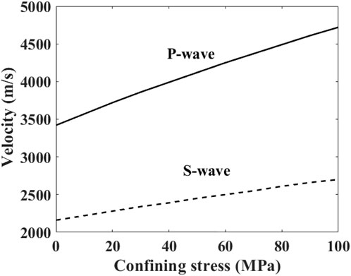
FIGURE 1. Theoretical (exact) velocities values of P-wave and S-wave as a function of confining stress.

FIGURE 2

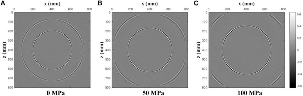
FIGURE 2. Coupled wavefield snapshots of the x-component of the particle velocity at t = 0.1 ms for various confining stresses. ((A): 0 MPa; (B): 50 MPa; (C): 100 MPa)

FIGURE 3

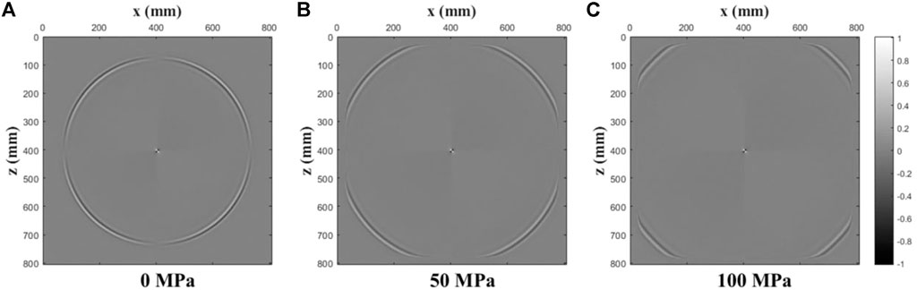
FIGURE 3. Decoupled P-wave field snapshots of the x-component of the particle velocity at t = 0.1 ms for various confining stresses. ((A): 0 MPa; (B): 50 MPa; (C): 100 MPa).

FIGURE 4

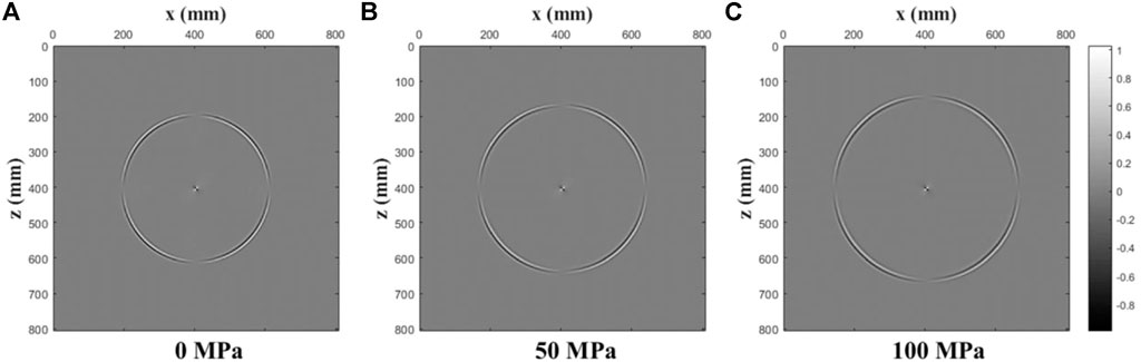
FIGURE 4. Decoupled S-wave field snapshots of the x-component of the particle velocity at t = 0.1 ms for various confining stresses. ((A): 0 MPa; (B): 50 MPa; (C): 100 MPa).

We see that the stress-induced velocity variations are isotropic (circular wavefront), with the amplitude along the wavefront changes in accordance with the characteristics of a vertical force source. Figure 5 shows the single shot records of three wavefields under increasing confining stresses. From the simulation results shown in Figures 2–5, we observe that this scheme can completely separate the pure P-wave and the pure S-wave from the mixed wavefield, thus realizing the decoupling of acoustoelastic wavefield. The simulation results also show that the CPML boundary conditions completely eliminate boundary reflections once the waves hit the border of the model domain, and we only spend 20 grid points to realize this boundary condition. We have to mention that there is a point in the center of the decoupled pure P- and S-wavefield snapshots, because close to the source the elastodynamic wavefield has nearfield terms for which the Helmholtz decomposition does not work (Aki et al., 2002).

FIGURE 5

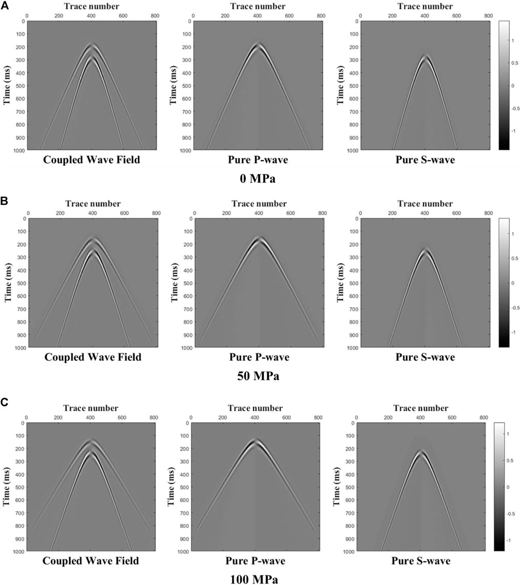
FIGURE 5. Coupled wave field and decoupled P- and S-wave field records of the x-component of the particle velocity for various confining stresses ((A): 0 MPa; (B): 50 MPa; (C): 100 MPa).

In order to verify the correctness of our decoupling, we take a trace (x = 250 mm) from the wavefield snapshot to compare the travel time, amplitude, and phase of the decoupled wavefield and the coupled wavefield. The result is shown in Figure 6. It is not difficult to observe that under different confining pressures, the traveltime, phase and amplitude of the decoupled pure P- and S-wavefield and the coupled wavefield perfectly coincide with each other.

FIGURE 6

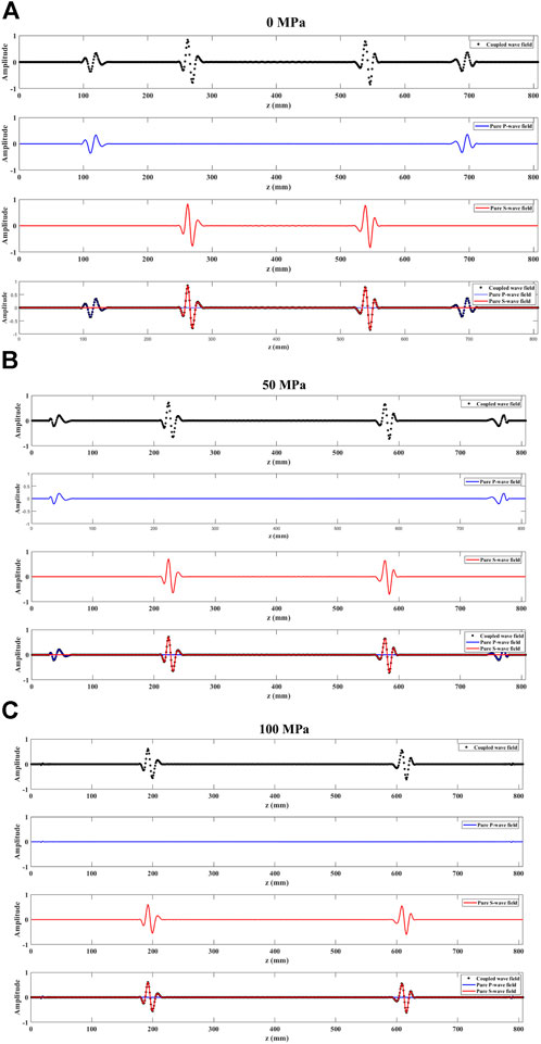
FIGURE 6. Records of x = 250 mm in snapshots above for various confining stresses ((A): 0 MPa; (B): 50 MPa; (C): 100 MPa). (The black dotted lines indicate records of coupled wavefield; the blue solid lines denote records of pure P-wave field; the red solid lines represent records of pure S-wave field). Decoupled acoustoelastic simulation under uniaxial prestress.

Decoupled acoustoelastic simulation under uniaxial prestress

Figures 7, 8 show the wavefield snapshots with increasing uniaxial stresses for the x-component of the particle velocity at t = 0.1 ms. The magnitude of uniaxial prestress can resemble different formation pressures. Figure 7 is the coupled wavefield snapshot, and Figure 8 is a snapshot of the qP-wavefield after decoupling. In Figure 7, with increasing uniaxial stresses, the P- and S-waves are gradually coupled together, with the wavefronts of qP- and qS-waves becoming more elliptical due to the anisotropy of velocities. In Figure 8, we see the decoupled qP-waves, which are roughly the same shape as the qP-waves before decoupling under small stress. However, in the case of high prestress, the two shapes differ from each other. This difference comes from the difference between stress-induced anisotropy and intrinsic anisotropy (Prioul et al., 2004). We also observe shear wave artifacts in the decoupled P-wavefield, but in the context of imaging, these do not seem to cause problems (Duveneck et al., 2008).

FIGURE 7

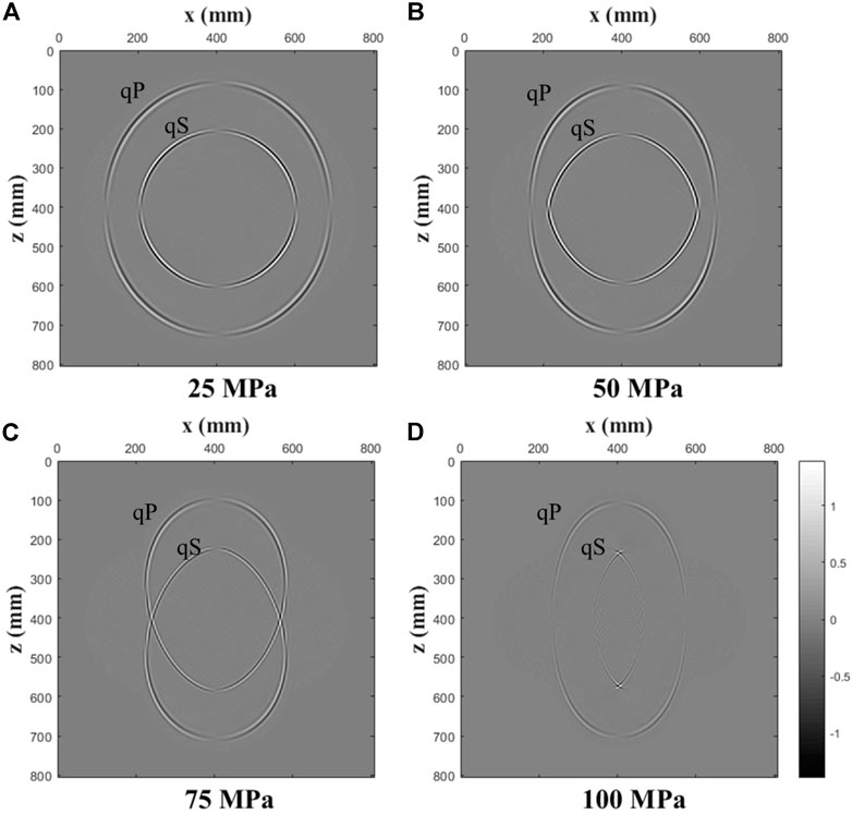
FIGURE 7. Coupled wavefield snapshots of the x-component of the particle velocity at t = 0.1 ms for various uniaxial stresses ((A): 25 MPa; (B): 50 MPa; (C): 75 MPa; (D): 100 MPa).

FIGURE 8

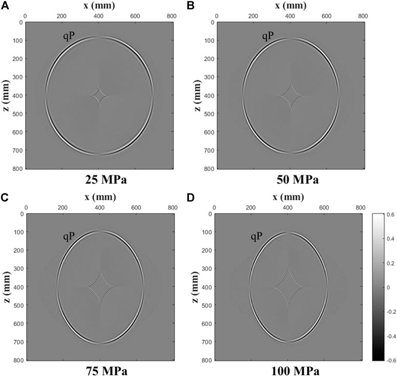
FIGURE 8. Decoupled P-wave field snapshots of the x-component of the particle velocity at t = 0.1 ms for various uniaxial stresses ((A): 25 MPa; (B): 50 MPa; (C): 75 MPa; (D): 100 MPa).

In order to detect the effect of decoupling, we take a trace (x = 350 mm) from the wavefield snapshot to compare the travel time, amplitude, and phase of the decoupled wavefield and the coupled wavefield. The result is shown in Figures 9,10. is a selected part of Figure 9, the red line represents the absolute value of the difference between the two wavefields, and r represents the correlation coefficient between the two wavefields. Obviously, as the uniaxial prestress increases, although the travel times of the qP-waves in the two wavefields fit very well, the amplitude values gradually deviate, that is, the decoupling quality gradually deteriorates. The acoustic approximation is no longer accurate due to the increasingly stronger anisotropic velocity field resulting from the increasing stress-induced anisotropy. But the correlation coefficient of the two curves remains at above 90%, which reflects that this decoupling method is very reliable, even under high anisotropic prestressed conditions.

FIGURE 9

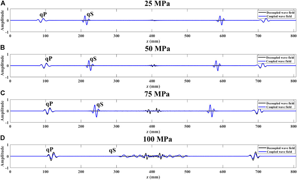
FIGURE 9. Records of x = 350 mm in snapshots above for various uniaxial stresses ((A): 25 MPa; (B): 50 MPa; (C): 75 MPa; (D): 100 MPa). (The black solid lines indicate records of decoupled wavefield; the blue solid lines denote records of coupled wavefield).

FIGURE 10

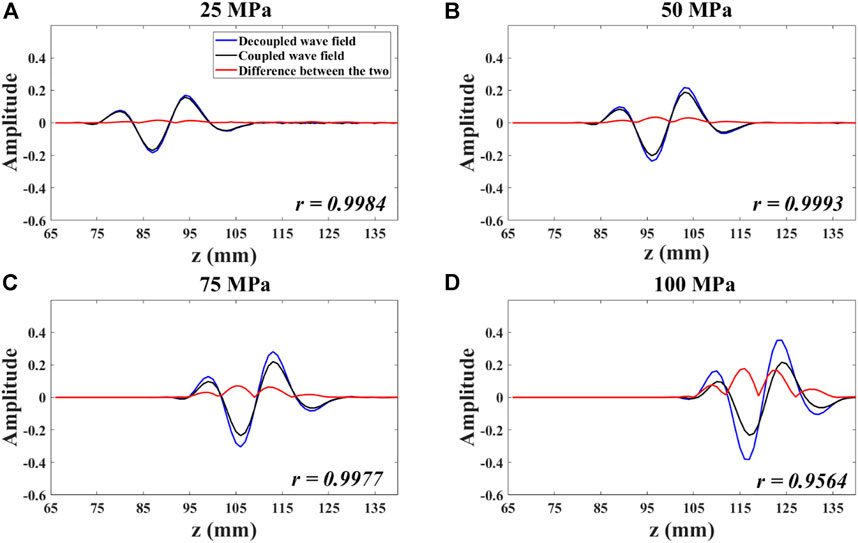
FIGURE 10. Part of Figure 9 ((A): 25 MPa; (B): 50 MPa; (C): 75 MPa; (D): 100 MPa). (Red line represents the absolute value of the difference between the two wavefields; r represents the correlation between the two curves). Decoupled acoustoelastic simulation under the pure shear prestress.

Decoupled acoustoelastic simulation under pure shear prestress

Figures 11, 12 show the coupled and decoupled qP wavefield snapshots with increasing uniaxial stresses for the x-component of the particle velocity at t = 0.1 ms. The magnitude of pure shear pressure corresponds to different geological tension and compression effects. In Figure 11, similar to the case of uniaxial stresses, the wavefronts become more and more elliptical with increasing pure shear stresses. In Figure 12, we also see that as the pressure increases, the diamond-shaped area gradually increases and the decoupling quality gradually deteriorates, similar to the uniaxial case. In order to detect the effect of decoupling, we also take a trace (x = 320 mm) from the wavefield snapshot to compare the travel time, amplitude, and phase of the decoupled wavefield and the coupled wavefield. The result is shown in Figures 13,14 is a selected part of Figure 13.

FIGURE 11

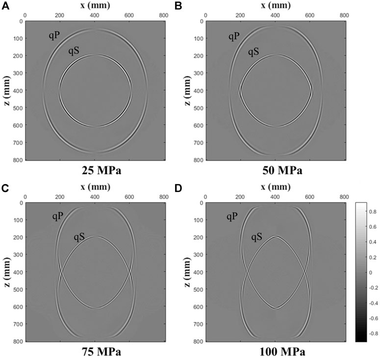
FIGURE 11. Coupled wavefield snapshots of the x-component of the particle velocity at t = 0.1 ms for various pure shear stresses ((A): 25 MPa; (B): 50 MPa; (C): 75 MPa; (D): 100 MPa).

FIGURE 12

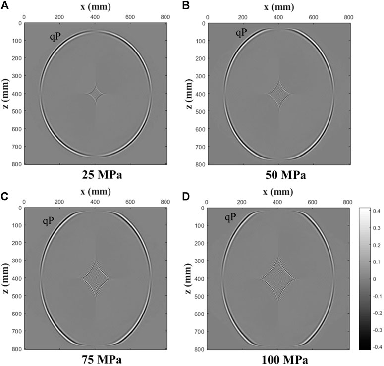
FIGURE 12. Decoupled P-wave field snapshots of the x-component of the particle velocity at t = 0.1 ms for various pure shear stresses ((A): 25 MPa; (B): 50 MPa; (C): 75 MPa; (D): 100 MPa).

FIGURE 13

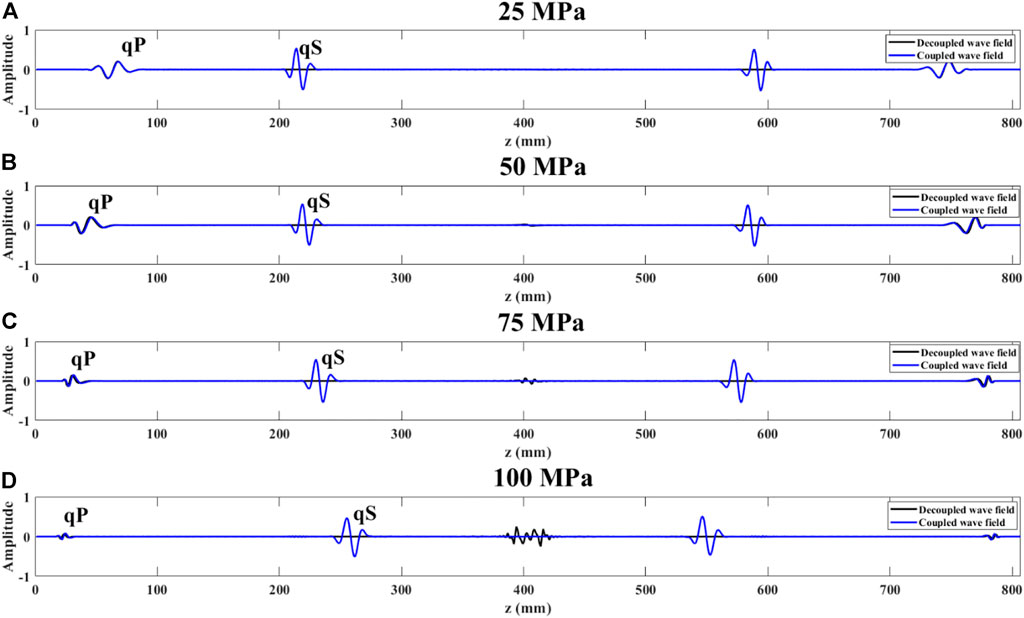
FIGURE 13. Records of x = 320 mm in snapshots above for various pure shear stresses ((A): 25 MPa; (B): 50 MPa; (C): 75 MPa; (D): 100 MPa). (The black solid lines indicate records of decoupled wavefield; the blue solid lines denote records of coupled wavefield).

FIGURE 14

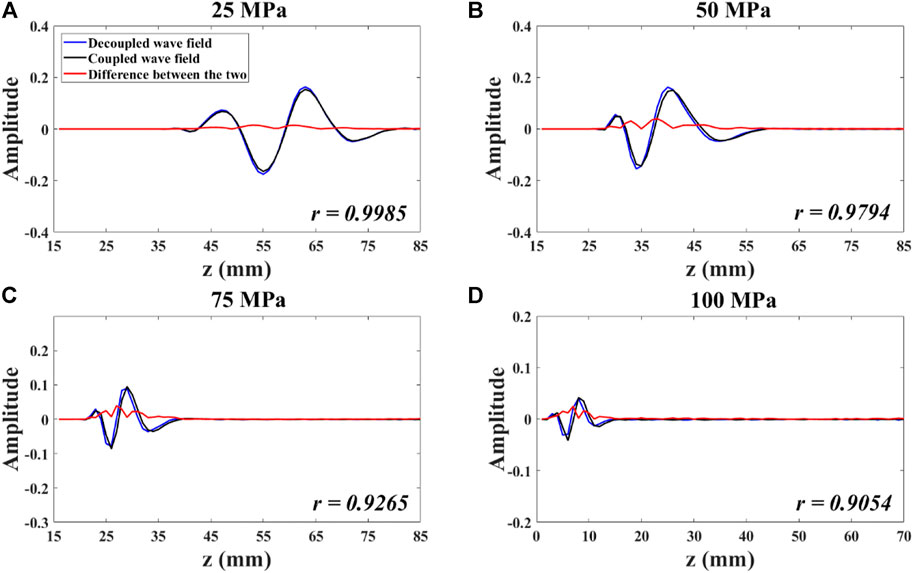
FIGURE 14. Part of Figure 13 ((A): 25 MPa; (B): 50 MPa; (C): 75 MPa; (D): 100 MPa). (Red line represents the absolute value of the difference between the two wavefields; r represents the correlation between the two curves.). Decoupled acoustoelastic simulation for a three-layer model.

Decoupled acoustoelastic simulation for a three-layer model

The three-layer model, separated by a plane interface, is presented to investigate the reflection/transmission at the interface under the three different cases of loading prestress. This model serves as a test for the applicability of the proposed wavefield separation technique in a heterogeneous medium. Figure 15 is the schematic diagram of the three-layer model (900 * 900) mm, the source is at the center of the model. The upper-medium has the same properties as used in the previous simulations. The middle layer has K = 7.5 GPa, μ = 15 GPa, the third-order elastic constants (A, B, C) = (−1,250, −750, −750) GPa, and ρ=2000 kg/m³. The bottom layer has K = 10 GPa, μ = 20 GPa, the third-order elastic constants (A, B, C) = (−1,500, −1,000, −1,000) GPa, and ρ=2000 kg/m³. Consider an interface between two elastic media indicated by the + and − superscripts. The boundary condition at the interface requires the continuity of tractions and displacements. These conditions are written as

$\{\begin{array}{c}{\tau }_{ij}^{+}{n}_j={\tau }_{ij}^{-}{n}_j,\\ u_i^{+}=u_i^{-},\end{array}(41)$

where $n_i$ represents the unit normal to the interface. Einstein’s summation convention for repeating indices is assumed.

FIGURE 15

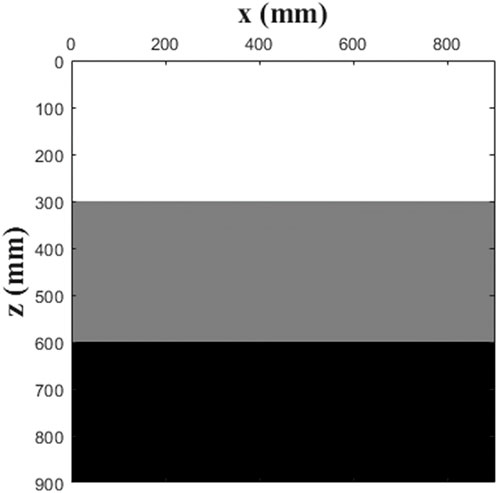
FIGURE 15. Schematic diagram of the three-layer model.

Figures 16–21 show the x-component of the particle velocity snapshots at t = 0.1 ms under three different prestress conditions: confining stress, uniaxial stress, and pure shear stress. All the wave types of reflection/transmission shown in the figure can be observed from these snapshots. This illustrates that the stress-induced velocity anisotropy is strongly related to the orientation of prestresses. The coupled wavefield contains rich information such as direct P waves, PP reflected waves, PS converted waves, and transmitted waves; The P-wavefield separated from the coupled wavefield contains direct P-waves and PP reflections and other longitudinal wave components. Due to the relatively weak amplitude, it is not easy to distinguish various wave phenomena in the mixed wavefield. Through the decoupling of the acoustoelastic wavefield, the transmission and reflection of the P- wave on the interface are made clearer, so we obtain a more concise wave field. This will not only help us understand wave propagation in complex media but also get clearer seismic records in different pre-stressed formations. Other wavefield characteristics are the same as those in the one-layer case, and will not be repeated here.

FIGURE 16

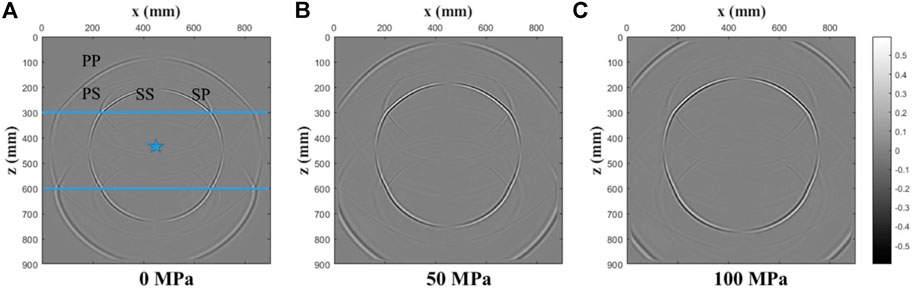
FIGURE 16. Coupled wavefield snapshots of the x-component at t = 0.1 ms for a three-layer model under various confining stresses ((A): 0 MPa; (B): 50 MPa; (C): 100 MPa). The location of the source is marked by a star in the figure. The consecutive wavefronts include P-wave (P), S-wave (S), P-wave transmission (PP), S-wave transmission (SS), S-wave converted by P-wave (PS), and P-wave converted by S-wave (SP).

FIGURE 17

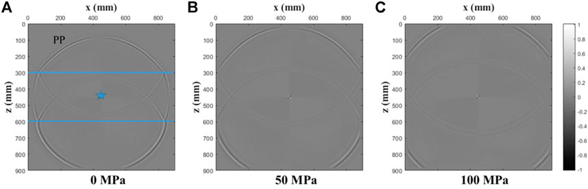
FIGURE 17. Decoupled P-wave field snapshots of the x-component at t = 0.1 ms for a three-layer model under various confining stresses ((A): 0 MPa; (B): 50 MPa; (C): 100 MPa). The location of the source is marked by a star in the figure. The consecutive wavefronts include P-wave (P), and P-wave reflection (PP).

FIGURE 18

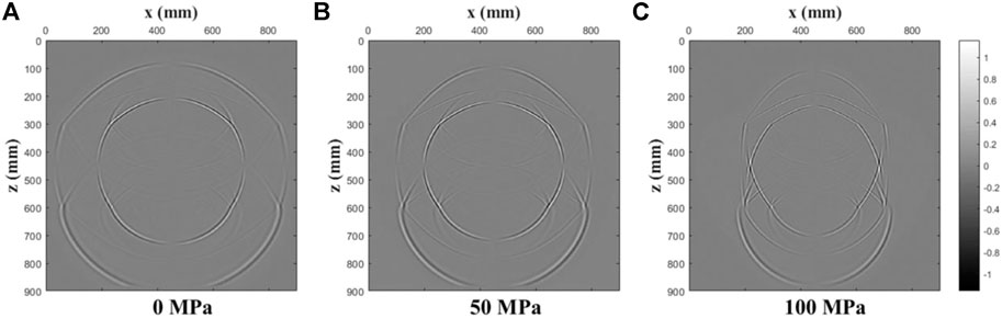
FIGURE 18. Coupled wavefield snapshots of the x-component at t = 0.1 ms for a three-layer model under various uniaxial stresses ((A): 0 MPa; (B): 50 MPa; (C): 100 MPa).

FIGURE 19

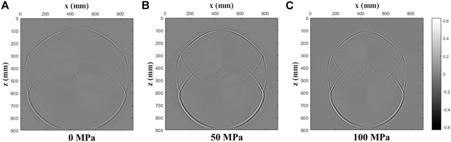
FIGURE 19. Decoupled P-wavefield snapshots of the x-component at t = 0.1 ms for a three-layer model under various uniaxial stresses ((A): 0 MPa; (B): 50 MPa; (C): 100 MPa).

FIGURE 20

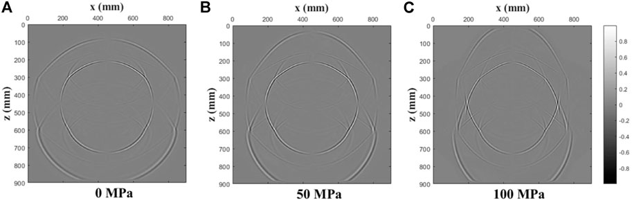
FIGURE 20. Coupled wavefield snapshots of the x-component at t = 0.1 ms for a three-layer model under various pure shear stresses ((A): 0 MPa; (B): 50 MPa; (C): 100 MPa).

FIGURE 21

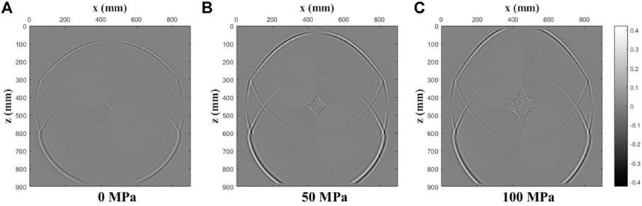
FIGURE 21. Decoupled P-wavefield snapshots of the x-component at t = 0.1 ms for a three-layer model under various pure shear stresses ((A): 0 MPa; (B): 50 MPa; (C): 100 MPa).

Figures 22–24 show the records of x = 300 mm in snapshots for various stresses. Similarly, under confining stress conditions, pressure does not affect the decoupling effect, and the PP waves of the two wavefields match perfectly. However, under uniaxial and pure shear stress fields, prestress will affect the quality of decoupling and will be discussed later.

FIGURE 22

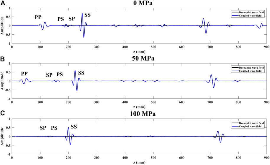
FIGURE 22. Records of x = 300 mm in snapshots above for various confining stresses ((A): 0 MPa; (B): 50 MPa; (C): 100 MPa). (The black solid lines indicate records of decoupled wavefield; the blue solid lines denote records of coupled wavefield).

FIGURE 23

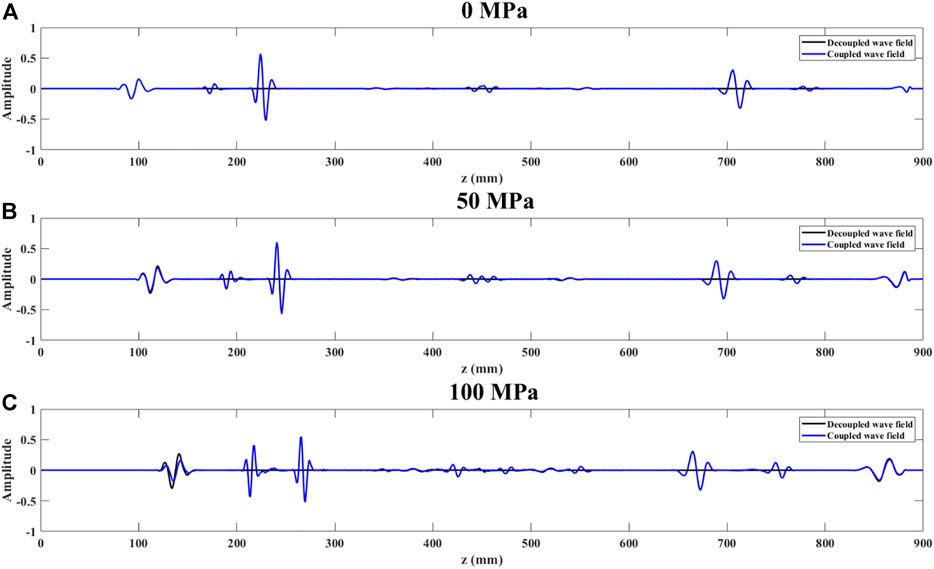
FIGURE 23. Records of x = 300 mm in snapshots above for various uniaxial stresses ((A): 0 MPa; (B): 50 MPa; (C): 100 MPa). (Blue dotted line is a record of coupled wave field; Black line is a record of decoupled P-wave field).

FIGURE 24

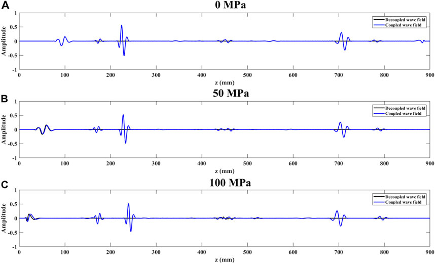
FIGURE 24. Records of x = 300 mm in snapshots above for various pure shear stresses ((A): 0 MPa; (B): 50 MPa; (C): 100 MPa). (Blue dotted line is a record of coupled wave field; Black line is a record of decoupled P-wave field.

Discussion

The decoupling scheme under anisotropic prestresses is formulated by applying the acoustic approximation (Duveneck et al., 2008) to acoustoelasticity equations. From the comparison of coupled and decoupled wavefields in traveltime and amplitude, the scheme is reliable even under the strong anisotropic prestress. There exists a diamond-shaped area in the center of the modeling domain where the source is located. As discussed, e.g., by Grechka et al. (2004), this is a well-known problem of source-generated shear waves which are regarded as artifacts for P-wave modeling. These qS-wave artifacts are usually suppressed, for example, by placing the source in the isotropic part of the model (Duveneck et al., 2008). Alternatively, we can partly eliminate artifacts in numerical simulations by assuming no prestress around the source to make the near-source region isotropic.

Stress-induced anisotropy depends largely on anisotropic prestress loading (Sinha and Kostek, 1996). As indicated by Alkhalifah (2000), the kinematic error of decoupling becomes larger as the anisotropy increases, implying that the decoupling becomes worse. This is why anisotropic prestresses affect the accuracy of decoupling approximations. However, for the acoustoelasticity decoupling, this error appears mainly in amplitude based on the numerical simulations presented in this study. Intrinsic anisotropies in rocks generally result from the alignment of grains and microstructures making up the rock matrix. Particularly, prestress causes the “closure” of microcracks (Sayers, 2002), inducing preferred orientation that makes rocks anisotropic. Knowledge of stress-induced anisotropy can predict the distribution of wave velocities in formations as accurately as possible. Therefore, the introduction of stress-dependent anisotropy into wave equations can give an efficient modeling strategy. It has important implications for seismic AVO and geomechanical applications.

Conclusion

The theory of acoustoelasticity results from the third-order elasticity with a cubic term of the strain energy function. It describes wave propagation in prestressed media by relating wave velocities to prestresses. We formulate the first-order velocity-stress decoupled acoustoelasticity equations that are solved by the RSG-FD numerical method with the CPML absorbing boundary. Numerical simulations are conducted for a homogeneous medim and a triple-layer model, respectively, under three typical states of confining, uniaxial, and pure-shear prestress conditions. We investigate the effect of prestress conditions on the decoupling accuracy.

Numerical examples show that the proposed decoupling scheme yields a good kinematic P-wave approximation to the acoustoelasticity equations, implying its potential applications in seismic imaging and inversion under prestress conditions. Under the confining pressure, the acoustoelasticity equations can be decopled into pure P- and S-wave equations through the Helmholtz decomposition, resulting in a complete separation of longitudinal and transverse wavefields in both amplitude and traveltime. Under the anisotropic prestress conditions (uniaxial and pure-shear), the decoupled and coupled wavefields match well in amplitude and traveltime at low pressures. However, when the pressure is too high, we see certain deviations in amplitude and phase, but the decoupling accuracy is still reliable because of the high correlation coefficient of these two wavefields. We also observe shear wave artifacts in the decoupled P wavefield. For a three-layer model under the same prestress conditions, the decoupled P wavefield includes direct, reflected, and transmitted P waves only, where various converted S waves are removed.

Data availability statement

The original contributions presented in the study are included in the article/Supplementary Material, further inquiries can be directed to the corresponding author.

Author contributions

L-YF and HY conceive this research. HY writes the manuscript and prepares the figures. L-YF and B-YF reviews and supervises the manuscript. The coauthors TM are involved in the discussion of the manuscript. All authors finally approve the manuscript and thus agree to be accountable for this work.

Funding

The research was supported by the National Natural Science Foundation of China (Grant No. 41821002) and 111 Project “Deep-Superdeep Oil & Gas Geophysical Exploration” (B18055).

Conflict of interest

The authors declare that the research was conducted in the absence of any commercial or financial relationships that could be construed as a potential conflict of interest.

The handling editor JDDB declared a past co-authorship with the author TMM.

Publisher’s note

All claims expressed in this article are solely those of the authors and do not necessarily represent those of their affiliated organizations, or those of the publisher, the editors and the reviewers. Any product that may be evaluated in this article, or claim that may be made by its manufacturer, is not guaranteed or endorsed by the publisher.

Supplementary Material

The Supplementary Material for this article can be found online at: https://www.frontiersin.org/articles/10.3389/feart.2022.1031490/full#supplementary-material

References

Aki, K., and Richards, P. G. (2002). Quantitative seismology.

Google Scholar

Alkhalifah, T. (1998). Acoustic approximations for processing in transversely isotropic media. Geophysics 63 (2), 623–631. doi:10.1190/1.1444361

CrossRef Full Text | Google Scholar

Alkhalifah, T. (2000). An acoustic wave equation for anisotropic media. Geophysics 65 (4), 1239–1250. doi:10.1190/1.1444815

CrossRef Full Text | Google Scholar

Alkhalifah, T. (2003). An acoustic wave equation for orthorhombic anisotropy. Geophysics 68 (4), 1169–1172. doi:10.1190/1.1598109

CrossRef Full Text | Google Scholar

Carcione, J. M. (1999). Staggered mesh for the anisotropic and viscoelastic wave equation. Geophysics 64 (6), 1863–1866. doi:10.1190/1.1444692

CrossRef Full Text | Google Scholar

Carcione, J. M., Wang, W., Ling, E., Salusti, J., Ba, L., and Fu, Y. (2019). Simulation of wave propagation in linear thermoelastic media. Geophysics 84 (1), T1–T11. doi:10.1190/geo2018-0448.1

CrossRef Full Text | Google Scholar

Carcione, J. M. (2007). Wave fields in real media: Wave propagation in anisotropic, anelastic, porous and electromagnetic media. Elsevier.

Google Scholar

Chang, W. F., and McMechan, G. A. (1986). Reverse-time migration of offset vertical seismic profiling data using the excitation-time imaging condition. Geophysics 51 (1), 67–84. doi:10.1190/1.1442041

CrossRef Full Text | Google Scholar

Dellinger, J., and Etgen, J. (1990). Wave-field separation in two-dimensional anisotropic media. Geophysics 55 (7), 914–919. doi:10.1190/1.1442906

CrossRef Full Text | Google Scholar

Du, X., Fletcher, R. P., and Fowler, P. J. (2008). “A new pseudo-acoustic wave equation for VTI media,” in 70th EAGE conference and exhibition incorporating SPE EUROPEC 2008 (Rome: European Association of Geoscientists & Engineers), 40.

CrossRef Full Text | Google Scholar

Duveneck, E., Milcik, P., Bakker, P. M., and Perkins, C. (2008). “Acoustic VTI wave equations and their application for anisotropic reverse-time migration,” in SEG technical program expanded abstracts 2008 (Las Vegas, Nevada: Society of Exploration Geophysicists), 2186–2190.

Google Scholar

Fowler, P. J., Du, X., and Fletcher, R. P. (2010). Coupled equations for reverse time migration in transversely isotropic media. Geophysics 75 (1), S11–S22. doi:10.1190/1.3294572

CrossRef Full Text | Google Scholar

Goldberg, Z. A. (1961). Interaction of plane longitudinal and transverse elastic waves. Sov. Phys. Acoust. 6, 306–310.

Google Scholar

Grechka, V., Zhang, L., and Rector, J. W. (2004). Shear waves in acoustic anisotropic media. Geophysics 69 (2), 576–582. doi:10.1190/1.1707077

CrossRef Full Text | Google Scholar

Green, R. E. (1973). Treatise on Materials Science and Technology, 3. New York: Academic Press.Ultrasonic investigation of mechanical properties.

Google Scholar

Huang, X., Burns, D. R., and Toksöz, M. N. (2001). The effect of stresses on the sound velocity in rocks: Theory of acoustoelasticity and experimental measurements. Tech. Report. Boston: Earth Resources Laboratory, Massachusetts Institute of Technology.

Google Scholar

Igel, H., Mora, P., and Riollet, B. (1995). Anisotropic wave propagation through finite-difference grids. Geophysics 60 (4), 1203–1216. doi:10.1190/1.1443849

CrossRef Full Text | Google Scholar

Johnson, P. A., and Shankland, T. J. (1989). Nonlinear generation of elastic waves in granite and sandstone: Continuous wave and travel time observations. J. Geophys. Res. 94, 17729–17733. doi:10.1029/jb094ib12p17729

CrossRef Full Text | Google Scholar

Kindelan, M., Kamel, A., and Sguazzero, P. (1990). On the construction and efficiency of staggered numerical differentiators for the wave equation. Geophysics 55 (1), 107–110. doi:10.1190/1.1442763

CrossRef Full Text | Google Scholar

Komatitsch, D., and Martin, R. (2007). An unsplit convolutional perfectly matched layer improved at grazing incidence for the seismic wave equation. Geophysics 72 (5), SM155–SM167. doi:10.1190/1.2757586

CrossRef Full Text | Google Scholar

Martin, R., and Komatitsch, D. (2009). An unsplit convolutional perfectly matched layer technique improved at grazing incidence for the viscoelastic wave equation. Geophys. J. Int. 179 (1), 333–344. doi:10.1111/j.1365-246x.2009.04278.x

CrossRef Full Text | Google Scholar

Meegan, G. D., Johnson, R. A., Guyer, P. A., and McCall, K. R. (1993). Observations of nonlinear elastic wave behavior in sandstone. J. Acoust. Soc. Am. 94, 3387–3391. doi:10.1121/1.407191

CrossRef Full Text | Google Scholar

Pao, Y.-H., Sachse, W., and Fukuoka, H. (1984). “Acoustoelasticity and ultrasonic measurements of residual stresses,” in Physical acoustics, principles and methods. Editors W. P. Mason,, and R. N. Thurston (Orlando: Academic Press), 61–143.

Google Scholar

Pao, Y. H., and Gamer, U. (1985). Acoustoelastic waves in orthotropic media. J. Acoust. Soc. Am. 77 (3), 806–812. doi:10.1121/1.392384

CrossRef Full Text | Google Scholar

Prioul, R., Bakulin, A., and Bakulin, V. (2004). Nonlinear rock physics model for estimation of 3D subsurface stress in anisotropic formations: Theory and laboratory verification. Geophysics 69 (2), 415–425. doi:10.1190/1.1707061

CrossRef Full Text | Google Scholar

Pugin, A., and Yilmaz, Ö. (2019). Optimum source-receiver orientations to capture PP, PS, SP, and SS reflected wave modes. Lead. Edge 38 (1), 45–52. doi:10.1190/tle38010045.1

CrossRef Full Text | Google Scholar

Saenger, E. H., Gold, N., and Shapiro, S. A. (2000). Modeling the propagation of elastic waves using a modified finite-difference grid. Wave motion 31 (1), 77–92. doi:10.1016/s0165-2125(99)00023-2

CrossRef Full Text | Google Scholar

Saenger, E. H., and Shapiro, S. A. (2002). Effective velocities in fractured media: A numerical study using the rotated staggered finite-difference grid. Geophys. Prospect. 50 (2), 183–194. doi:10.1046/j.1365-2478.2002.00309.x

CrossRef Full Text | Google Scholar

Sayers, C. M. (2002). Stress-dependent elastic anisotropy of sandstones. Geophys. Prospect. 50, 85–95. doi:10.1046/j.1365-2478.2002.00289.x

CrossRef Full Text | Google Scholar

Sinha, B. K., and Kostek, S. (1996). Stress-induced azimuthal anisotropy in borehole flexural waves. Geophysics 61, 1899–1907. doi:10.1190/1.1444105

CrossRef Full Text | Google Scholar

Sun, R., and McMechan, G. A. (2001). Scalar reverse-time depth migration of prestack elastic seismic data. Geophysics 66 (5), 1519–1527. doi:10.1190/1.1487098

CrossRef Full Text | Google Scholar

Sun, R., McMechan, H. H., Hsiao, G. A., and Chow, J. (2004). Separating P-and S-waves in prestack 3D elastic seismograms using divergence and curl. Geophysics 69 (1), 286–297. doi:10.1190/1.1649396

CrossRef Full Text | Google Scholar

Thomsen, L. (1986). Weak elastic anisotropy. Geophysics 51 (10), 1954–1966. doi:10.1190/1.1442051

CrossRef Full Text | Google Scholar

Virieux, J. (1986). P-SV wave propagation in heterogeneous media: Velocity-stress finite-difference method. Geophysics 51 (4), 889–901. doi:10.1190/1.1442147

CrossRef Full Text | Google Scholar

Winkler, K. W., and Liu, X. (1996). Measurements of third-order elastic constants in rocks. J. Acoust. Soc. Am. 100 (3), 1392–1398. doi:10.1121/1.415986

CrossRef Full Text | Google Scholar

Yan, J., and Sava, P. (2008). Isotropic angle-domain elastic reverse-time migration. Geophysics 73 (6), S229–S239. doi:10.1190/1.2981241

CrossRef Full Text | Google Scholar

Zharnikov, T., Ponomarenko, R., Nikitin, A., and Ayadiuno, C. (2022). “Analysis of the effect of geomechanical stress on the acoustic response of anisotropic rocks,” in International Petroleum technology conference (Riyadh, Saudi Arabia: OnePetro).

CrossRef Full Text | Google Scholar

Zhou, H., Zhang, G., and Bloor, R. (2006). “An anisotropic acoustic wave equation for modeling and migration in 2D TTI media,” in SEG technical program expanded abstracts 2006 (New Orleans: Society of Exploration Geophysicists), 194–198.

CrossRef Full Text | Google Scholar

Zuo, P., Liu, Y., and Fan, Z. (2022). Modeling of acoustoelastic borehole waves subjected to tectonic stress with formation anisotropy and borehole deviation. Geophysics 87 (1), D1–D19. doi:10.1190/geo2020-0859.1

CrossRef Full Text | Google Scholar