Fast imaging for the 3D density structures by machine learning approach

Residual Bouguer gravity anomaly inversion can be used to imaging for local density structures or to interpret near-surface anomalous mass distribution. The reasonable prior information is the crucial recipe for obtaining a realistic geological inversion result, especially for the ill-posed geophysical inversion problem. The conventional strategies introduce the prior constraints or joint multidisciplinary information in object function as regularization, and then use some optimization algorithm to minimize the object function. This process is called model-driven approach and is usually time-consuming. In recent years, the rapid development of machine learning technology has provided new solutions for solving geophysical inversion problems. Machine learning methods can reduce the dependence on prior information in the inversion process through setting special training datasets, and the time consumption of an inversion process executed by the trained model can be shortened by several orders of magnitude, which is conducive to fast inversion for the same type of application scenarios. In this study, we were inspired by the U-net model and develops the GV-Net (Gravity voxels inversion network) model using the convolutional neural network for the inversion of residual gravity anomalies. We first discussed the effects of different loss functions on the convergence speed of model training and prediction accuracy. Then, we analyzed the robustness of our model by changing noise levels of the datasets. At last, we employed this model in a real scenario. The results have demonstrated that the GV-Net model has the ability to deal with specific inverse problems by predefined training datasets.

1 Introduction

Gravity method as one of multidisciplinary geophysics methods is sensitive to density distribution, which can be used to imaging for the density structure of the shallow Earth (Wang et al., 2014; Honglei et al., 2021). In general, different sort of gravity anomaly exist their own special geophysical meaning (Johannes and Smilde, 2009). The Bouguer gravity anomaly can be divided into regional and residual parts according to the characteristics of the field sources. The regional Bouguer gravity anomalies are controlled by large-scale structural anomalies or deep density anomalies, such as Moho depth (Fu et al., 2014) and basement relief. The residual Bouguer gravity anomaly, also known as local gravity anomaly, correspondence to the distribution of residual mass in the shallow crust. Generally, the residual Bouguer gravity anomaly can be used in the mineral exploration or the near-surface geological structure detection (Rosid et al., 2020; Chen and Zhang, 2022).

Gravity inversion is a necessary procedure for retrieving geological information from gravity anomalies. However, similar to other geophysical inversion problems, gravity inversion problem is usually ill-posed and the result is inherent non-unique. For the same gravity anomaly, infinite mathematical solutions can be found for fitting the input anomaly within a certain tolerance. Therefore, geoscientists usually introduce certain prior information to constrain the inversion process for obtaining a reasonable outcome, such as minima structure constraint, smoothness assumption (Li and Oldenburg, 1996; Li and Oldenburg, 1998), and so on. Nevertheless, how to select the prior constraints are generally limited by researchers’ experience, and improper prior constrains will inevitably introduce spurious features into the inversion results. The joint inversion with multidisciplinary geophysical data is an effective approach to reducing the non-uniqueness of inversion results (Bosch et al., 2006; Lelièvre et al., 2012; Liu et al., 2022). But this approach relies on the relationships between different physical properties, these are also empirical and not suitable for all geological conditions. Additionally, in traditional inversion strategies, the large-scale systems of linear or non-linear equations must be solved whatever using the direct or iterative method. Especially for regularized inversion method, the ‘trade-off’ parameter is often obtained through multiple iterations, this process is time-consuming.

Recent development of machine learning (ML) technique brings a new strategy for scientists to solve tough problems. ML term first appeared in literature can be traced to the 1950s (Turing, 1950). Nevertheless, due to the limitation of computer performance and the high requirement of mathematical ability for researchers, ML has not received much attention for a long time. In the past decade, computer performance has developed rapidly, especially with the emergence of general ML frameworks such as TensorFlow, PyTorch, MXNet, Keras, and Theano. Kinds of ML frameworks make us deploy and train the ML models simply and efficiently. At the same time, the powerful GPU continually enhances the training efficiency of complex ML model and makes it feasible to deal with high dimensionality problems with a large-scale degree of freedom. ML approach has already shown extraordinary potential and for solving the geophysical inversion problems in numerous geoscience scenarios.

ML is a sort of data-driven method, which has been widely used in geosciences, including seismology (Kong et al., 2018; Ming et al., 2019a; Ming et al., 2019b), solid Earth geoscience (Bergen et al., 2019), hydro-geophysics (Shen, 2018), geomorphometry (Valentine and Kalnins, 2016) and sea ice forecasting (Andersson et al., 2021). In this study, we introduce ML to imaging the 3D density structure in the shallow crust. For the 3D gravity inverse problem, the input data can be regarded as a single-channel image, and the output can be assumed as multi-channel images, so this problem can be applied with CNN(Convolutional Neural Network), which is a typical ML method.

During the training process, the model updates the parameters according to the pre-defined loss function to fitting the mapping relationship between the observed data and the field source parameters. The well-trained ML model transforms the conventional inverse problem into a forward problem, which greatly shortens the time required for model prediction. In this study, we first proposed the GV-Net model inspired by U-Net (Ronneberger et al., 2015) for the 3D density structure imaging. Then we generated a large number of model-observation data samples by a random algorithm as training datasets artificially. Subsequently, we test the influence of two different loss functions with respect to the model training speed, model convergence characteristics, and model prediction accuracy. At last, we verified that the GV-net model is noise resistant, and we also demonstrated the practicality of the GV-net model through a real scenario.

2 Methodology

2.1 The architecture of GV-Net

In this study, we developed the GV-Net model based on CNN technology. Figure 1 illustrates the architecture of the GV-Net model, which is primarily composed of four components, namely preprocessing, encoder, decoder, and output respectively. The activation function uses the Relu function, and the pooling method is maximum pooling. The detailed procedure of the GV-Net model is illustrated in Table 1. We use PyTorch framework to construct and train the GV-Net model.

FIGURE 1

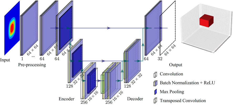
FIGURE 1. Schematic of GV-Net architecture.

TABLE 1

TABLE 1. The algorithm of GV-Net.

The input data of GV-Net is a single-channel image with 64 × 64 pixels, each pixel represents a gravity data point. Then, we gradually increased the number of channels to 64 through the preprocessing part, with the horizontal resolution of the data in the preprocessing part remains unchanged. The horizontal resolution of the data is then reduced to 8×8 in the encoder part by three Max-pooling processes, while the number of channels is increased to 512. In the decoder part, the number of channels of the model is reduced to 64 by three transposed convolution operations, and the resolution will be increased to 64×64. Finally, the output part generates the 32 channels, which have 64×64 data points in each channel to express the density voxel layers in the three-dimensional space implemented by a convolution layer.

2.2 Loss function

During the CNN training, the model parameters will be updated according to the variation of the loss function. Therefore, selecting a suitable loss function is critical for improving the model performance. We chose two sorts of loss functions as candidates to test the effect on the GV-Net model, including training speed, convergence characteristics, and prediction accuracy.

1) Mean squared Error (MSE) function

Mean squared error (MSE) is one of the most common loss functions used in machine learning, which has been widely adopted in regression problems (Mitra et al., 2020; Wang et al., 2020; He et al., 2021). MSE_Loss function can be expressed as

$MS{E}_{\mathrm{L}\mathrm{o}\mathrm{s}\mathrm{s}\left(\widehat{m},m\right)}=\frac{1}{N}{\displaystyle \sum }_{i=1}^N{\left({\widehat{m}}_i-m_i\right)}^2(1)$

where $m$ is the true model, $\widehat{m}$ is the predicted model, $N$ is number of elements in model $m$

2) Dice function

Milletari et al. (2016) proposed a loss function based on Dice coefficient to measure the similarity of two models. The dice coefficient can be written as

$Dice\left(\widehat{m},m\right)=\frac{2{\displaystyle \sum }_{i=1}^N{\widehat{m}}_i{m}_i}{{\displaystyle \sum }_{i=1}^N{\widehat{m}}_i^2+{\displaystyle \sum }_{i=1}^N{m}_i^2}(2)$

Then, the Dice function can be expressed as

$Dic{e}_{Loss\left(\widehat{m},m\right)}=1-Dice\left(\widehat{m},m\right)(3)$

Based on Eq. 2, when the predicted model is closer to the real model, the Dice coefficient is closer to one, which makes the $Dic{e}_{Loss}$ closer to zero. Huang et al. (2021) use this loss function to deal with sparsity inversion problems with binary density distribution and got good results.

In the following sections, we refer to the GV-Net with MSE_Loss function as MGV-Net and refer to the GV-Net with Dice_Loss function as DGV-Net.

2.3 Result evaluation metrics

For evaluating the prediction accuracy of GV-Net and comparing the effect of two different loss functions, we introduce two metrics to quantitatively evaluate the predicted result from different aspects. The first metric is called model relative error ε, which can be used to evaluate the predicted density source, and this metric is expressed as follows:

$\epsilon =\frac{{‖\widehat{m}-m‖}_2}{{‖\widehat{m}‖}_2+{‖m‖}_2}(4)$

This metric function is range from 0 to 1, as shows in Eq. 4, which means the more accurate the model predicts, the smaller ε is.

The second metric index is to assess the gravity anomaly generated by the predicted density model. We introduce the mean squared of data misfit to express how the recovered gravity fits the true gravity anomaly in each prediction, which shows in Eq. 5.

$\overline{\omega }=\frac{1}{N}{\displaystyle \sum }_{i=1}^N{\left({\overline{d}}_i-d_i\right)}^2(5)$

where N is the number of gravity anomaly data, $d_i$ is the ith true gravity anomaly, ${\overline{d}}_i$ is the ith predicted gravity.

3 Training datasets

3.1 Voxel modeling

In geophysical research, it is necessary to modeling the research object and then parameterization the characteristics of the geophysical field source through a number of models. In gravity field inversion, we generally use a series of regular bodies to approximate the field source model for different research problems, and each regular body has a specific density. Common regular density models include sphere model, cylinder model, and rectangular prism model.

In this study, to describe the characteristics of the stochastic distribution of density contrast flexibly, we simulated the subsurface structure with regularly arranged rectangle prism cells according to a certain grid spacing, and the gravity data are measured from fixed ground observation points. The density model and the observing system illustrated in Figure 2. Borrowing the term pixel in two-dimensional images, we refer to each density prism in three-dimensional space as a voxel. The relationship between the gravity anomaly and the density voxels can be expressed as:

$\left[\begin{array}{c}{d}_1\\ d_2\\ d_3\\ ⋮\\ d_N\end{array}\right]=\left[\begin{array}{ccc}\begin{array}{ccc}{\gamma }_{\mathrm{1,1}}& {\gamma }_{\mathrm{1,2}}& {\gamma }_{\mathrm{1,3}}\\ {\gamma }_{\mathrm{2,1}}& {\gamma }_{\mathrm{2,2}}& {\gamma }_{\mathrm{2,3}}\\ {\gamma }_{\mathrm{3,1}}& {\gamma }_{\mathrm{3,2}}& {\gamma }_{\mathrm{3,3}}\end{array}& \cdots & \begin{array}{c}{\gamma }_{1,M}\\ {\gamma }_{2,M}\\ {\gamma }_{3,M}\end{array}\\ ⋮& \ddots & ⋮\\ \begin{array}{ccc}{\gamma }_{N,1}& {\gamma }_{N,2}& {\gamma }_{N,3}\end{array}& \cdots & {\gamma }_{N,M}\end{array}\right]\left[\begin{array}{c}{m}_1\\ m_2\\ m_3\\ ⋮\\ m_M\end{array}\right](6)$

where $d_i$ is the gravity datum at $i$ th observation station, $m_j$ is the density contrast of $j$ th prism, ${\gamma }_{i,j}$ is the kernel operator, N is the number of observation points, and M is the number of voxels.

FIGURE 2

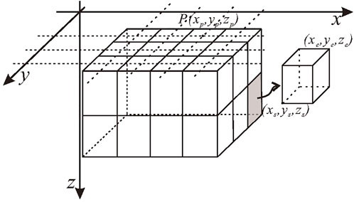
FIGURE 2. Schematic diagram for the gravity anomaly of discretized prism models.

The kernel operator is defined by the volume of the voxel, density contrast, the location of observation points, and the position of the voxel. The kernel operator ${\gamma }_{i,j}$ can be expressed as follows:

${\gamma }_{i,j}=G{\int }_{z_s}^{z_e}{\int }_{y_s}^{y_e}{\int }_{x_s}^{x_e}\frac{∆\rho \left(z_p-z\right)}{r^3}dxdydz(7)$

where $G=6.67\times {10}^{-1}N\cdot m^2\cdot k{g}^{-2}$ is the gravitational constant, x, y, z are coordinates of the density body in the three directions respectively, $r=\sqrt{{\left(x_p-x\right)}^2+{\left(y_p-y\right)}^2+{\left(z_p-z\right)}^2}$ represent the distance from the field source to the observed position. While the density is constant, which mean $∆\rho ={\rho }_c$, Eq. 7 becomes (Nagy et al., 2000):

${\gamma }_{i,j}={\rho }_{c}G|||\left(x_p-x\right)\ln \left[\left(y_p-y\right)+r\right]+y\ln \left[\left(x_p-x\right)+r\right]-z{\tan }^{-1}\frac{\left(x_p-x\right)\left(y_p-y\right)}{\left(z_p-z\right)r}{|}_{x_s}^{x_e}{|}_{y_s}^{y_e}{|}_{y_s}^{y_e}(8)$

3.2 Datasets generation

The ML model training is necessary to utilize large enough labeled datasets. Because the conventional Green’s function between the gravity response and field source cannot be directly transformed to the weight values of the designed CNN model. In the training process, an abundant training dataset needs to be used to build the mapping relationship between the input and output. The features of the training datasets directly determine the application scenarios of the model. In this study, we trained the GV-net model with plenty of voxels by the presupposed prior density assumption as the output of the GV-Net and calculated the corresponding gravity anomaly at the observed grid as the input of the GV-Net. The input gravity anomaly was the superposition of all voxel anomalies in one field source. If repeated this generation time by time, the location of a voxel in the field source model is stochastic for simulating various density distribution situations as much as possible.

Figure 3 shows four randomly generated density models. The models are composed of rectangle prisms of different scales and arrangements, so theoretically, they can approximately represent the distribution of density anomalies with different shapes. In this study, the size of each voxel is 50 m×100 m×100 m, and the density contrast of each block is .5–1.0 g/cm³. A total of 19,200 sets of data are used for training and 2,000 sets of data were used for validation for both DGV-Net and MGV-Net.

FIGURE 3

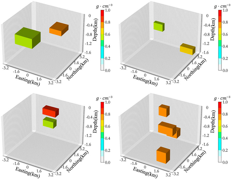
FIGURE 3. Examples of random density model.

4 Result

4.1 Model training

Figure 4 shows the loss function and model relative error of DGV-Net and MGV-Net, respectively. To reduce time costs and ensure the stability of the loss curves and error curves, the loss value and error on curves are calculated by the prediction results of 200 random samples from relevant datasets, rather than all datasets.

FIGURE 4

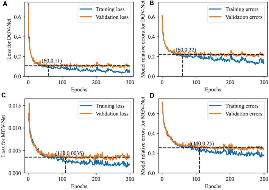
FIGURE 4. Loss curves and model relative errors for the training and validation datasets.

During the training of DGV-Net and MGV-Net, both the loss curves and error curves decreased smoothly with the increase of epochs, but there are a few different behaviors between training datasets and validation datasets. The curves associated with validation datasets (Orange curves) tend to be stable when the epochs reach a certain value, while the curves associated with training datasets (Blue curves) are not stable until the end of epochs. These features illustrated that for a random model, which are most likely not in the training datasets, the GV-Net predicts accuracy restricted to a level because of using the finite training datasets.

Moreover, the validation loss curve of DGV-Net reaches to a steady state faster than MGV-Net, which means the Dice loss is more conducive to the convergence of the GV-Net model.

The model relative error curves in Figure 3 and Figure 3 show that the prediction accuracy of DGV-Net is better than MGV-Net. Therefore, we can estimate that DGV-Net will have better performance than MGV-Net for anomalous models that are not in the training datasets.

Table 2 shows the time required for GV-Net training process and single prediction. We can see that the training time when employing the root mean square loss function is significantly less than that using the Dice loss function. The time required for single prediction using the trained model is far less than 1s. Consequently, when the GV-Net is used for inversion problems, as long as the model is well-trained, fast inversion can be executed for the same type of problems. Comparison with other research for fast inversion solutions, such as compressive inversion (Foks et al., 2014), and adaptive mesh inversion (Davis and Li, 2011). Our approach reflects sufficient efficiency.

TABLE 2

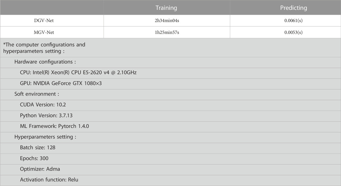
TABLE 2. Time cost.

4.2 Model validation

In order to illustrate the inversion effect of GV-Net more intuitively, we designed three typical density models to evaluate the performance of GV-Net with two different loss functions. The three models were the horizontal distributed density model, the dipping dyke density model, and the vertical distributed density model respectively. The residual density and model grid setting are consistent with the training datasets. To clearly show the shape of the retrieved model, only the voxels with a density greater than or equal to 0.3 g/cm³ are drawn for the results in the following figures.

1) Horizontal distributed density model

Generally, gravity is sensitive to the lateral variations of the density contrast, so we designed a model with two density blocks that are totally separate in horizontal (Figure 5A) to test the ability of GV-Net to identify lateral density variations. The gravity response of this model (Figure 5B) sharply depicts the contour of this model in the horizontal direction. The results (Figures 5C, D) demonstrated that both DGV-Net and MGV-Net can predict the outcome with reasonable accuracy for the density contrast with horizontal distribution characteristics.

FIGURE 5

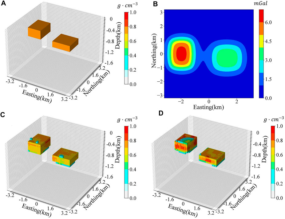
FIGURE 5. Horizontal distributed density model (A) The shape of the horizontal distributed density model; (B) Gravity anomalies that correspond to the true model; (C) The model recovered by DGV-Net; (D) The model recovered by MGV-Net.

Figure 6 shows the forward gravity and gravity misfit from predicted density contrast. The max misfit in recovered gravity is less than 5% of the maximum of the input gravity for the DGV-Net model, and the max error in gravity recovered is reach 15% due to the left block error in MGV-Net.

FIGURE 6

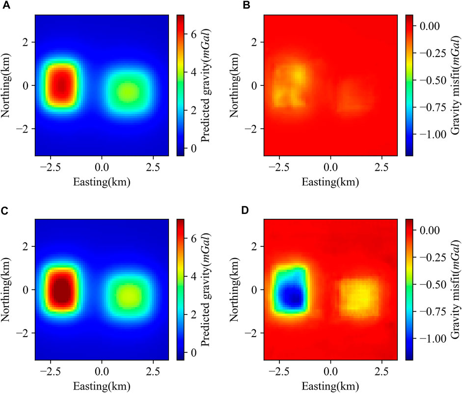
FIGURE 6. Predicted gravity anomaly and gravity misfit characteristics of horizontal distributed model (A) Gravity anomaly calculated by density contrast predicted by DGV-Net; (B) Gravity anomaly misfit produced by DGV-Net; (C) Gravity anomaly calculated by density contrast predicted by MGV-Net; (D) Gravity anomaly misfit produced by MGV-Net.

Table 3 summarizes the model relative error and the mean square error of recovered gravity. From Table 3, we found that the model relative errors don’t have a significant difference between DGV-Net and MGV-Net, this feature may illustrate that the two sorts of loss functions we used in this study have no distinct differences for GV-Net to predict simple density model.

2) Dipping dyke density model

TABLE 3

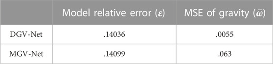
TABLE 3. The evaluating indicators of recovered horizontal distributed model.

The dipping dyke model is a classical 3D density model that can be used to evaluate the effectiveness of inversion methods (Zhu et al., 2020; Peng and Liu, 2021). Figure 7A illustrates a dipping dyke model and Figure 7B is the forward gravity. Figure 7C and Figure 7D are the inversion results predicted by DGV-Net and MGV-Net. Table 4 lists the relative error of the predicted models and the mean squared of gravity misfit. The prediction of DGV-Net recovered the shape of the true model mostly but exists a big bias in density value. The prediction of MGV-Net did not retrieve the true shape of the real model and the density value is also incorrect. But we found that the gravity misfit was not so bad as the density model, both models gave acceptable gravity misfit.

FIGURE 7

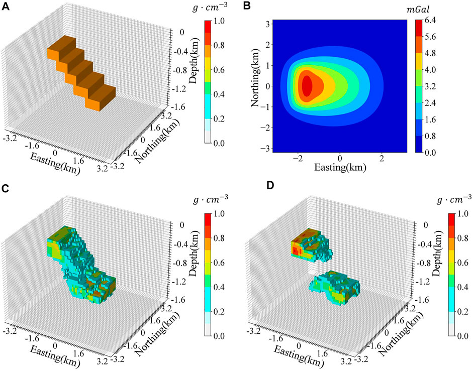
FIGURE 7. Dipping dyke density model (A) The shape of the dipping dyke density model; (B) Gravity anomalies that correspond to the true model; (C) The model recovered by DGV-Net; (D) The model recovered by MGV-Net.

TABLE 4

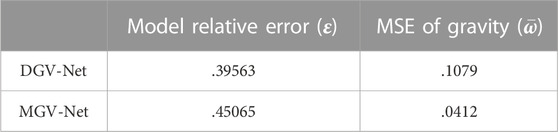
TABLE 4. The evaluating indicators of recovered dipping dike model.

Figure 8 shows the predicted gravity and gravity misfit of the dipping dyke model. From Figures 8A, C, the predicted gravity anomalies are generally consistent with input gravity anomalies, but the gravity anomalies misfit have obvious non-Gaussian characteristics (Figures 8B, D).

FIGURE 8

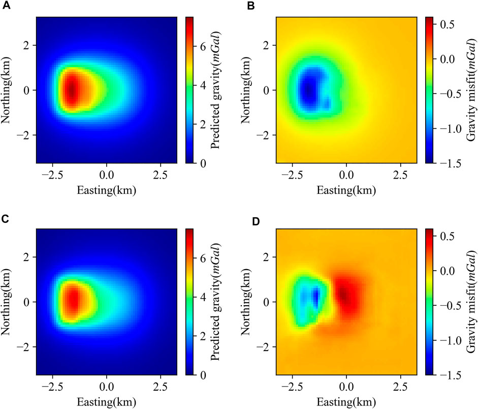
FIGURE 8. Predicted gravity anomaly and gravity misfit characteristics of dipping dyke model (A) Gravity anomaly calculated by density contrast predicted by DGV-Net; (B) Gravity anomaly misfit produced by DGV-Net; (C) Gravity anomaly calculated by density contrast predicted by MGV-Net; (D) Gravity anomaly misfit produced by MGV-Net.

In our training datasets, considering the generation strategy of our density model, models like dipping dyke are very rare. The GV-Net can recover this dipping dyke model proving that our method has the power to image the complicated density models even if they were not included in the training datasets.

3) Vertical distributed model

It is tough to revive vertical density information through gravity inversion. The conventional gravity inversion methods use the depth weighting function to control the density located in a suitable depth, but this process is depending on the researchers’ experience. To verify the performance of GV-Net to separate the density distribution in the vertical direction, we design an extreme vertical density model which means the different bodies have different depths but the same horizontal position (Figure 9A). It is difficult to intuitively retrieve any vertical characteristics from the forward gravity (Figure 9B).

FIGURE 9

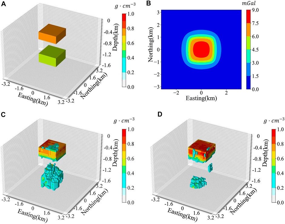
FIGURE 9. Vertical distributed model (A) The shape of the vertical distributed density model; (B) Gravity anomalies that correspond to the true model; (C) The model recovered by DGV-Net; (D) The model recovered by MGV-Net.

Table 5 summarized the model relative error and mean squared error of recovered gravity, from these two metrics, the DGV-Net has better performance in separating the density bodies in the vertical direction. Figure 9C and Figure 9D show the inversion results, the shallow body is well predicted by both DGV-Net and MGV-Net, but for the deeper body, the DGV-Net shows better results than MGV-Net.

TABLE 5

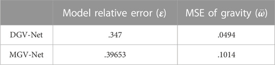
TABLE 5. The evaluating indicators of recovered vertical distribute density model.

The predicted gravity and gravity misfit of the vertical distributed model are shown in Figure 10. The gravity misfit produced by MGV-Net is obviously bigger than that obtained by DGV-Net.

FIGURE 10

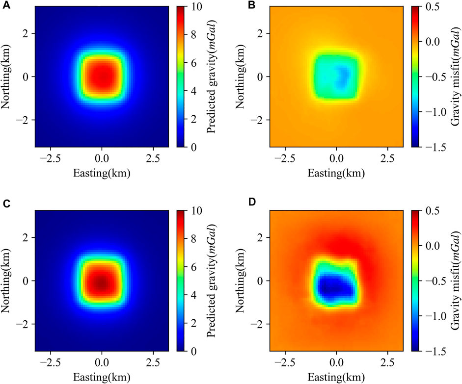
FIGURE 10. Predicted gravity anomaly and gravity residual characteristics of vertical distributed model (A) Gravity anomaly calculated by density contrast predicted by DGV-Net; (B) Gravity anomaly misfit produced by DGV-Net; (C) Gravity anomaly calculated by density contrast predicted by MGV-Net; (D) Gravity anomaly misfit produced by MGV-Net.

4.3 Noise effect

Actual gravity data is affected by various factors, such as the observation environment, instrument features, and human operations, which inevitably contain a certain degree of noise. In most cases, these noises are stochastic. We assumed that the noise is Gaussian noise with zero mean. We found that the DGV-Net mostly outperforms the MGV-Net in the model prediction accuracy in section 4.1. Therefore, in this part, we chose DGV-Net to test the robustness to the noise of our method.

We first use the well-trained DGV-Net model in section 4.1 to deal with the noise-contained gravity. The true density model is shown in Figure 11A, and the forward gravity contaminated by 0%, 1%, 2%, 5%, and 10% Gaussian noise are shown in Figures 11B–F respectively. The results predicted by DGV-Net are shown in Figures 12A, C, E, G, I, these results illustrated that the DGV-Net model can accurately predict the density structure while the noise is less than 2%, and this model can’t retrieve any useful information when the noise increases to 5%.

FIGURE 11

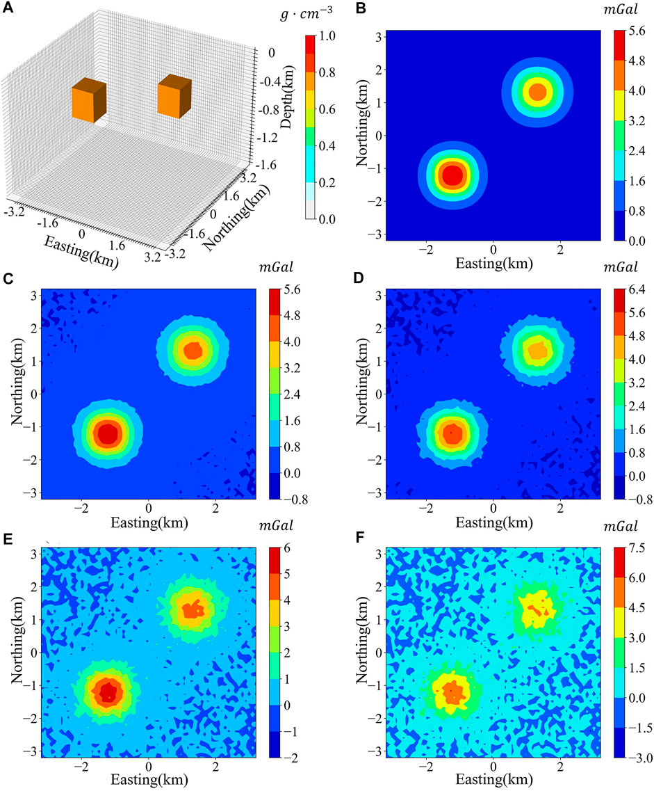
FIGURE 11. The density model and theoretical gravity with different noise levels. (A) The true model; (B) Gravity with noise-free; (C) Gravity with 1% Gaussian noise; (D) Gravity with 2% Gaussian noise; (E) Gravity with 5% Gaussian noise; (F) Gravity with 10% Gaussian noise.

FIGURE 12

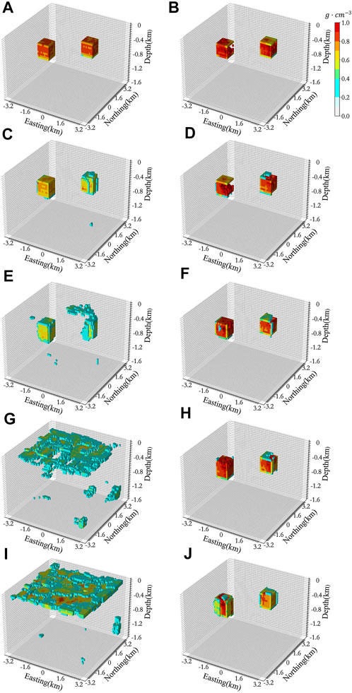
FIGURE 12. Results predicted by DGV-Net and NDGV-Net with various noise contained gravity data. Fig (A), (C), (E), (G) and (I) are the DGV-Net inversion results when the noise levels are 0%, 1%, 2%, 5% and 10%, respectively; Fig (B), (D), (F), (H) and (J) are the NDGV-Net inversion results when the noise levels are 0%, 1%, 2%, 5% and 10%, respectively.

We reproduced the training datasets that contain different noise strengths. 0%, .1%, .2%, .3%, .4%, .5%, 1%, 1.5%, 2%, 4% and 6% Gaussian noise was randomly added in the process of generating the training datasets, the occurrence probability of 0% noise level is 3/13, and the occurrence probability of other noise levels is 1/13. For the convenience of expression, we call the DGV-Net model trained by noise-contained datasets as NDGV-Net.

The results predicted by NDGV-Net are shown in Figures 12B, D, F, H, J, the density contrast can be effectively recovered even with the noise level up to 10%. However, the NDGV-Net model can restore the contour of density volume well, but it sacrifices the accuracy in density value prediction. Table 6 shows that the relative error of the result predicted by NDGV-Net for noise-free gravity is far greater than the result predicted by DGV-Net. These features illustrated that the robustness to noise of GV-Net is mainly controlled by the training datasets. It is important to balance the robustness and prediction accuracy through special noise setting of the training datasets for a specific inversion problem.

TABLE 6

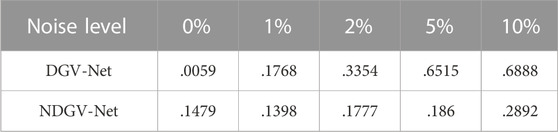
TABLE 6. The relative error(ε) of recovered models under different noise contained gravity for NDGV-Net and DGV-Net.

5 Case study

To verify the ability of the proposed method in this study to deal with real scenarios, we employed GV-Net to image the San Nicolas sulfide copper-zinc mine in Zacatecas, Mexico. The mining area has been studied in detail by different scholars using different inversion methods (Phillips et al., 2001; Lelièvre and Oldenburg, 2009; Zelin et al., 2019; Huizhen et al., 2021).

The residual Bouguer gravity anomaly is shown in Figure 13A, and the geological profiles in the location of AA′ and BB’ are shown in Figure 14, which are interpreted from logging data. On the basis of the size of the research region, orebody burial depth, and surrounding rock density characteristics, we regenerated the training datasets suitable for this mining area, and the new training datasets still divide the model into 32 × 64 × 64 three-dimensional cells, the size of a single cell is 25 m × 25 m × 25 m, and the density of the training datasets varies from .7 to 1.2 g/cm³ on the basis of prior information from the geological profiles. Considering that the actual data may be containing noise, the same noise addition strategy is adopted in the training datasets as in the NDGV-Net training datasets.

FIGURE 13

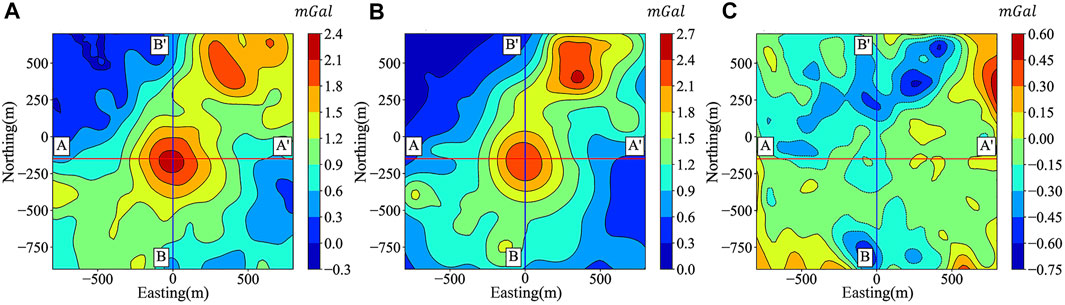
FIGURE 13. (A) Residual gravity anomaly map of the San Nicolas deposit (Huang et al., 2021); (B) Predicted gravity from invert density model; (C)Characteristics of gravity anomaly misfit.

FIGURE 14

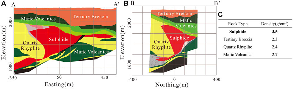
FIGURE 14. (A) Geologic cross-section along the AA′ line; (B) Geologic cross-section along the BB′ line; (C) Density of the major rock units.

We intercepted six two-dimensional profiles of the 3D density structure along the AA’, BB’ positions and its left and right 100 m, respectively. The corresponding cross-section results are shown in Figure 15, in order to clearly highlight the orebody position, only the voxels with a density greater than 0.6 g/cm³ is shown in Figure 15.

FIGURE 15

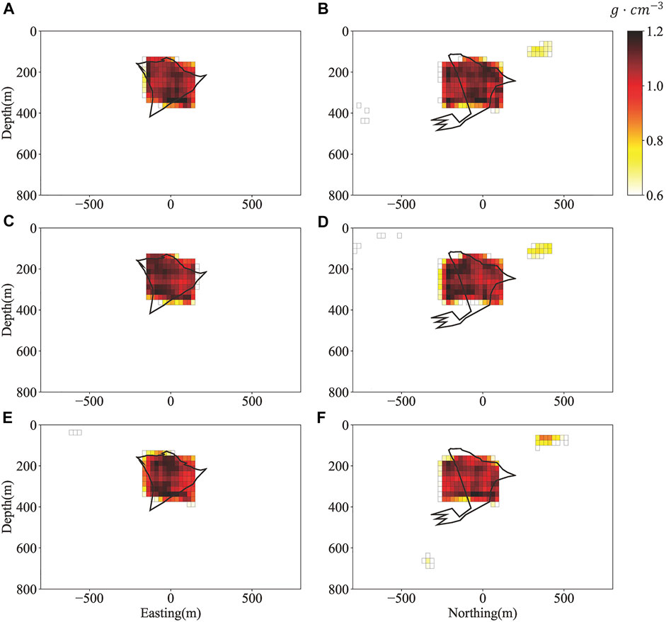
FIGURE 15. Inversion result at different cross-sections (The black lines indicate the true outline of the sulfide deposit) (A) Density Cross-section at AA′ line; (B) Density Cross-section at BB′ line; (C) Density Cross-section at 100 m south of AA′ line; (D) Density Cross-section at 100 m west of BB′ line; (E) Density Cross-section at 100 m north of AA′ line; (F) Density Cross-section at 100 m east of AA′ line.

Figures 13B, C are the predicted gravity anomalies and gravity misfit, respectively. We can see that the predicted gravity anomalies and true gravity anomalies have the same change trend, but there is a certain large and non-normal distribution of gravity misfit characteristics.

The predicted results in Figure 15 shows that our inversion method accurately restores the orebody position. The ore body size is basically the same as the real ore, but the ore body morphology is more like a regular prism, which should be related to the characteristics of the training datasets adopted in this article. Compared to the application of traditional inversion methods in this area (Phillips et al., 2001; Zelin et al., 2019; Huizhen et al., 2021), our method obtained a desirable result through the trained ML model based on targeted training datasets and no longer rely on the subjective experience of researchers.

6 Conclusions and discussions

This study purposes a CNN model named GV-Net, which implements inversion of the residual Bouguer gravity anomaly based on the ML technique. We first analyzed the effect of different loss functions on the GV-Net model and evaluated the prediction accuracy by three typical density contrast models. Then we tested the robustness to noise of our method by the noise or noise-free training datasets. Ultimately, the practicability of the method has been demonstrated by actual mining area data. The main conclusions of this research are as follows:

1) The selection of the loss function will influence the training speed, convergence characteristics, and model prediction accuracy. In this study, the Dice_Loss function has better performance in model prediction accuracy, and the MSE_Loss needs less time for the training process. Therefore, when we try to solve a practical problem, an appropriate loss function should be selected on the basis of weighing the prediction accuracy of the model against the training time cost of the model.

2) From the three synthetic tests, our GV-Net model has shown the ability to revive the shape of shallow density contrast, but it still lacks sufficient recovery for the abnormal density distribution of complex structures or abnormal bodies with obvious vertical distribution characteristics. There is no significant difference between DGV-Net and MGV-Net in predicting simple density models, but for sophisticated models, the DGV-Net has better performance in depicting the shape of density blocks. The mean squared error of gravity is acceptable for three synthetic models, but it seems independent of the relative error of the model. This feature may be caused by the absence of gravity constraint in the model training phase.

3) The robustness to noise of the GV-Net is closely related to the noise characteristics in the training datasets. While training datasets are designed by reasonable noise control, the anti-noise ability of the model is significantly improved.

4) In the GV-Net model, prior knowledge is directly included in the training dataset, rather than relying on the experience of researchers that is required by traditional inversion methods. When we predict a density anomaly body using the trained model, only the gravity anomaly is required as input, and we will obtain a reasonable result.

5) Using the GV-Net model to solve inversion problems, the training process is also time-consuming. But if a suitable AI model with good generalization ability can be achieved, the time needed to invert a density model is very small. The single prediction time of all models in this study is in milliseconds which demonstrated that our method can be used to fast imaging for specific inversion problems.

6) Using GV-Net for inversion of actual mining area data, the results are consistent with previous studies, which demonstrates the practicability of this method.

Although the method proposed in this study can better realize the fast inversion of residual Bouguer gravity anomaly, there are still some problems that need to be further solved, such as how to construct a training dataset that can represent real geologically density distribution better. In addition, in the model prediction process, the gravity data is used as the input to directly invert the three-dimensional density model, and the gravity misfit shown certain non-stochastic characteristics.

Data availability statement

The original contributions presented in the study are included in the article/supplementary material, further inquiries can be directed to the corresponding author.

Author contributions

YL, SC, BZ, and HL designed the research. BZ and YL designed the model and wrote the program code. SC contributed to building the synthetic model and interpretation the inversion result. YL and HL drew figures and tables and wrote the first draft of the manuscript. All authors revised the manuscript and approved the version to be published.

Funding

This work is jointly supported by the National Key R&D Program of China (2017YFC1500503), and the National Natural Science Foundation of China (Grant U1939205, 42004069, 42104090).

Conflict of interest

The authors declare that the research was conducted in the absence of any commercial or financial relationships that could be construed as a potential conflict of interest.

Publisher’s note

All claims expressed in this article are solely those of the authors and do not necessarily represent those of their affiliated organizations, or those of the publisher, the editors and the reviewers. Any product that may be evaluated in this article, or claim that may be made by its manufacturer, is not guaranteed or endorsed by the publisher.

References

Andersson, T. R., Hosking, J. S., Perez-Ortiz, M., Paige, B., Elliott, A., Russell, C., et al. (2021). Seasonal Arctic sea ice forecasting with probabilistic deep learning. Nat. Commun. 12 (1), 5124. doi:10.1038/s41467-021-25257-4

PubMed Abstract | CrossRef Full Text | Google Scholar

Bergen, K. J., Johnson, P. A., de Hoop, M. V., and Beroza, G. C. (2019). Machine learning for data-driven discovery in solid Earth geoscience. Science 363 (6433), eaau0323. doi:10.1126/science.aau0323

PubMed Abstract | CrossRef Full Text | Google Scholar

Bosch, M., Meza, R., Jiménez, R., and Hönig, A. (2006). Joint gravity and magnetic inversion in 3D using Monte Carlo methods. Geophysics 71 (4), G153–G156. doi:10.1190/1.2209952

CrossRef Full Text | Google Scholar

Chen, T., and Zhang, G. (2022). Mineral exploration potential estimation using 3D inversion: A comparison of three different norms. Remote Sens. 14 (11), 2537. doi:10.3390/rs14112537

CrossRef Full Text | Google Scholar

Davis, K., and Li, Y. (2011). Fast solution of geophysical inversion using adaptive mesh, space-filling curves and wavelet compression. Geophys. J. Int. 185 (1), 157–166. doi:10.1111/j.1365-246X.2011.04929.x

CrossRef Full Text | Google Scholar

Foks, N. L., Krahenbuhl, R., and Li, Y. (2014). Adaptive sampling of potential-field data: A direct approach to compressive inversion. Geophysics 79 (1), IM1–IM9. doi:10.1190/geo2013-0087.1

CrossRef Full Text | Google Scholar

Fu, G., Gao, S., Freymueller, J. T., Zhang, G., Zhu, Y., and Yang, G. (2014). Bouguer gravity anomaly and isostasy at Western Sichuan Basin revealed by new gravity surveys. J. Geophys. Res. Solid Earth 119 (4), 3925–3938. doi:10.1002/2014jb011033

CrossRef Full Text | Google Scholar

He, S., Cai, H., Liu, S., Xie, J., and Hu, X. (2021). Recovering 3D basement relief using gravity data through convolutional neural networks. J. Geophys. Res. Solid Earth 126 (10). doi:10.1029/2021jb022611

CrossRef Full Text | Google Scholar

Honglei, L., Shi, C., Jiancang, Z., Bei, Z., and Lei, S. (2021). Gravity inversion method base on Bayesian-assimilation and its application in constructing crust density model of the Longmenshan region. Chin. J. Geophys. Chin. 64 (4), 1263–1252. doi:10.6038/cjg2021O0130

CrossRef Full Text | Google Scholar

Huang, R., Liu, S., Qi, R., and Zhang, Y. (2021). Deep learning 3D sparse inversion of gravity data. J. Geophys. Res. Solid Earth 126. doi:10.1029/2021jb022476

CrossRef Full Text | Google Scholar

Huizhen, Y., Jinduo, W., and Qianjun, W. (2021). Gravity inversion based on sparse representation of density model. Chin. J. Geophys. Chin. 64 (3), 1061–1073. doi:10.6038/cjg2021O0113

CrossRef Full Text | Google Scholar

Johannes, W. J., and Smilde, P. L. (2009). Gravity interpretation: Fundamentals and application of gravity inversion and geological interpretation[M]. Springer.

Google Scholar

Kong, Q., Trugman, D. T., Ross, Z. E., Bianco, M. J., Meade, B. J., and Gerstoft, P. (2018). Machine learning in seismology: Turning data into insights. Seismol. Res. Lett. 90 (1), 3–14. doi:10.1785/0220180259

CrossRef Full Text | Google Scholar

Lelièvre, P. G., and Oldenburg, D. W. (2009). A comprehensive study of including structural orientation information in geophysical inversions. Geophys. J. Int. 178 (2), 623–637. doi:10.1111/j.1365-246X.2009.04188.x

CrossRef Full Text | Google Scholar

Lelièvre, P. G., Farquharson, C. G., and Hurich, C. A. (2012). Joint inversion of seismic traveltimes and gravity data on unstructured grids with application to mineral exploration. Geophysics 77 (1), K1–K15. doi:10.1190/geo2011-0154.1

CrossRef Full Text | Google Scholar

Li, Y. G., and Oldenburg, D. W. (1998). 3-D inversion of gravity data. Geophysics 63 (1), 109–119. doi:10.1190/1.1444302

CrossRef Full Text | Google Scholar

Li, Y., and Oldenburg, D. W. (1996). 3-D inversion of magnetic data. Geophysics 61 (2), 394–408. doi:10.1190/1.1443968

CrossRef Full Text | Google Scholar

Liu, S., Jin, S., Xuan, S., and Liu, X. (2022). 3-D data-space joint inversion of gravity and magnetic data using a correlation-analysis constraint. Ann. Geophys. 65. doi:10.4401/ag-8750

CrossRef Full Text | Google Scholar

Milletari, F., Navab, N., and Ahmadi, S-A. (2016). “V-Net: Fully convolutional neural networks for volumetric medical image segmentation,” in 2016 Fourth International Conference on 3D Vision (3DV), 565–571.

CrossRef Full Text | Google Scholar

Ming, Z., Shi, C., and Yuen, D. (2019b). Waveform classification and seismic recognition by convolution neural network. Chin. J. Geophys. Chin. 62 (1), 374–382. doi:10.6038/cjg2019M0151

CrossRef Full Text | Google Scholar

Ming, Z., Shi, C., LiHua, F., and Yuen, D. A. (2019a). Earthquake phase arrival auto-picking based on U-shaped convolutional neural network. Chin. J. Geophys. Chin. 62 (8), 3034–3042. doi:10.6038/cjg2019M0495

CrossRef Full Text | Google Scholar

Mitra, R., Naruse, H., and Abe, T. (2020). Estimation of tsunami characteristics from deposits: Inverse modeling using a deep-learning neural network. J. Geophys. Res. Earth Surf. 125 (9). doi:10.1029/2020jf005583

CrossRef Full Text | Google Scholar

Nagy, D., Papp, G., and Benedek, J. (2000). The gravitational potential and its derivatives for the prism. J. Geodesy 74 (7-8), 552–560. doi:10.1007/s001900000116

CrossRef Full Text | Google Scholar

Peng, G., and Liu, Z. (2021). 3D inversion of gravity data using reformulated L -norm model regularization. J. Appl. Geophys. 191, 104378. doi:10.1016/j.jappgeo.2021.104378

CrossRef Full Text | Google Scholar

Phillips, N., Oldenburg, D., Chen, J., Li, Y., and Routh, P. (2001). Cost effectiveness of geophysical inversions in mineral exploration: Applications at San Nicolas. Lead. Edge 20 (12), 1351–1360. doi:10.1190/1.1487264

CrossRef Full Text | Google Scholar

Ronneberger, O., Fischer, P., and Brox, T. (2015). U-Net: Convolutional networks for biomedical image segmentation. Lect. Notes Comput. Sci. 9531, 234–241. doi:10.1007/978-3-319-24574-4_28

CrossRef Full Text | Google Scholar

Rosid, M. S., Riska, I. A., and Jaman, A. P. (2020). 3D inversion modelling of gravity data to identify gold mineralization zones in region “X”, Pongkor. IOP Conf. Ser. Earth Environ. Sci. 481 (1), 012049. doi:10.1088/1755-1315/481/1/012049

CrossRef Full Text | Google Scholar

Shen, C. (2018). A transdisciplinary review of deep learning research and its relevance for water resources scientists. Water Resour. Res. 54 (11), 8558–8593. doi:10.1029/2018wr022643

CrossRef Full Text | Google Scholar

Turing, A. M. (1950). I.—computing machinery and intelligence. Mind LIX (236), 433–460. doi:10.1093/mind/LIX.236.433

CrossRef Full Text | Google Scholar

Valentine, A., and Kalnins, L. (2016). An introduction to learning algorithms and potential applications in geomorphometry and Earth surface dynamics. Earth Surf. Dyn. 4 (2), 445–460. doi:10.5194/esurf-4-445-2016

CrossRef Full Text | Google Scholar

Wang, Q., Ma, Y., Zhao, K., and Tian, Y. (2020). A comprehensive survey of loss functions in machine learning. Ann. Data Sci. 9 (2), 187–212. doi:10.1007/s40745-020-00253-5

CrossRef Full Text | Google Scholar

Wang, X., Fang, J., and Hsu, H. (2014). Three-dimensional density structure of the lithosphere beneath the North China Craton and the mechanisms of its destruction. Tectonophysics 610, 150–158. doi:10.1016/j.tecto.2013.11.002

CrossRef Full Text | Google Scholar

Zelin, L., Changli, Y., and Yuanman, Z. (2019). 3D inversion of gravity data using Lp-norm sparse optimization. Chin. J. Geophys. Chin. 62 (10). doi:10.6038/cjg2019M0430

CrossRef Full Text | Google Scholar

Zhu, W., Peng, J., Luo, S., Meng, X., Liu, J., and Zhu, C. (2020). Gravity sparse inversion using the interior-point method and a general model weighting function. Studia Geophys. Geod. 64 (4), 419–435. doi:10.1007/s11200-020-0831-5

CrossRef Full Text | Google Scholar