Lava fountain jet noise during the 2018 eruption of fissure 8 of Kīlauea volcano

Real-time monitoring is crucial to assess hazards and mitigate risks of sustained volcanic eruptions that last hours to months or more. Sustained eruptions have been shown to produce a low frequency (infrasonic) form of jet noise. We analyze the lava fountaining at fissure 8 during the 2018 Lower East Rift Zone eruption of Kīlauea volcano, Hawaii, and connect changes in fountain properties with recorded infrasound signals from an array about 500 m from the fountain using jet noise scaling laws and visual imagery. Video footage from the eruption reveals a change in lava fountain dynamics from a tall, distinct fountain at the beginning of June to a low fountain with a turbulent, out-pouring lava pond surrounded by a tephra cone by mid-June. During mid-June, the sound pressure level reaches a maximum, and peak frequency drops. We develop a model that uses jet noise scaling relationships to estimate changes in volcanic jet diameter and jet velocity from infrasound sound pressure levels and peak frequencies. The results of this model indicate a decrease in velocity in mid-June which coincides with the decrease in fountain height. Furthermore, the model results suggest an increase in jet diameter, which can be explained by the larger width of the fountain that resembles a turbulent lava pond compared to the distinct fountain at the beginning of June. The agreement between the infrasound-derived and visually observed changes in fountain dynamics suggests that jet noise scaling relationships can be used to monitor lava fountain dynamics using infrasound recordings.

1 Introduction

Sustained volcanic eruptions can pose a variety of hazards to life and infrastructure, and recognizing and understanding changes in eruption dynamics is critical to mitigate the risk (Houghton et al., 2021; Meredith et al., 2022). Ideally, the characterization of eruptions should be done remotely and independent of weather and light conditions to minimize exposure of scientists in the field and assure constant surveillance. The use of infrasound has been proven effective in characterizing eruption dynamics (e.g., Fee and Matoza, 2013; Ulivieri et al., 2013; Ripepe et al., 2018; Watson et al., 2022). Acoustic waves are characterized as infrasound when their frequencies are below 20 Hz. Atmospheric absorption at these low frequencies is minor and waves can travel tens to thousands of kilometers around the Earth (Sutherland and Bass, 2004; Dabrowa et al., 2011; Matoza et al., 2022). Detailed analysis of short duration, impulsive eruptions has shown that the representation of the source as monopole and dipole can yield good estimations of eruptive mass, volume and directivity (e.g., Johnson and Miller, 2014; Kim et al., 2015; Yamada et al., 2018; Iezzi et al., 2019). However, sustained eruptions without distinct explosions and continuous discharge of gas and solids are often more difficult to analyze (Fee et al., 2017; Sciotto et al., 2019). Volcanic jets have been shown to produce sound similar to anthropogenic jets, such as jet engines (Matoza et al., 2009, 2013; Gestrich et al., 2021), and one way to characterize eruption infrasound is by utilizing knowledge from laboratory jet noise studies. In particular the spectral shape of volcanic eruption noise is remarkably similar to jet noise (Matoza et al., 2009, 2013; Gestrich et al., 2021). Lava fountains are a specific expression of sustained eruptions, and due to their diversity in dynamics, multiple source generation mechanisms have been proposed such as oscillatory motion of lava during churn flow Ulivieri et al. (2013), bubble bursting, and also jet noise (Lamb et al., 2022). By understanding the source of the acoustics recorded during lava fountain activity, we may connect changes of acoustic parameters to changes in the lava fountain dynamics. Detecting changes in lava fountain dynamics from a remote location in real time would enable fast and efficient reaction to hazards such as lava flows from changing activity (Lyons et al., 2021).

Here, we explore the relationship between the recorded infrasound signals and documented dynamics of the eruption of fissure 8, of Kīlauea in 2018. We use Uncrewed Aircraft System (UAS) video footage as well as published lava and SO₂ discharge analysis by Dietterich et al. (2021), Kern et al. (2020), and Lerner et al. (2021) to characterize the change in eruption dynamics between June 4 and July 14. Infrasound recordings from a four element array that was installed close to the fissure are used to obtain acoustic parameters such as frequency content and amplitude. Audible sound during the eruption was often described as if jet engines were taking off (Sylvester, 2018), which is consistent with the similarity between the recorded acoustic spectrum during the eruption and semi-empirical jet noise spectra as shown by Gestrich et al. (2021). The semi-empirical jet noise similarity spectra were developed by Tam et al. (1996) by analyzing a large dataset of laboratory scale jet noise recordings. Details are described in Section 2.3. Here, we use jet noise scaling relationships to invert the calculated infrasound parameters to jet velocity and diameter. As gas and lava dynamics are closely connected in lava fountains (Parfitt et al., 1995; Wilson et al., 1995), the detection of changes in jet velocity and diameter can be used as an indicator for similar changes in the lava fountain.

We divide our analysis into three time periods of 2018: June 4–16, June 16–July 14, and July 14–31, relating to changes in the eruption dynamics discussed in Section 5.1 and acoustic properties discussed in Section 5.2. Specifically, the end of the first time window on June 16 is determined by the decrease in peak frequency and peak in sound pressure level of the infrasound recordings. The third time window marks the primary time window of pulses described in (Lyons et al., 2021). These three time windows are colored blue, red, and yellow in our Figures 1, 5, 7, 8 with labeled time stamps at the top of each figure. The eruption diminished significantly after August 5, which we shade in green with striped pattern.

FIGURE 1

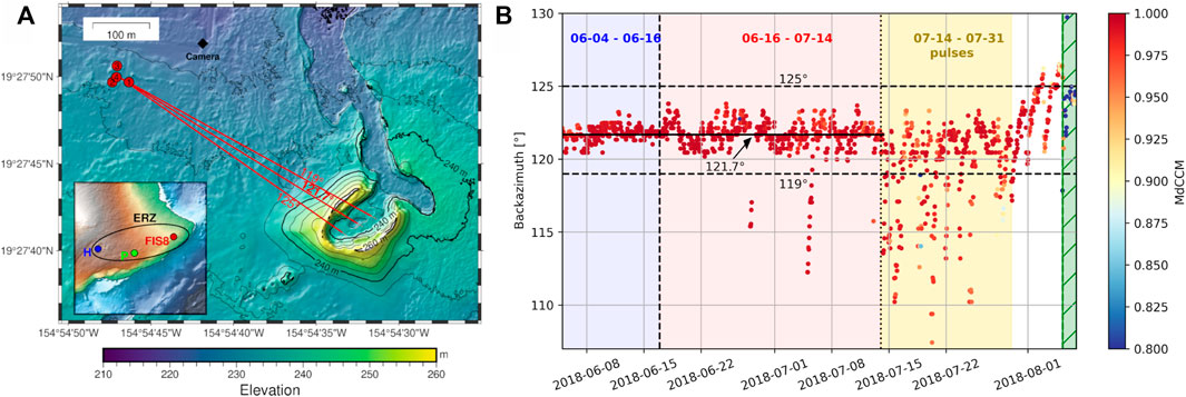
FIGURE 1. Location of the infrasound array and vent and array processing results. (A) Shows the location of the infrasound sensors (red circles) in relation to the erupting fissure. The red dashed and dotted lines refer to the backazimuth calculation shown in (B) The black diamond shows the location of the time-lapse (TL) camera used for estimating the cone growth in Figure 3. The insert map shows the location of mentioned places on the Island of Hawai‘i, including Halema‘uma‘u crater (H), East Rift Zone (ERZ), Pu‘u‘ō‘ō vent (P) and the location of fissure 8 and the infrasound array (FIS8). (B) Shows the backazimuth results for array FIS8. The colors correspond to the median cross correlation maxima (MdCCM) value. The solid black line is the median backazimuth for the time before the majority of the pulses start (before July 14). The dashed lines indicate the approximate extend of backazimuth fluctuations before the pulses. These three backazimuths are shown on the map in (A). The background colors and vertical dashed and dotted lines in (B) differentiate the time windows labeled in the according colors at the top of the figure.

2 Background

2.1 Lava fountain dynamics

Lava fountains are influenced by many different parameters, like viscosity, volatile content, and magma recharge, that affect the velocity of magma and gas before fragmentation, during fragmentation, and when entering the surrounding atmosphere (Parfitt et al., 1995). In low viscosity, basaltic magma typical for eruptions of Kīlauea, exsolved volatiles form bubbles that are buoyant with respect to the surrounding melt and can move vertically through it (Gonnermann and Manga, 2007). If the magma rise speed is relatively slow, the bubbles can coalesce and form large bubbles that burst at the surface of the magma column in distinct explosions, which are classified as Strombolian-style explosion (Parfitt, 2004; Taddeucci et al., 2015). On the other hand, Hawaiian-style lava fountains can occur when the magma rise speed is relatively fast so that the exsolved bubbles cannot coalesce (Wilson and Head, 1981). The transition between Hawaiian- and Strombolian-style eruptions is marked by lower fountain heights and occasional distinct explosions. When magma rises in the upper crust, the decrease in pressure leads to further gas expansion, acceleration and disruption (Parfitt and Wilson, 1995). Close to the surface, re-entrapment of lava can significantly reduce lava fountain height (Wilson et al., 1995). This happens when lava clasts fall back into the vent and get mixed with the freshly erupting magma. The effect gets noticeable when pyroclasts falling close to the vent form a pond surrounding the lava fountain, which can, in extreme cases, suppress a fountain completely (Parfitt et al., 1995). As the ascending porous magma fragments and interacts with the lava pond at the vent, pyroclast ejection velocity is reduced. After entering the atmosphere, without any additional forces, the pyroclasts can be considered to generally obey a simplistic ballistic equation for fountain height H = u²/(2g), with g being the gravitational acceleration and u the initial velocity of the observed object (Wilson and Head, 1981). These pyroclast can be accelerated by the drag force applied by the gas expansion (Parfitt et al., 1995). Therefore clast and gas velocity above the vent are mutually related (Wilson et al., 1995).

Quantifying lava fountain properties is challenging, particularly in real-time. Video, radar, gas sampling, and other techniques provide insight into fountain dynamics but are hampered by measurement uncertainties and deployment and safety challenges (Evans and Staudacher, 2001; Witt and Walter, 2017; Mereu et al., 2020). Infrasound provides one technique for examining lava fountains, as they can be prolific producers of low-frequency and audible acoustic waves (e.g., Fee et al., 2011; Sciotto et al., 2019; Lamb et al., 2022). Here, we will use the analogy between laboratory jets and the gas release during lava fountain events to determine the gas velocity and vent diameter. This analysis and interpretation has the potential to be used on real-time data in the future, which are available for many volcanoes. The use of real-time infrasound signals, as opposed to visual measurements, has the advantage to work remotely without interruptions due to visibility. We note that the influence of wind and topographic effects on sound propagation should also be considered, and here we address those in the Supplementary Section S1.1 and Sections 4.2, 5.3.

2.2 The 2018 lower East Rift Zone eruption of Kīlauea volcano

Kīlauea volcano on the Island of Hawai‘i is the youngest and most active Hawaiian volcano with recent eruptions at the summit in the Halema‘uma‘u crater and along the East Rift Zone (ERZ) at Pu‘u‘ō‘ō vent (labeled in Figure 1) and the lower East Rift Zone (LERZ), which is the most eastern part of the ERZ (Neal et al., 2019). After a period of sustained ground inflation, the activity in 2018 accelerated, starting with the collapse of the Pu‘u‘ō‘ō vent on 30 April 2018, accompanied by increased seismicity and the drainage of the Halema‘uma‘u lava lake in the following days (Patrick et al., 2018; Anderson et al., 2019; Neal et al., 2019). On May 3, an eruption in the LERZ began with the opening of the first active fissure (fissure 1) Neal et al. (2019). Eruptive activity was coincident with significant deformation of the volcano, including a M 6.9 earthquake on May 4 and widespread collapse of the summit caldera for the duration of the eruption. After opening multiple fissures in various locations along the LERZ, the activity focused on fissure 8 (F8), building a cone later named Ahu‘ailā‘au, at the end of May. The location and post-eruptive DEM is shown in Figure 1. The eruption rate diminished significantly on August 5, with weak residual effusion until September 5, when the eruption ended.

The activity at fissure 8 primarily consisted of lava fountaining up to 80 m in height (Neal et al., 2019), feeding a spillway that broadened into a large lava flow north and east of the fissure (Dietterich et al., 2021; Lyons et al., 2021). The erupted basalts had similar compositions to eruptions before 2018 that were sourced from the Kīlauea summit region (Gansecki et al., 2019; Pietruszka et al., 2021). The effusion rate grew slowly, peaking in mid-June at approximately 350 m³s⁻¹ and continuing with relatively high effusion rates of ca. 250 m³s⁻¹ until the end of the eruption in the beginning of August (Dietterich et al., 2021). Beginning as early as mid-June, surges in effusion rate occurred, which are described by Patrick et al. (2019) as long-term fluctuations following collapse events at the volcano’s summit. They were characterized by an increase in bulk effusion rate for approximately 4–6 h followed by a slower decrease. A correlation between bulk-effusion rate and infrasound points to a similar gas content and outgassing mechanism throughout (Patrick et al., 2019; Dietterich et al., 2021). Pulses were another short-duration fluctuation in bulk lava effusion rate, presumed to be due to variations in outgassing efficiency (Patrick et al., 2019). They led to a change of the center of the infrasound source between vent location and spillway and occurred in the period of mid July through the beginning of August (Lyons et al., 2021). Due to the large and rapid changes in infrasound location and outgassing mechanisms during this period of pulsing, we will not focus on the time between July 14–31 in our analysis. Gas measurements and estimations show a similar general trend as the bulk effusion rate with an increase in SO₂ throughout the beginning of June with a peak in mid-June (Kern et al., 2020; Vernier et al., 2020; Lerner et al., 2021).

2.3 Jet noise

Jetting is the introduction of a fast fluid into a comparably still medium through a small opening. Volcanic eruptions are known to rapidly discharge gas and solids into the atmosphere. This initial momentum-driven phase has been called jetting in the literature (e.g., Kieffer, 1984; Roche and Carazzo, 2019), pointing to the similar fluid dynamics that are observed for anthropogenic and laboratory jets. This analogy is strengthened by the nature of self similarity within jets, which means that similar features are observed at a wide range of jet dimensions, ranging from small laboratory jets with nozzle openings on the order of millimeters to centimeters to volcanic jets that can be up to hundreds of meters (Matoza et al., 2009; Fee et al., 2010b).

The sound produced by jets has been studied extensively by acousticians and engineers with goals ranging from fundamental research to noise reduction and optimized performance of industrial jets (e.g., Seiner and Gilinsky, 1995). Tam et al. (1996) identified two scales of turbulence that produce jet noise with distinct spectral shapes. Large scale turbulence (LST) noise is produced by coherent instability waves that emanate close to the nozzle region. This noise is dominant in a cone-shaped area around the center axis of the jet. In the jet noise literature, observation angles are typically measured with respect to the downward pointing jet axis. This means that 180° corresponds to a position exactly above the jet nozzle. Large scale turbulence is typically observed at angles above 120° (Tam et al., 2008). Fine scale turbulence (FST) noise, on the other hand, is produced by small incoherent turbulent motion and dominates outside of the LST cone. The spectral shapes described by (Tam et al., 1996) have been used to identify low frequency jet noise during volcanic eruptions (e.g., Matoza et al., 2009, 2013; Taddeucci et al., 2014; Gestrich et al., 2021; Lamb et al., 2022). Jet flow can exhibit a variety of other features that produce acoustic signals such as the vortex ring at the beginning of the jet formation (Fernández and Sesterhenn, 2017; Taddeucci et al., 2021) and crackle during supersonic jet flow (Fee et al., 2013). However, due to the sustained nature of the lava fountain activity, we do not expect any vortex ring formation and we will not investigate crackle noise as there is are no audible reports of such and a lack of skewness (see Supplementary Figure S1 and Section 5.2). Other jet specific noises typical for laboratory jets such as broadband shock noise and screech tones have typically been neglected for volcanic infrasound (Matoza et al., 2009, 2013). Laboratory jets used for studies such as Tam et al. (1996) are typically gas-only jets through comparably small nozzles and with a maximum jet temperature T_j of 3.2 times the ambient temperature T_a (Viswanathan, 2004). In contrast, volcanic jets typically comprise a mixture of gas, solid particles and molten rock in various ratios and temperatures of up to 1,150°C (Gansecki et al., 2019), which is 57 times an ambient temperature of T_a =20°C or 2.5–5.75 times an ambient temperature close to a lava fountain of T_s =200–400°C (Namiki et al., 2021). The effect of the solids and liquids and the increased temperature ratios are not well understood yet and will need future investigation.

2.3.1 Scaling relationships

Matoza et al. (2013) suggested that some scaling relationships developed for anthropogenic jets may be carefully applied to volcanic jets, such as the relationship between acoustic amplitude and jet velocity and diameter. Note that although similarities between volcanic and anthropogenic jets and their associated jet noise exist, notable differences, mentioned above, and inherent uncertainties require careful evaluation of their applicability.

Acoustic amplitude is usually expressed as sound pressure level (SPL), acoustic intensity, I, or acoustic power, Π, which we define following Garcés et al. (2013) and shown in Eq. 1; Supplementary Eqs S1–S5. Definitions and usage of these quantities vary slightly in the literature, especially with regards to differentiating SPL and intensity. In the following we restrict our analysis to relatively robust scaling relationships that have been developed for laboratory-scale jet noise.

The sound pressure level (SPL) is a parameter that represents the acoustic amplitude. Following Garcés et al. (2013) we define the SPL as:

$SPL=10{\log }_{10}\left(\frac{p_{\mathit{rms}}^2}{p_{\mathit{ref}}^2}\right)(1)$

$\mathrm{w}\mathrm{i}\mathrm{t}\mathrm{h}:p_{\mathit{rms}}^2=⟨p^2⟩=\frac{1}{T_s}{\int }_0^{T_s}{p}^2\left(t\right)dt,(2)$

With p being the recorded pressure, T_s being a time window of choice and p_ref = 2 × 10⁵ Pa the reference pressure.

Previous studies such as Viswanathan (2004), Viswanathan (2006), Viswanathan (2009), and Tam (2019) showed direct proportionalities between the acoustic intensity, power, and the jet velocity, v_j, and diameter, D_j, for anthropogenic jets, with the applicability to volcanic jets summarized by Matoza et al. (2013). The jet velocity dependence has exponents n_I (θ, T_j/T_a) and n_Π(T_j/T_a) for the intensity and power and are discussed below in more detail. Viswanathan (2006) and Matoza et al. (2013) expressed the proportionality between acoustic intensity, I, and power, Π, and jet velocity as.

$I\propto {\left(\frac{v_j}{c}\right)}^{n_I}(3)$

$\mathrm{\Pi }\propto {\left(\frac{v_j}{c}\right)}^{n_{\mathrm{\Pi }}},(4)$

With c being the speed of sound.

Furthermore, Matoza et al. (2013), following Tam (2005), reported a direct relationship between acoustic intensity (or sound pressure level) and squared jet diameter D_j.

$I\propto \frac{D_j^2}{r^2}{\left(\frac{v_j}{c}\right)}^{n_I}\underset{\begin{array}{c}\text{atmospheric}\\ \text{conditions}\end{array}}{\underbrace{\left({\rho }_{0}c{p}_0^2\right)}},(5)$

with ρ₀ and p₀ being the ambient density and pressure, both of which we assume to be constant. The jet diameter is normalized by the squared source-distance r to account for geometrical spreading of the acoustic wave.

Since the SPL is directly related to the acoustic intensity (see Supplementary Eq. S4), we can express the proportionality in Eq. 3 as.

$10^{SPL/10}\propto \frac{D_j^2}{r^2}{\left(\frac{v_j}{c}\right)}^{n_I}(6)$

$\iff SPL\propto 10{\log }_{10}\left(\frac{D_j^2}{r^2}\right)+10n_I{\log }_{10}\left(\frac{v_j}{c}\right).(7)$

We note that our infrasound data are recorded in the far-field of the source with the distance being approximately r=500 m. The far-field condition is met for $r\gg \frac{\lambda }{2\pi }\approx 54$ m at a frequency of 1 Hz and speed of sound of 335 m/s.

Importantly, we note the jet velocity exponents n_I for the acoustic intensity and n_Π for the acoustic power are different due to the directionality (directivity) of jet noise (Matoza et al., 2013). The velocity exponent for the acoustic power n_Π does not depend on the observation angle because the power is calculated by integrating over all angles. It has a slight temperature ratio dependence and varies between approximately n_Π = 7.98 to 8.74 for temperature ratios T_j/T_a = 3.2 to 1 (Viswanathan, 2004). Overall there is a slight decrease of the exponent value with rising temperature ratio but the exponent generally stays close to 8. The velocity exponent for the acoustic intensity n_I varies strongly with temperature ratio and observation angle. In Figure 16 in Viswanathan (2006) they show that at 90° relative to the jet axis (i.e., horizontal to nozzle) the exponent varies between approximately 5.8–8.1 for temperature ratios T_j/T_a = 3.2 to 1. The closer the angle gets to the jet axis, the more similar are values for n_I for different temperature ratios. The exponents generally increase the closer the angle to the jet axis and get up to approximately 10. Note that observed velocity exponents for jet noise differ from the simplified cases of monopole, dipole, or quadrupole radiation (Woulff and McGetchin, 1976). These cases are not necessarily applicable in the case of sustained jetting as explained in Matoza et al. (2013).

Viswanathan (2009) showed that the jet noise peak Strouhal number stays the same for different temperatures and jet velocities for an observation angle of approximately 90° from the jet axis. The assumption of a constant Strouhal number has been used in numerous volcano studies (Matoza et al., 2010; Fee et al., 2013; McKee et al., 2017; Haney et al., 2018). The non-dimensional peak Strouhal number is most commonly expressed as

$S{t}_p=\frac{f_p{D}_j}{v_j},(8)$

with f_p being the peak frequency (Mathews et al., 2021). Since the Strouhal number is dependent on the velocity and jet diameter, an increase in jet velocity or decrease in jet diameter results in an increase in peak frequency to accommodate the constant Strouhal number.

3 Data

3.1 Remote sensing data

Uncrewed Aircraft Systems (UAS) videos of the active fissure were taken most days throughout the eruption and published by DeSmither et al. (2021). Each video is only a few minutes long but provides an overall view of the activity during that day. Example videos from June 2, 10, 16, and 24 are provided in the Supplementary Video S1–S4. The videos are mostly oblique flybys, meaning that the angle, distance, and time varies during and between videos. We use these videos for qualitative description of the eruption dynamics and how it evolved through time. Selected single frames showing representative activity for certain days in June are shown in Figure 2 and described in Section 5.1. Ground-based time-lapse imagery was acquired and analyzed to derive outlines of the change of the Ahu‘ailā‘au cone profile shown in Figure 3. The location of the time-lapse camera is shown in Figure 1A.The post-eruptive topography is documented via an airborne lidar survey in July 2019 (Mosbrucker et al., 2020) and the DEM with 1 m resolution is shown in Figure 1A.

FIGURE 2

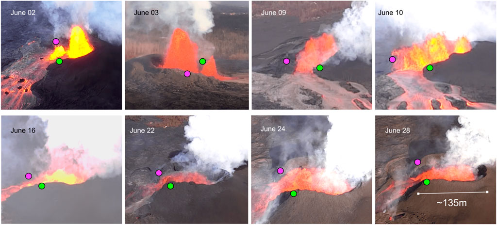
FIGURE 2. Single frames of UAS videos of the labeled days. These frames show representative activity observed in the respective videos. Note that these are taken from different view angles, distances and local times. The green and pink circles are reference points on each side of the spillway for easier orientation. A representative scale for the length of the fissure is shown on the photo of June 28.

FIGURE 3

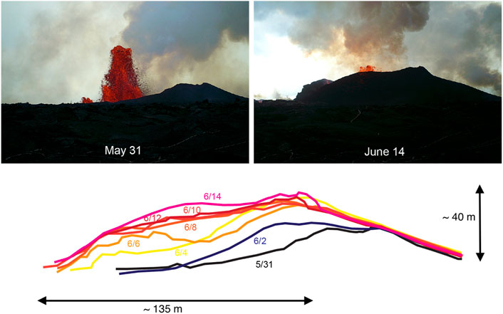
FIGURE 3. Sketch of cone profiles throughout the first half of June, derived from video frames. The top two figures show the camera view on May 31 and June 14 as an example of the cone growth. The location of the camera is shown in Figure 1A. The bottom sketch shows the outline of the cone as seen from the orientation of the camera for the days in between. Each line is annotated by its date. The scale bars correspond to the sketch.

3.2 Infrasound

We use campaign infrasound data collected during the eruption of Kīlauea volcano in 2018. Four infrasound elements were deployed about 500 m from fissure 8 to form a small (∼ 35 m aperture) array (Figure 1A). Each element consisted of a Chaparral 60 UHP sensor with a flat response between 0.03 and 200 Hz and was sampled at 400 Hz using a DiGOS DATA-CUBE³ digitizer. These data are available at the IRIS DMC under the network code 5L (http://ds.iris.edu/mda/5L/). Previous research using these data includes analysis of changes in acoustic properties during surges and pulses (Patrick et al., 2019; Lyons et al., 2021) as well as an analysis of the jet noise similarity fitting during (June 16) and after (August 5) the eruption (Gestrich et al., 2021).

4 Methods

4.1 Infrasound processing

We process the infrasound data to determine the amplitudes, spectral characteristics, and source location. First, all infrasound data are downsampled to 50 Hz to reduce computation time. We use least squares array processing techniques to calculate the backazimuth of the incident infrasound waves and delay-and-sum beamforming to increase the signal to noise ratio of the waveform (Szuberla and Olson, 2004; Bishop et al., 2020). Waveforms are filtered between 0.2 and 10 Hz before array processing, which is the dominant frequency band of the signal. We compute the backazimuth using 10 s windows with 25% overlap and then calculate the median backazimuth for every hour.

Primary characteristics of sustained waveforms are amplitude and frequency content. The power spectral density (PSD) is the spectral energy distribution per time increment. Here, we use Welch’s method, which calculates the Fourier transform of a waveform for overlapping segments that are then averaged (Welch, 1977). We use 1 min Hann windows with 30-s overlap averaged over 1 hour. The spectrogram shows the PSDs plotted as a function of time.

The sound pressure level (SPL) is calculated following equation 1. The data are filtered in different frequency bands and we calculate one SPL value per frequency band per hour.

4.2 Topographic effects

During the eruption of fissure 8 the Ahu‘ailā‘au cone was built from spatter accumulation as shown in Figures 1–2. The cone grew mainly in the first half of June due to the relatively high fountain height and stagnated in growth after the fountain height decreased. A sketched outline of the cone profile from one viewing angle is shown in Figure 3 with cone dimensions estimated by ground-based observations. The DEM that was captured after the eruption had ended, in 2019, reveals that the difference between maximum cone rim height and the bottom of the cone is approximately L = 25.5 m, and the diameter is approximately a = 100 m as shown in Figure 4A . The northeast corner of the cone had a clear opening where lava flowed out into a spillway and then toward the coastline.

FIGURE 4

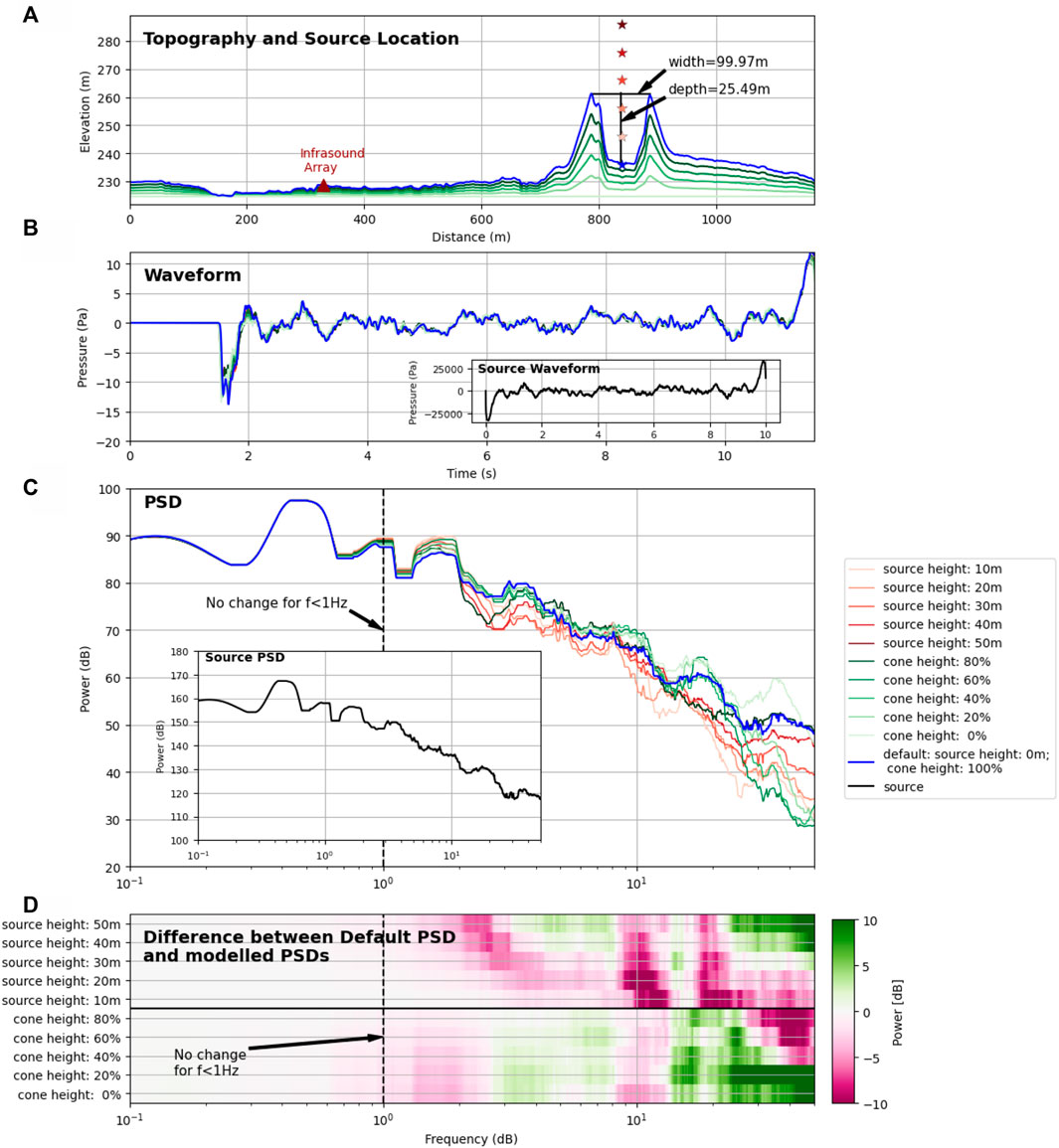
FIGURE 4. 3D acoustic propagation modeling setup and results. The colors in each subfigures follow the legend key on the right. (A) Topography along the direct path between active cone and infrasound array (red triangle). The different green and blue lines show the variation in topographic height as labeled in the legend. The stars show the variation of source heights used for the modeling. (B) Modeled waveforms at the location of the array. The source waveform is shown in the inset. (C) Power spectral density (PSD) of the waveforms in panel (B). The source PSD is shown in the inset. (D) Spectral difference between the varying setups and the default PSDs [from panel (C)]. Each horizontal line corresponds to the difference between the default PSD and the PSD with source height and topographic variations indicated on the left side y-axis. Green colors indicate a higher amplitude of the PSD with parameters on the left compared to the default whereas pink colors show lower amplitudes. The vertical dashed line at 1 Hz in (C,D) marks the approximate frequency below which we do not see any effect by the cone or source height.

We considered resonance of the cone as a potential infrasonic source, as this has been shown to be significant at Kīlauea (Fee et al., 2010a; Matoza et al., 2010) and other volcanoes (e.g., Johnson et al., 2018; Watson et al., 2020). The resonance frequency for a cavity with one open side can be estimated using f_R = c/(4L) ≈ 3.35 Hz. The resonance quality factor for volcanic craters can be defined as Q = 4L/(πa²) + 32L/(3π²a) (Moloney and Hatten, 2001; Johnson et al., 2018; Watson et al., 2020). For the geometry of the Ahu‘ailā‘au cone we get Q = 0.35, which is very low compared to other geometries such as in Villarica (Q ∼ 1–3 (Johnson et al., 2018)) or Etna (Q ∼ 2–5 Watson et al. (2020)). A low quality factor is indicative of inefficient trapping of resonant waves and strong radiation of energy into the atmosphere. We therefore do not expect any resonance of the cone to be a dominant source of the infrasound we observe.

Topographic features are known to diffract infrasonic waves and change the waveform significantly (e.g., Kim and Lees, 2011; Kim et al., 2015; Lacanna and Ripepe, 2020; Bishop et al., 2022). We conduct a first order analysis of topographic diffraction and propagation effects using the Finite Difference Time Domain code infraFDTD by Kim and Lees (2011). We use a 1.675 m spacial grid spacing and 0.0025 s time steps. Using the guideline of $>$10 nodes per wavelength (Hagness et al., 2005), we assume accurate frequency resolution up to 20 Hz. Since the DEM only shows the topography after the eruption, we assume that this is the maximum height of the cone as there are no reported collapse events after the eruption slowed down. Although the cone growth in Figure 3 is not symmetric, we analyze the influence of different cone heights by scaling the topography as shown in Figure 4A . Lava fountains are complex, with degassing and fragmentation happening at various locations and heights (Namiki et al., 2021). To investigate the influence of source location we vary the source height between 0 and 50 m above the bottom of the cone. We note that we only vary one parameter (cone height or source height) at a time and set the other parameter to their default, which is either the maximum topography or source height of 0 m. The source waveform is synthetically generated by taking the jet noise similarity spectra and inverse Fourier transforming the spectra to the time domain using random phases with a uniform distribution. The similarity spectra used for this was originally fitted to the infrasound PSD (Gestrich et al., 2021) and adjusted for the radial amplitude loss. The final source waveform has a duration of 10 s and is shown in blue in Figure 4B .

4.3 Jet noise scaling model

Fissure 8 produced a form of volcanic jet noise. Gestrich et al. (2021) developed a fitting method to automatically fit the similarity spectra to volcanic eruption data. They identified that the spectrum recorded from the eruption of fissure 8 fits the jet noise similarity spectra well. We perform a similar analysis for the entire fissure 8 time series and refer the reader to Gestrich et al. (2021) for details on the method. We calculate the root mean square deviation, the misfit between the LST and FST similarity spectra and every PSD calculated in Section 4.1.

Here, we introduce a method to estimate the jet velocity and diameter. We derive two main equations that use the acoustic parameters SPL (sound pressure level) and f_p (peak frequency) to invert for the volcanic jet parameters D_j (jet diameter) and v_j (jet velocity). To do this we first formulate the two base equations.

$10^{SPL/10}=\underset{\text{constant}}{\underbrace{k_1\left(c,r,\dots \right)}}{D}_j^2{v}_j^n(9)$

$f_p=\underset{\text{constant}}{\underbrace{k_2\left(S{t}_p\right)}}\frac{v_j}{D_j}.(10)$

These are adapted from Eqs 6, 8 and are expressed as functions that use jet parameters (diameter and velocity) to solve for acoustic parameters SPL (Eq. 9) and peak frequency (Eq. 10).

Since it is impossible to retrieve actual values for some of the volcanic jet paramters, we use ratios to express how the change in the infrasound parameters relate to the change in jet dynamics.

We use Eq. 9 and solve for the constant k₁ (Eq. 11). Assuming that the constants remain the same for the entire dataset, we know that the right side of Eq. 11 has to be the same for time t₀ and time t_i as shown in Eq. 12. Reorganizing and renaming variable ratios (Eq. 13) leads to Eq. 14, which relates the change in jet diameter, velocity, and SPL.

$k_1=10^{SPL/10}{D}_j^{-2}{v}_j^{-n}(11)$

$\Rightarrow 10^{SP{L}_0/10}{D}_{j,0}^{-2}{v}_{j,0}^{-n}=10^{SP{L}_i/10}{D}_{j,i}^{-2}{v}_{j,i}^{-n}(12)$

$\Rightarrow \underset{≔{\widehat{D}}^2}{\underbrace{\frac{D_{j,i}^{-2}}{D_{j,0}^{-2}}}}=\underset{≔\widehat{S}}{\underbrace{\frac{10^{SP{L}_i/10}}{10^{SP{L}_0/10}}}}\underset{≔{\widehat{v}}^{-n}}{\underbrace{\frac{v_{j,i}^{-n}}{v_{j,0}^{-n}}}}(13)$

$\Rightarrow \widehat{D}=\sqrt{\widehat{S}{\widehat{v}}^{-n}}\mathbf{o}\mathbf{r}:\widehat{v}={\left(\widehat{S}{\widehat{D}}^{-2}\right)}^{1/n}.(14)$

We then apply the same steps explained in the previous paragraph for Eq. 10 to derive Eq. 18, which relates the change in jet diameter, velocity, and peak frequency.

$k_2=\frac{f_p{D}_j}{v_j}(15)$

$\Rightarrow \frac{f_{p,0}{D}_{j,0}}{v_{j,0}}=\frac{f_{p,i}{D}_{j,i}}{v_{j,i}}(16)$

$\Rightarrow \underset{≔\widehat{D}}{\underbrace{\frac{D_{j,i}}{D_{j,0}}}}=\underset{≔{\widehat{f}}^{-1}}{\underbrace{\frac{f_{p,0}}{f_{p,i}}}}\underset{≔\widehat{v}}{\underbrace{\frac{v_{j,i}}{v_{j,0}}}}(17)$

$\Rightarrow \widehat{D}=\widehat{v}{\widehat{f}}^{-1}\mathbf{o}\mathbf{r}:\widehat{v}=\widehat{D}\widehat{f}(18)$

In summary, the ratios for the jet diameter, velocity, frequency, and SPL number are now:

$\widehat{D}=\frac{D_{j,i}}{D_{j,0}}(19)$

$\widehat{v}=\frac{v_{j,i}}{v_{j,0}}(20)$

$\widehat{f}=\frac{f_{p,i}}{f_{p,0}}(21)$

$\widehat{S}=\frac{10^{SP{L}_i/10}}{10^{SP{L}_0/10}}(22)$

Eqs 14, 18 have to be true and solvable with the same parameter set. Therefore we first set Eqs 14, 18 equal with regards to the diameter ratio and solve for the velocity ratio:

$\sqrt{\widehat{S}{\widehat{v}}^{-n}}=\widehat{v}{\widehat{f}}^{-1}(23)$

$\iff \widehat{v}={\left(\widehat{S}\widehat{f}\right)}^{\frac{1}{n+2}}(24)$

And secondly we set Eqs 14, 18 equal with regards to the velocity ratio and solve for the diameter ratio:

${\left(\widehat{S}{\widehat{D}}^{-2}\right)}^{1/n}=\widehat{D}\widehat{f}(25)$

$\iff \widehat{D}={\left(\widehat{f}{\widehat{S}}^{-1/n}\right)}^{-\frac{n}{n+2}}(26)$

Eqs 24, 26 are now equations that relate the change in SPL and peak frequency to a change in jet velocity and jet diameter. Due to our $\sim 90°$ observations angle we assume values for n_I are between 5 and 8 (Matoza et al., 2013).

5 Results

5.1 UAS observations

In Figure 2, we show eight single video frames taken on different days to show representative activity from each video. In the beginning of June the videos show 1 – 3 relatively tall lava fountains ejected from the fissure 8 vent (see June 2–3 in Figure 2 and Supplementary Video S1). These fountains have a center of variably coherent, porous magma and already liberated gas. The pyroclasts are decelerated by gravitational forces until they reverse direction and fall down outside of the central core. This makes it difficult to identify the diameter of the central core. The height of the fountain fluctuates within a couple of meters over very short time scales (2–6 s). In the UAS videos the falling pyroclasts obscure the view of the central core and the dynamics of the outflow or potential ponding. However, it is clear that the spatter of the fountains leads to the growth of the cone surrounding the fountain (Figure 3). The DEM shows that by the end of the eruption the cone measured approximately 25 m in depth and 100 m in diameter. Note that the depth is measured after the eruption, when lava had ponded and solidified in the cone or partially drained out.

UAS videos of June 9–10 show an apparent slight decrease in fountain height and growth in cone height, with the fountain height still being taller than the cone height (see Figure 2 and Supplementary Video S2). The fountain is broader and less distinct and seems to occupy a larger area of the cone center. The profile of the cone growth is shown in Figure 3. After June 16 the videos show that the fountain height is significantly lower, not reaching over the cone top (see Figure 2; Supplementary Videos S3,S4). With a fountain lower than the cone, we assume that the cone did not significantly gain in height after this time. The activity could be described as a roaring lava pond that is highly turbulent, with lava being splashed against the inner sides of the cone. It is clear that the entirety of the inner cone is churning and overturning. Anecdotes describe a “drowning fountain”, which indicates a rise of the ponding and decrease of fountain height. However, it is difficult to see whether the pond height has increased in the videos.

Interestingly, the fountain height, which continuously decreased in height between the beginning of June to the end of June, does not seem to correlate with the discharge rates determined by Dietterich et al. (2021), which peaked on June 16, and Plank et al. (2021), which peaked between June 9–19.

5.2 Infrasound

Array processing shows that fissure 8 is the dominant infrasound source during the study period. The median cross correlation maxima (MdCCM) calculations in Figure 1B show very high correlation values throughout the study period, with the backazimuth centered around the median of 121.7° for the time before the pulses start. This backazimuth coincides with the lowest point of the fissure, which is centered in the surrounding cone. The maximum extent of backazimuth fluctuations before the pulses is between approximately 119° and 125°, which is still inside the cone. Since these values correspond to the backazimuth that produces the highest correlation, we interpret these results as that the highest coherent acoustic energy comes from the fissure itself. With the start of the pulses after July 14, the backazimuth results are more scattered and pointing intermittently to lower backazimuth angles, which is consistent with the interpretation by Lyons et al. (2021) that associates the lower backazimuths with increased activity in the spillway during the pulses.

The waveforms, shown as beamformed signal in Figure 5A, are dominated by a continuous signal from the volcano without showing signs of distinct explosions or notable short-term (seconds to minutes) deviations in the amplitudes. The amplitude distribution can be expressed in skewness with a positive skewness meaning that most of the waveform having positive pressure values. Opposed to supersonic jets that show a positive waveform skewness of up to ∼3.5 in Fee et al. (2013), the eruption of fissure 8 does not show significant skewness (values $<$0.15), which is consistent with subsonic jetting (see Supplementary Figure S1).

FIGURE 5

FIGURE 5. Overview of infrasound properties. (A) Shows the beamformed waveform using all four infrasound microphones, (B) the spectrogram and 10 h rolling mean peak frequency in purple and (C) shows the calculated 10 h rolling mean sound pressure level (SPL) for different frequency bands labeled in the legend. The background colors are the same as in Figure 1.

In Figure 5B we show all calculated PSDs as a spectrogram as well as the 10 h rolling mean peak frequency as a purple line. Here, the peak frequency is the frequency of highest PSD amplitude between 0.2 and 10 Hz. We choose this frequency range because frequencies below 0.2 Hz can be highly influenced by wind as shown in the Supplementary Figure S2 and (Fee and Garcés, 2007). Above approximately 3 Hz the spectral amplitude steadily declines toward higher frequencies and we choose an upper bound of 10 Hz. This frequency range encompasses the majority of the acoustic signal and allows characterization of the spectral slope (Matoza et al., 2009; Gestrich et al., 2021). Generally the spectrum is stable over the study period. The peak frequency in Figure 5B is ∼ 0.7–1 Hz before mid-June (June 16; marked with a dashed line and different background colors) and then declines to approximately 0.3 Hz. This change is not as sudden as it seems in the plot, but rather represents the transition of peak frequency from a steady decline of the frequencies around 0.7–1 Hz and increase of frequencies around 0.3 Hz. The frequency drop in Figure 5B represents when the lower frequencies dominate the higher frequencies. This change is also apparent in Figure 6 where the blue line shows the median PSD in the first time window (until mid-June) and the red line shows the median PSD for the second time window (mid-June to mid-July). The earlier PSD shape has its maximum around 1 Hz and the later PSD’s maximum is around 0.3 Hz.

FIGURE 6

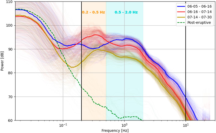
FIGURE 6. Power Spectral Density (PSD) curves colored according to different time windows as labeled in the legend. Note that the colors also correspond to the time windows shown in Figures 1, 5, 7, 8. The thin lines are every calculated PSD and the thick lines are showing the median PSD for the whole time window. The black vertical lines outline the overall frequency band of interest (0.2–10 Hz) and the orange and light blue background panels show the frequency bands that are also used in Figure 5C for the calculation of SPL.

It is apparent in Figure 5A that the amplitudes of the waveforms rises before peaking in mid-June (June 16) and then steadily declining until mid-July. To further quantify the amplitude evolution we calculate the 10 h rolling mean SPL between 0.2 and 10 Hz (black line in Figure 5C). It confirms that the SPL in this frequency band rises by about 4 dB in the first 12 days of recording and then declines by almost 10 dB until mid-July. We also calculate the SPL for two different frequency bands, both according to the peaks before (0.5–2 Hz) and after mid-June (0.2–0.5 Hz) as shown in Figure 6. One can see that the SPL of the upper frequency band (0.5–2 Hz) has a very similar time evolution as the overall SPL (0.2–10 Hz). In contrast, the lower frequency band (0.2–0.5 Hz) is first lower in SPL than the upper frequency band but surpasses exactly at the time that the overall and upper frequency band SPL peak (June 16) before it peaks about 3 days later. This shows that the sudden drop in frequency observed in Figure 5B only corresponds to the time when the lower frequency band has a higher SPL than the upper frequency band, which is a gradual change.

5.3 Topographic effects

The FDTD modeling results show that there is no significant influence of the cone or source height for frequencies below 1.5 Hz. The waveforms computed for the different model setups at the location of the infrasound array (see Figure 4B) are used to calculate each power spectral density (PSD) shown in Figure 4C . To emphasize the influence of topography and source height we calculate the difference between the PSD of the default model setup (full topography and source at no elevation) and the PSDs with varying setups as shown in Figure 4D . Our modeling only predicts major amplitude deviations for frequencies $>$1 Hz with increases in amplitude (green color in Figure 4D) or decreases in amplitude (pink color in Figure 4D). There are some trends such as a decrease of approximately 10 dB at 10 Hz for higher source heights and an increase of amplitude of more than 10 dB above 20 Hz for very low cone heights. The deviations are generally at frequencies higher than the peak frequency calculated in Section 5.2.

5.4 Jet noise fitting

The jet noise fitting shows good agreement between the jet noise similarity spectra and the recorded infrasound. The overall misfit is calculated for the frequency band of 0.2–10 Hz to stay consistent with the infrasound processing in Section 4.1. Note that these are different bounds compared to those used in Gestrich et al. (2021). The peak frequency is bound between 0.15 and 8 Hz. The misfit difference spectrogram is calculated using 20 overlapping frequency bands within the bounds 0.2–10 Hz with logarithmic width so that the highest frequency of each individual frequency band is ten times the lowest frequency. Figure 7A shows the result of the overall fitting and we observe very low misfit values, similar to Gestrich et al. (2021). After June 16 the LST misfit is slightly lower. The misfit difference spectrogram in Figure 7B also shows a better fit of the FST similarity spectrum after June 16 for almost the entire frequency band. The better fit with the FST similarity spectrum is due to its slightly wider shape as shown in Figure 6. Also, the lower frequency bound of 0.2 Hz is above the local minima which is at approximately 0.1 Hz and therefore the fitting misses the left side of the similarity spectra. We show in the Supplementary Figure S3 the result when fitting between 0.1 and 10 Hz, which is slightly more scattered but in general very similar to Figure 7.

FIGURE 7

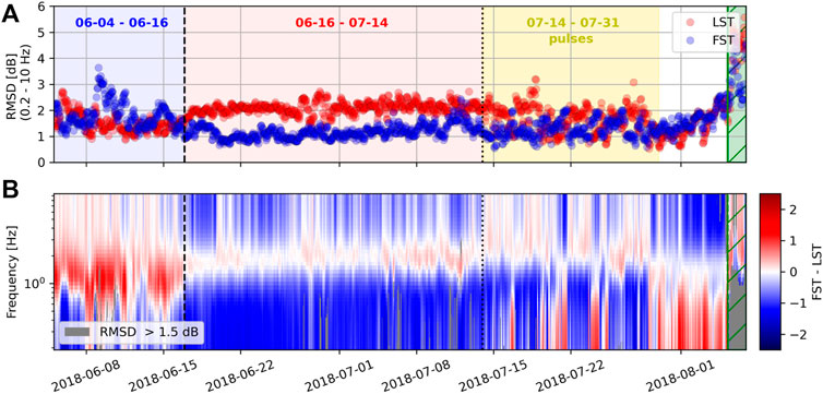
FIGURE 7. Jet noise similarity spectra fitting results. (A) Shows the misfit (RMSD) when fitting the LST (red) and FST (blue) similarity spectra to the power spectra shown in Figure 5B. With the RMSD being generally below three the similarity spectra fit the eruption data well. (B) Shows the misfit difference spectrogram with red marking times and frequencies where the LST similarity spectrum fits the data better and in blue when the FST similarity spectrum fits the data better. The background colors and vertical dashed and dotted lines are the same as in Figure 1.

5.5 Jet noise scaling model

First, we calculate the SPL ratio $\widehat{S}$ (Eq. 22) and peak frequency ratio $\widehat{f}$ (Eq. 21) using the 10 h rolling mean of the SPL and peak frequency shown in Figures 5B,C as time series SPL_i and f_p,i. As a reference SPL, SPL₀, and peak frequency, f_p,0 we calculate the mean SPL and peak frequency values for the first 2 days of recording before June 7, which are SPL₀ = 94.29 dB and f_p,0 = 0.86 Hz. The resulting ratios using Eqs. 22, 21 are shown in Figure 8A and are the input parameters for the scaling relationships expressed in Eqs 24, 26. The results are shown in Figure 8B. Before June 16, both the velocity and jet diameter ratio vary but generally stay around $\widehat{v}\sim$1 and $\widehat{D}\sim$1. After June 16 the diameter ratio increases up to $\widehat{D}\sim$2.5 and stays around $\widehat{D}\sim$2.3 for the rest of June, which suggests that the volcanic jet diameter has more than doubled since the beginning of June. The diameter ratio slightly decreases in the beginning of July to around 1.1 $\widehat{D}\sim$1.8. The velocity ratio shows an opposite trend as it drops on June 16 to $\widehat{v}\sim$0.85, which is 85% of the velocity in the beginning of June, and continues to slowly decrease down to $\widehat{v}\sim$0.7 until mid-July.

FIGURE 8

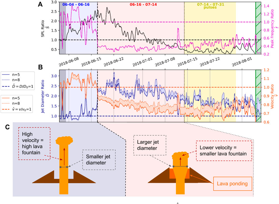
FIGURE 8. Jet noise scaling model results. (A) Shows the SPL ratio $\widehat{S}$ as a black line with amplitudes on the left y-axis and peak frequency ratio $\widehat{f}$ in magenta with amplitude values on the right y-axis. (B) Shows the model results. The dark grey panel in the beginning of the time series shows the time window used to calculate the initial parameters SPL₀ and f₀ used to calculate the input parameter ratios. The dark blue lines show the change of jet diameter ratio with time with the solid line showing the minimum velocity exponent of n = 5 and the dotted line the maximum assumed velocity exponent of n = 8. Values for the diameter ratio are shown on the left y-axis and D/D₀ = 1 is marked with a horizontal dashed blue line. The orange lines show the change of velocity ratio with values on the right y-axis and line styles like the diameter ratio which are also labeled in the legend. The background colors and vertical dashed and dotted lines are the same as in Figure 1. (C) shows a sketch illustrating the interpretation of the modelling results with background colors indicating the time window the sketch is corresponding to. On the left, the initial high velocity and low jet diameter is interpreted as a tall narrow fountain. On the right the decrease in velocity and increase in jet diameter is interpreted as a decrease in fountain height and increase in fountain diameter, potentially due to the evolving pond.

The uncertainty in the velocity exponent n = 5 to 8 leads to variations in the velocity ratio of up to 0.1 and for the diameter ratio up to 0.3 but does not change the overall observed trend of both ratios.

6 Discussion

Infrasound-derived inferences on the lava fountain dynamics are consistent with those derived from UAS video footage. First, the waveforms and spectra for the entirety of the study period are consistent with jetting (Figure 7, Section 5.4). The UAS video footage and infrasound recordings show a change in parameters around mid-June. Generally, the lava fountain went from a high, distinct fountain in late May and early June to a low, broad fountain within a lava pond around mid-June (Figure 2). This coincides with the maximum SPL and a notable drop in peak frequency (Figure 1B). To quantify which changes in the jet dynamics could be responsible for the high SPL and drop in peak frequency we apply jet noise scaling relationships in Section 5.5. The results show that the change of SPL and peak frequency from June 16 on are correlated with a jet velocity decrease and jet diameter increase illustrated in a sketch in Figure 8C. As the jet velocity decrease coincides with the lava fountain height decrease observed in the UAS data, we hypothesize that the lava clast velocity is roughly proportional to the gas velocity. Using the simple ballistic equation from Section 2.1, we can derive the lava fountain height ratio and jet velocity via: $\widehat{H}=\frac{H}{H_0}={\left(\frac{v}{v_0}\right)}^2={\widehat{v}}^2$. With an initial velocity drop around mid-June to $\widehat{v}\sim 0.85$ (see Figure 8 and Section 5.5), this would translate to a drop of fountain height by a factor of $\widehat{H}\sim 0.72$. This means that the fountain height in mid-June is about 30% less high than in the beginning of June. By the beginning of July the velocity dropped to approximately $\widehat{v}\sim 0.7$, which corresponds to a fountain height reduction to 49% of the initial height in the beginning of June. These calculations qualitatively agree with UAS video footage (Figure 2).

The increased infrasound amplitudes could be produced through an increase in jet diameter, which would also produce a decrease in peak frequency. The increase in jet diameter can be explained by an increase in vent diameter via erosion, which is likely during sustained fissure eruptions Parcheta et al. (2015). Another way to achieve a larger subaerial jet diameter is through the entrainment of lava from the pond, leading to a reduction in jet velocity (Wilson et al., 1995). The potential ponding of lava in the cone that grew in the first half on June could have led to a decrease in fountain height while producing higher lava and SO₂ discharge rates. These discharge rates peak in mid June and stay relatively high for the next month (e.g., Dietterich et al., 2021; Lerner et al., 2021). Suppression of the fountain height through ponding would also match the anecdotal descriptions of a “drowning fountain” by local observers. Ponding-related decrease in fountain height has been reported in past eruptions of Kīlauea volcano, such as the 1959 Kīlauea Iki eruption (Richter et al., 1970) and the 1961 Halema’uma’u eruption (Richter et al., 1964), as well as the 2014/15 Holuhraun, Iceland, eruption (Witt et al., 2018). The deceleration of the magma-gas mixture matches with the calculated decrease in gas velocity in Figure 8.

We note that the presence of multiple fountains in the beginning of June (Figure 2) would likely not have a significant effect on our modeling results. For simplicity our jet noise scaling model only considers a single fountain as we are unable to know exactly at which point in time there were multiple fountains and how their relative dynamics changed as we do not have continuous video observations. Some of the videos before June 16 show two fountains with one fountain being 2–3 times as high as the other fountain. At the most we can distinguish three fountains on June 10. We assume the phase of the signal emitted by each fountain is incoherent which leads to partially destructive interference and partially constructive interference and the addition of amplitude similar to incoherent addition explained in Papamoschou (2013) and Supplementary Section S1.3. As shown in Supplementary Section S1.3; Supplementary Figure S4, we suggest the presence of three equal strength fountains could cause a deviation in jet velocity and jet diameter ratio of up to 15%. However, this effect may be viewed as an upper bound as we mostly observe one dominant fountain with one or more much smaller fountains. For example, assuming the secondary fountain produces less than half of the acoustic pressure produced by the main fountain, the inferred change in jet ratio would be below 3%. Future work is needed to obtain a more detailed view on the influence of multiple fountains on acoustic recordings.

We also acknowledge the possibility that the lava fountain and the turbulent lava pond jetting are two separate, but potentially connected, volcanic jet noise sources. The existence of multiple sources during volcanic eruptions has been previously proposed by Matoza et al. (2009) and Fee et al. (2010a). One possible interpretation is that at the beginning of the eruption the lava fountain produces relatively higher frequency jet noise due to its smaller jet diameter. With the decrease in fountain height the jet velocity also decreases, which leads to a decrease in acoustic power and amplitude. At the same time, the turbulence and vigorous degassing of the lava pond turbulence could already be producing a low frequency jet noise. The lava pond does not exist at the beginning of the eruption and grows slowly during the cone build-up in early June. As the pond grows, the lava fountain momentum is decreased due to the entrainment and interaction with the pond, while the lava pond becomes more and more turbulent. The increased pond turbulence may increase the acoustic power from the pond and eventually become dominant over the fountain jetting. The spectrogram, SPL and PSDs in Figures 5, 6 may support this hypothesis, as the change in peak frequency in mid-June is a result of the amplitude decrease of the broad spectral peak around 1 Hz and amplitude increase of the spectral peak around 0.3 Hz, rather than a gradual move of the peak frequency as explained in Section 5.2. The good fit of the jet noise similarity spectra with the observed infrasonic spectra throughout the eruption supports the assumption that the dominant acoustic source is jet noise. The distinction whether there is one jet source that is changing or two jet sources (the fountain and lava pond) that change in relative intensity is not possible here as they would both originate from essentially the same location. Controlled experiments or numerical models are needed to discriminate the acoustic effects.

The good correlation between the observed eruption dynamics and the infrasonic jet noise model results presented here suggests that jet noise scaling laws are applicable to sustained lava fountains and can provide a first order approximation of changes in lava fountain dimensions and dynamics. However, jet noise scaling laws used in this analysis were originally derived for laboratory-scale, gas-only jets. Lava fountains consists of multiple phases such as melt clods and rock fragments. It is unclear how the partially solid and liquid phases of the lava fountain influence the radiated acoustic amplitude. There is limited available literature on the effects of particles and multiple phases in jet noise. Analysis and experiments by Kandula (2008) showed that water injection in a jet reduces the jet noise acoustic amplitude. However, the water droplets in that study were very small and the injection decreased the jet temperature through evaporation. Based on Kandula (2008), liquids could potentially decrease the volcanic jet noise, although we note in the case of volcanoes with hot gas, solids, and liquid rock this effect could be different. The effect of these phases on the jet noise should be investigated in the future. Additionally, the very hot gas temperature during lava flow and most volcanic eruptions also has an effect on the velocity exponent as investigated by Viswanathan (2006). Namiki et al. (2021) measured temperatures up to 1,000°C, and Gansecki et al. (2019) reported temperatures up to 1,150°C for the erupting fissure 8 lava fountain. Even assuming just a moderately high temperature in the immediate vicinity of the lava fountain of ca. 200–400°C (Namiki et al., 2021), the temperature ratio is between 2.5 and 5.75, which is at the higher end or even higher than investigated by Viswanathan (2006). Additionally, the velocity exponent is dependent on the angle to the center jet axis. Our infrasound array observations are made from a single location at approximately 90° from the jet axis. With those two assumptions, the velocity exponent for the acoustic intensity may be below 6.

A decrease in velocity and Mach number could explain the change in jet noise spectral fitting after mid-June. We cannot determine absolute values for the Mach numbers during this eruption, but since Ma = v/c, the change in velocity observed in our model results, as well as in the video observations, would correspond to the same change in Mach number. This assumes that the temperature, and therefore speed of sound c, does not change. As discussed in Section 5.4 we observe that the spectrum is best fit by the narrower LST spectrum the first half of June, and then after mid-June the spectra more closely resembles FST noise (Figure 7). In general, at an observation angle of 90° the FST noise is expected to be dominant (Tam et al., 2008). However, other volcano studies such as Matoza et al. (2009) and Gestrich et al. (2021) have previously observed a better fit of the LST similarity spectrum as opposed to the FST spectrum when compared to some volcanic eruptions. Tam et al. (2008) showed that the LST dominant cone becomes wider with an increased Mach number and jet temperature ratio. For high temperature ratios (2.2 used in Tam et al. (2008)) the LST jet noise is dominant above approximately 120° for M=1, which is the upper limit of considered Mach numbers since we assume subsonic conditions as explained before. With decreasing Mach number the LST dominated cone becomes more narrow and dominated for observation angles above approximately 130° for M=0.6. Tam et al. (2008) additionally noted a temperature dependence with a widening of the LST cone to lower angles as the temperature ratio increases. Since the temperature ratio is possibly even higher than the 2.2 used by Tam et al. (2008), as discussed in the previous paragraph, LST jet noise may be produced at our observation angle of approximately 90° at the beginning of the eruption when the jet velocity is high (see Figure 7) and then changes to be FST dominant when the jet velocity decreases in mid-June. Further laboratory experiments at higher temperature ratios and the addition of solids and liquids are needed to investigate the decrease in Mach number with the change in jet noise spectral shape during volcanic eruptions at an observation angle of 90°.

7 Conclusion

Our study connects observed lava fountain dynamics with recorded infrasound signals using jet noise scaling relationships. The eruption of fissure 8, Kīlauea volcano in 2018 produced a sustained lava fountain over a period of months and constructed the cone, Ahu‘ailā‘au. Uncrewed Aircraft Systems (UAS) video footage revealed a change in fountain height as well as a change in dynamics from a tall, distinct fountain to a lower, broad fountain feeding a lava lake. The sound from the lava fountain was recorded by a nearby infrasound array, and the sound qualitatively and quantitatively resembles the sound produced by jet engines. Analysis of the infrasound reveals a clear change in peak frequency and sound pressure level over the course of June 2018. We develop a model based on jet noise relationships that calculates the relative change in volcanic jet diameter and velocity using infrasound sound pressure level and peak frequency. The decrease in peak frequency and increase in sound pressure level correspond with a broadening of fountain width and decrease in fountain height. The good match between the modeled change of jet diameter and velocity compared to the observed lava fountain dynamics suggests that the predominant noise source is turbulence and that the jet noise scaling relationships can be used to estimate changes in lava fountain dimensions. Because the jet noise scaling equations are based on gas-only laboratory jets, we have yet to determine the influence of the liquid and solid phases and extreme temperatures on the scaling of amplitude and frequency as well as spectral shape of the infrasound recordings. We suggest controlled laboratory experiments or numerical analysis to further investigate these factors.

Data availability statement

The infrasound data recorded during the eruption of Kīlauea’s fissure 8 are publicly available at the IRIS DMC with network code 5L and station name FIS8 (at http://ds.iris.edu/mda/5L/). The DEM used in this study can be found in the USGS data base https://www.sciencebase.gov/catalog/item/5eb19f3882cefae35a29c363. The UAS data can be found in the USGS data base https://www.sciencebase.gov/catalog/item/5ea8b45482cefae35a1faf94.

Author contributions

JG performed the analysis of the dataset. JG, DF, and RM developed the jet noise model. JG and DF wrote the manuscript. JL, HD, MP, and CP helped with the data collection and on-site observations. JG, DF, RM, JL, HD, VC, and UK contributed with the interpretation of the data analysis.

Funding

JG and DF acknowledge funding from NSF Grant EAR-1901614. RM acknowledges NSF grant EAR-1847736. VC acknowledges funding from Deutsche Forschungsgemeinschaft project CI306/2–1.

Acknowledgments

Data collection was facilitated by members of the United States Geological Survey’s Hawaiian Volcano Observatory as well as the United States Geological Survey’s Alaska Volcano Observatory. The majority of the analysis was done at the University of Alaska Fairbanks, located on the ancestral land of the Dena people of the lower Tanana River. We acknowledge that our field work took place in the ahupua‘a of Keauhou and Kapapala, in the moku of Ka‘ū, on the mokupuni of Hawai‘i, which are the ancestral, traditional, and contemporary lands of the Native Hawaiian people. We want to thank Karoly Nemeth and Jacopo Taddeucci for their thorough revisions. Carl Tape, Oliver Lamb and Valerie Wasser provided helpful comments. Any use of trade, firm, or product names is for descriptive purposes only and does not imply endorsement by the United States Government.

Conflict of interest

The authors declare that the research was conducted in the absence of any commercial or financial relationships that could be construed as a potential conflict of interest.

Publisher’s note

All claims expressed in this article are solely those of the authors and do not necessarily represent those of their affiliated organizations, or those of the publisher, the editors and the reviewers. Any product that may be evaluated in this article, or claim that may be made by its manufacturer, is not guaranteed or endorsed by the publisher.

Supplementary material

The Supplementary Material for this article can be found online at: https://www.frontiersin.org/articles/10.3389/feart.2022.1027408/full#supplementary-material

References

Anderson, K. R., Johanson, I. A., Patrick, M. R., Gu, M., Segall, P., Poland, M. P., et al. (2019). Magma reservoir failure and the onset of caldera collapse at Kīlauea Volcano in 2018. Science 366, eaaz1822. doi:10.1126/science.aaz1822

PubMed Abstract | CrossRef Full Text | Google Scholar

Bishop, J. W., Fee, D., Modrak, R., Tape, C., and Kim, K. (2022). Spectral element modeling of acoustic to seismic coupling over topography. JGR. Solid Earth 127. doi:10.1029/2021JB023142

CrossRef Full Text | Google Scholar

Bishop, J. W., Fee, D., and Szuberla, C. A. (2020). Improved infrasound array processing with robust estimators. Geophys. J. Int. 221, 2058–2074. doi:10.1093/GJI/GGAA110

CrossRef Full Text | Google Scholar

Dabrowa, A. L., Green, D. N., Rust, A. C., and Phillips, J. C. (2011). A global study of volcanic infrasound characteristics and the potential for long-range monitoring. Earth Planet. Sci. Lett. 310, 369–379. doi:10.1016/j.epsl.2011.08.027

CrossRef Full Text | Google Scholar

DeSmither, L., Diefenbach, A., and Dietterich, H. (2021). Unoccupied aircraft systems (uas) video of the 2018 lower east rift zone eruption of Kīlauea volcano. hawaii: Data Release. doi:10.5066/P9BVENTG

CrossRef Full Text | Google Scholar

Dietterich, H. R., Diefenbach, A. K., Soule, S. A., Zoeller, M. H., Patrick, M. R., Major, J. J., et al. (2021). Lava effusion rate evolution and erupted volume during the 2018 Kīlauea lower East Rift Zone eruption. Bull. Volcanol. 83, 25. doi:10.1007/s00445-021-01443-6

CrossRef Full Text | Google Scholar

Evans, B. M., and Staudacher, T. H. (2001). In situ measurements of gas discharges across fissures associated with lava flows at Réunion Island. J. Volcanol. Geotherm. Res. 106, 255–263. doi:10.1016/S0377-0273(00)00242-0

CrossRef Full Text | Google Scholar

Fee, D., and Garcés, M. (2007). Infrasonic tremor in the diffraction zone. Geophys. Res. Lett. 34, 1–5. doi:10.1029/2007GL030616

CrossRef Full Text | Google Scholar

Fee, D., Garces, M., Orr, T., and Poland, M. (2011). Infrasound from the 2007 fissure eruptions of Kīlauea volcano, hawai’i. Geophys. Res. Lett. 38, 1–5. doi:10.1029/2010GL046422

CrossRef Full Text | Google Scholar

Fee, D., Garcés, M., Patrick, M. R., Chouet, B., Dawson, P., and Swanson, D. (2010a). Infrasonic harmonic tremor and degassing bursts from Halema’uma’u Crater, Kīlauea Volcano, Hawaii. J. Geophys. Res. 115, 113166. doi:10.1029/2010JB007642

CrossRef Full Text | Google Scholar

Fee, D., Haney, M. M., Matoza, R. S., Van Eaton, A. R., Cervelli, P., Schneider, D. J., et al. (2017). Volcanic tremor and plume height hysteresis from Pavlof Volcano, Alaska. Science 355, 45–48. doi:10.1126/science.aah6108

PubMed Abstract | CrossRef Full Text | Google Scholar

Fee, D., and Matoza, R. S. (2013). An overview of volcano infrasound: From Hawaiian to plinian, local to global. J. Volcanol. Geotherm. Res. 249, 123–139. doi:10.1016/j.jvolgeores.2012.09.002

CrossRef Full Text | Google Scholar

Fee, D., Matoza, R. S., Gee, K. L., Neilsen, T. B., and Ogden, D. E. (2013). Infrasonic crackle and supersonic jet noise from the eruption of Nabro Volcano, Eritrea. Geophys. Res. Lett. 40, 4199–4203. doi:10.1002/grl.50827

CrossRef Full Text | Google Scholar

Fee, D., Steffke, A., and Garces, M. (2010b). Characterization of the 2008 Kasatochi and Okmok eruptions using remote infrasound arrays. J. Geophys. Res. 115, D00L10–15. doi:10.1029/2009JD013621

CrossRef Full Text | Google Scholar

Fernández, J. J. P., and Sesterhenn, J. (2017). Compressible starting jet: Pinch-off and vortex ring-trailing jet interaction. J. Fluid Mech. 817, 560–589. doi:10.1017/jfm.2017.128

CrossRef Full Text | Google Scholar

Gansecki, C., Lopaka Lee, R., Shea, T., Lundblad, S. P., Hon, K., and Parcheta, C. (2019). The tangled tale of Kīlauea’s 2018 eruption as told by geochemical monitoring. Science 366, eaaz0147. doi:10.1126/science.aaz0147

PubMed Abstract | CrossRef Full Text | Google Scholar

Garcés, M. A., Fee, D., and Matoza, R. S. (2013). Volcano acoustics. Model. Volcan. Process. Phys. Math. Volcanism 9780521895, 359–383. doi:10.1017/CBO9781139021562.016

CrossRef Full Text | Google Scholar

Gestrich, J. E., Fee, D., Matoza, R. S., Lyons, J. J., and Ruiz, M. C. (2021). Fitting jet noise similarity spectra to Volcano infrasound data. Earth Space Sci. 8, 1–16. doi:10.1029/2021ea001894

CrossRef Full Text | Google Scholar

Gonnermann, H. M., and Manga, M. (2007). The fluid mechanics inside a volcano. Annu. Rev. Fluid Mech. 39, 321–356. doi:10.1146/annurev.fluid.39.050905.110207

CrossRef Full Text | Google Scholar

Hagness, S. C., Taflove, A., and Gedney, S. D. (2005). Finite-difference time-domain methods. Numer. Methods Electromagn. Handb. Numer. Analysis 13, 199–315. doi:10.1016/S1570-8659(04)13003-2

CrossRef Full Text | Google Scholar

Haney, M. M., Matoza, R. S., Fee, D., and Aldridge, D. F. (2018). Seismic equivalents of volcanic jet scaling laws and multipoles in acoustics. Geophys. J. Int. 213, 623–636. doi:10.1093/gji/ggx554

CrossRef Full Text | Google Scholar

Houghton, B. F., Cockshell, W. A., Gregg, C. E., Walker, B. H., Kim, K., Tisdale, C. M., et al. (2021). Land, lava, and disaster create a social dilemma after the 2018 eruption of Kīlauea volcano. Nat. Commun. 12, 1223. doi:10.1038/s41467-021-21455-2

PubMed Abstract | CrossRef Full Text | Google Scholar

Iezzi, A. M., Fee, D., Kim, K., Jolly, A. D., and Matoza, R. S. (2019). Three-dimensional acoustic multipole waveform inversion at yasur volcano, Vanuatu. J. Geophys. Res. Solid Earth 124, 8679–8703. doi:10.1029/2018JB017073

CrossRef Full Text | Google Scholar

Johnson, J. B., and Miller, A. J. (2014). Application of the monopole source to quantify explosive flux during vulcanian explosions at Sakurajima Volcano (Japan). Seismol. Res. Lett. 85, 1163–1176. doi:10.1785/0220140058

CrossRef Full Text | Google Scholar

Johnson, J. B., Watson, L. M., Palma, J. L., Dunham, E. M., and Anderson, J. F. (2018). Forecasting the eruption of an open-vent volcano using resonant infrasound tones. Geophys. Res. Lett. 45, 2213–2220. doi:10.1002/2017GL076506

CrossRef Full Text | Google Scholar

Kandula, M. (2008). Prediction of turbulent jet mixing noise reduction by water injection. AIAA J. 46, 2714–2722. doi:10.2514/1.33599

CrossRef Full Text | Google Scholar

Kern, C., Lerner, A. H., Elias, T., Nadeau, P. A., Holland, L., Kelly, P. J., et al. (2020). Quantifying gas emissions associated with the 2018 rift eruption of Kīlauea Volcano using ground-based DOAS measurements. Bull. Volcanol. 82, 55. doi:10.1007/s00445-020-01390-8

CrossRef Full Text | Google Scholar

Kieffer, S. W., and Sturtevant, B. (1984). Laboratory studies of volcanic jets. J. Geophys. Res. 89, 8253–8268. doi:10.1029/jb089ib10p08253

CrossRef Full Text | Google Scholar

Kim, K., Fee, D., Yokoo, A., and Lees, J. M. (2015). Acoustic source inversion to estimate volume flux from volcanic explosions. Geophys. Res. Lett. 42, 5243–5249. doi:10.1002/2015GL064466

CrossRef Full Text | Google Scholar

Kim, K., and Lees, J. M. (2011). Finite-difference time-domain modeling of transient infrasonic wavefields excited by volcanic explosions. Geophys. Res. Lett. 38, 2–6. doi:10.1029/2010GL046615

CrossRef Full Text | Google Scholar

Lacanna, G., and Ripepe, M. (2020). Modeling the acoustic flux inside the magmatic conduit by 3D-FDTD simulation. J. Geophys. Res. Solid Earth 125, 1–18. doi:10.1029/2019JB018849

CrossRef Full Text | Google Scholar

Lamb, O. D., Gestrich, J. E., Barnie, T. D., Ducrocq, C., Shore, M. J., Lees, J. M., et al. (2022). Acoustic observations of lava fountain activity during the 2021 Fagradalsfjall eruption, Iceland. Bull. Volcanol. 84, 96–18. doi:10.1007/s00445-022-01602-3

CrossRef Full Text | Google Scholar

Lerner, A. H., Wallace, P. J., Shea, T., Mourey, A. J., Kelly, P. J., Nadeau, P. A., et al. (2021). The petrologic and degassing behavior of sulfur and other magmatic volatiles from the 2018 eruption of Kīlauea, Hawai‘i: Melt concentrations, magma storage depths, and magma recycling. Bull. Volcanol. 83, 43. doi:10.1007/s00445-021-01459-y

CrossRef Full Text | Google Scholar

Lyons, J. J., Dietterich, H. R., Patrick, M. P., and Fee, D. (2021). High - speed lava flow infrasound from Kīlauea ’ s fissure 8 and its utility in monitoring effusion rate. Bull. Volcanol. 83, 66. doi:10.1007/s00445-021-01488-7

CrossRef Full Text | Google Scholar

Mathews, L. T., Gee, K. L., and Hart, G. W. (2021). Characterization of Falcon 9 launch vehicle noise from far-field measurements. J. Acoust. Soc. Am. 150, 620–633. doi:10.1121/10.0005658

PubMed Abstract | CrossRef Full Text | Google Scholar

Matoza, R. S., Fee, D., Assink, J. D., Iezzi, A. M., Green, D. N., Kim, K., et al. (2022). Atmospheric waves and global seismoacoustic observations of the january 2022 hunga eruption, Tonga. Science 377, 95–100. doi:10.1126/science.abo7063

PubMed Abstract | CrossRef Full Text | Google Scholar

Matoza, R. S., Fee, D., Garcés, M. A., Seiner, J. M., Ramón, P. A., and Hedlin, M. A. H. (2009). Infrasonic jet noise from volcanic eruptions. Geophys. Res. Lett. 36, L08303–L08305. doi:10.1029/2008GL036486

CrossRef Full Text | Google Scholar

Matoza, R. S., Fee, D., and Garcs, M. A. (2010). Infrasonic tremor wavefield of the Pu`u `Ō`ō crater complex and lava tube system, Hawaii, in April 2007. J. Geophys. Res. 115, B12312–B12316. doi:10.1029/2009JB007192

CrossRef Full Text | Google Scholar

Matoza, R. S., Fee, D., Neilsen, T. B., Gee, K. L., and Ogden, D. E. (2013). Aeroacoustics of volcanic jets: Acoustic power estimation and jet velocity dependence. J. Geophys. Res. Solid Earth 118, 6269–6284. doi:10.1002/2013JB010303

CrossRef Full Text | Google Scholar

McKee, K., Fee, D., Yokoo, A., Matoza, R. S., and Kim, K. (2017). Analysis of gas jetting and fumarole acoustics at Aso Volcano, Japan. J. Volcanol. Geotherm. Res. 340, 16–29. doi:10.1016/j.jvolgeores.2017.03.029

CrossRef Full Text | Google Scholar

Meredith, E. S., Jenkins, S. F., Hayes, J. L., Deligne, N. I., Lallemant, D., Patrick, M., et al. (2022). Damage assessment for the 2018 lower East Rift Zone lava flows of Kīlauea volcano, Hawai‘i. Bull. Volcanol. 84, 65–23. doi:10.1007/s00445-022-01568-2

CrossRef Full Text | Google Scholar

Mereu, L., Scollo, S., Bonadonna, C., Freret-Lorgeril, V., and Marzano, F. S. (2020). Multisensor characterization of the incandescent jet region of lava fountain-fed tephra plumes. Remote Sens. 12, 3629. doi:10.3390/rs12213629

CrossRef Full Text | Google Scholar

Moloney, M. J., and Hatten, D. L. (2001). Acoustic quality factor and energy losses in cylindrical pipes. Am. J. Phys. 69, 311–314. doi:10.1119/1.1308264

CrossRef Full Text | Google Scholar

Mosbrucker, A. R., Zoeller, M. H., and Ramsey, D. W. (2020). Digital elevation model of Kīlauea Volcano, Hawai’i, based on July 2019 airborne lidar surveys. Data Release. doi:10.5066/P9F1ZU8O

CrossRef Full Text | Google Scholar

Namiki, A., Patrick, M. R., Manga, M., and Houghton, B. F. (2021). Brittle fragmentation by rapid gas separation in a Hawaiian fountain. Nat. Geosci. 14, 242–247. doi:10.1038/s41561-021-00709-0

CrossRef Full Text | Google Scholar

Neal, C. A., Brantley, S. R., Antolik, L., Babb, J. L., Burgess, M., Calles, K., et al. (2019). Volcanology: The 2018 rift eruption and summit collapse of Kīlauea Volcano. Science 363, 367–374. doi:10.1126/science.aav7046

PubMed Abstract | CrossRef Full Text | Google Scholar

Papamoschou, D. (2013). Modeling of jet-by-jet diffraction. 51st AIAA Aerosp. Sci. Meet. Incl. New Horizons Forum Aerosp. Expo. 1–18. doi:10.2514/6.2013-614

CrossRef Full Text | Google Scholar

Parcheta, C., Fagents, S., Swanson, D. A., Houghton, B. F., and Ericksen, T. (2015). Hawaiian fissure fountains: Quantifying vent and shallow conduit geometry, episode 1 of the 1969-1974 mauna ulu eruption. Hawaii. Volcanoes Source Surf. 369, 369–391. doi:10.1002/9781118872079.ch17

CrossRef Full Text | Google Scholar

Parfitt, E. A. (2004). A discussion of the mechanisms of explosive basaltic eruptions. J. Volcanol. Geotherm. Res. 134, 77–107. doi:10.1016/j.jvolgeores.2004.01.002

CrossRef Full Text | Google Scholar

Parfitt, E. A., and Wilson, L. (1995). Explosive volcanic eruptions—IX. The transition between Hawaiian-style lava fountaining and strombolian explosive activity. Geophys. J. Int. 121, 226–232. doi:10.1111/j.1365-246X.1995.tb03523.x

CrossRef Full Text | Google Scholar

Parfitt, E. A., Wilson, L., Neal, C. A., Parfitt, E. A., Wilson, L., and Neal, C. A. (1995). Factors influencing the height of Hawaiian lava fountains: Implications for the use of fountain height as an indicator of magma gas content. Tech. rep.

CrossRef Full Text | Google Scholar

Patrick, M., Dietterich, H., Lyons, J., Diefenbach, A., Parcheta, C., Anderson, K., et al. (2019). Cyclic lava effusion during the 2018 eruption of Kīlauea Volcano. Science 1213, eaay9070. doi:10.1126/science.aay9070

PubMed Abstract | CrossRef Full Text | Google Scholar

Patrick, M., Orr, T., Swanson, D., Houghton, B., Wooten, K., Desmither, L., et al. (2021). “Kīlauea’s 2008–2018 summit lava lake—chronology and eruption insights, chap. A,” in The 2008–2018 summit lava lake at Kīlauea Volcano, Hawai‘i. Editors M. Patrick, T. Orr, D. Swanson, and B. Houghton (U.S. Geological Survey Professional Paper 1867), 50. doi:10.3133/pp1867A

CrossRef Full Text | Google Scholar

Pietruszka, A. J., Garcia, M. O., and Rhodes, J. M. (2021). Accumulated Pu‘u ‘Ō‘ō magma fed the voluminous 2018 rift eruption of Kīlauea volcano: Evidence from lava chemistry. Bull. Volcanol. 83, 59. doi:10.1007/s00445-021-01470-3

CrossRef Full Text | Google Scholar

Plank, S., Massimetti, F., Soldati, A., Hess, K. U., Nolde, M., Martinis, S., et al. (2021). Estimates of lava discharge rate of 2018 Kīlauea Volcano, Hawai‘i eruption using multi-sensor satellite and laboratory measurements. Int. J. Remote Sens. 42, 1492–1511. doi:10.1080/01431161.2020.1834165

CrossRef Full Text | Google Scholar

Richter, D. H., Ault, W. U., Eaton, J. P., and Moore, J. G. (1964). The 1961 eruption of Kīlauea volcano, Hawaii. Tech. rep. doi:10.3133/pp474D

CrossRef Full Text | Google Scholar

Richter, D. H., Eaton, J. P., Murata, K. J., Ault, W. U., and Krivoy, H. L. (1970). Chronological narrative of the 1959-60 eruption. Of Kīlauea volcano, Hawaii. U.S. Geological Survey Professional Paper, 537. doi:10.1016/0198-0254(80)95902-6

CrossRef Full Text | Google Scholar

Ripepe, M., Marchetti, E., Delle Donne, D., Genco, R., Innocenti, L., Lacanna, G., et al. (2018). Infrasonic early warning system for explosive eruptions. J. Geophys. Res. Solid Earth 123, 9570–9585. doi:10.1029/2018JB015561

CrossRef Full Text | Google Scholar

Roche, O., and Carazzo, G. (2019). The contribution of experimental volcanology to the study of the physics of eruptive processes, and related scaling issues: A review. J. Volcanol. Geotherm. Res. 384, 103–150. doi:10.1016/j.jvolgeores.2019.07.011

CrossRef Full Text | Google Scholar

Sciotto, M., Cannata, A., Prestifilippo, M., Scollo, S., Fee, D., and Privitera, E. (2019). Unravelling the links between seismo-acoustic signals and eruptive parameters: Etna lava fountain case study. Sci. Rep. 9, 16417. doi:10.1038/s41598-019-52576-w

PubMed Abstract | CrossRef Full Text | Google Scholar

Seiner, J. M., and Gilinsky, M. M. (1995). Nozzle thrust optimization while reducing jet noise. 16th CEAS/AIAA Aeroacoustics Conference

Google Scholar

Sutherland, L. C., and Bass, H. E. (2004). Atmospheric absorption in the atmosphere up to 160 km. J. Acoust. Soc. Am. 115, 1012–1032. doi:10.1121/1.1631937

CrossRef Full Text | Google Scholar

Sylvester, T. (2018). Roaring like jet engines, new crack opens at Hawaii volcano. New York, NY: Reuters.

Google Scholar

Szuberla, C. A. L., and Olson, J. V. (2004). Uncertainties associated with parameter estimation in atmospheric infrasound arrays. J. Acoust. Soc. Am. 115, 253–258. doi:10.1121/1.1635407

PubMed Abstract | CrossRef Full Text | Google Scholar

Taddeucci, J., Edmonds, M., Houghton, B., James, M. R., and Vergniolle, S. (2015). “Hawaiian and strombolian eruptions,” in The encyclopedia of volcanoes (Elsevier), 485–503. doi:10.1016/b978-0-12-385938-9.00027-4

CrossRef Full Text | Google Scholar

Taddeucci, J., Peña Fernández, J. J., Cigala, V., Kueppers, U., Scarlato, P., Del Bello, E., et al. (2021). Volcanic vortex rings: Axial dynamics, acoustic features, and their link to vent diameter and supersonic jet flow. Geophys. Res. Lett. 48, e2021GL092899. doi:10.1029/2021GL092899

PubMed Abstract | CrossRef Full Text | Google Scholar

Taddeucci, J., Sesterhenn, J., Scarlato, P., Stampka, K., Del Bello, E., Pena Fernandez, J. J., et al. (2014). High-speed imaging, acoustic features, and aeroacoustic computations of jet noise from Strombolian (and Vulcanian) explosions. Geophys. Res. Lett. 41, 3096–3102. doi:10.1002/2014GL059925

CrossRef Full Text | Google Scholar

Tam, C. K. (2019). A phenomenological approach to jet noise: The two-source model. Phil. Trans. R. Soc. A 377, 20190078. doi:10.1098/rsta.2019.0078

PubMed Abstract | CrossRef Full Text | Google Scholar

Tam, C. K. (2005). Dimensional analysis of jet noise data. Collect. Tech. Pap. - 11th AIAA/CEAS Aeroacoustics Conf. 3, 1752–1774. doi:10.2514/6.2005-2938

CrossRef Full Text | Google Scholar

Tam, C. K. W., Golebiowski, M., and Seiner, J. M. (1996). On the two components of turbulent mixing noise from supersonic jets. ARC. doi:10.2514/6.1996-1716

CrossRef Full Text | Google Scholar

Tam, C. K. W., Viswanathan, K., Ahuja, K. K., and Panda, J. (2008). The sources of jet noise: Experimental evidence. J. Fluid Mech. 615, 253–292. doi:10.1017/S0022112008003704

CrossRef Full Text | Google Scholar

Ulivieri, G., Ripepe, M., and Marchetti, E. (2013). Infrasound reveals transition to oscillatory discharge regime during lava fountaining: Implication for early warning. Geophys. Res. Lett. 40, 3008–3013. doi:10.1002/grl.50592

CrossRef Full Text | Google Scholar

Vernier, J. P., Kalnajs, L., Diaz, J. A., Reese, T., Corrales, E., Alan, A., et al. (2020). VolKilau: Volcano rapid response balloon campaign during the 2018 Kīlauea eruption. Bull. Am. Meteorol. Soc. 101, E1602–E1618. doi:10.1175/BAMS-D-19-0011.1

CrossRef Full Text | Google Scholar

Viswanathan, K. (2004). Aeroacoustics of hot jets. J. Fluid Mech. 516, 39–82. doi:10.1017/S0022112004000151

CrossRef Full Text | Google Scholar

Viswanathan, K. (2009). Mechanisms of jet noise generation: Classical theories and recent developments. Int. J. aeroacoustics 8, 355–407. doi:10.1260/147547209787548949

CrossRef Full Text | Google Scholar

Viswanathan, K. (2006). Scaling laws and a method for identifying components of jet noise. AIAA J. 44, 2274–2285. doi:10.2514/1.18486

CrossRef Full Text | Google Scholar

Watson, L. M., Iezzi, A. M., Toney, L., Maher, S. P., Fee, D., Mckee, K., et al. (2022). Volcano infrasound : Progress and future directions. Bull. Volcanol. 1, 44. doi:10.1007/s00445-022-01544-w

CrossRef Full Text | Google Scholar

Watson, L. M., Johnson, J. B., Sciotto, M., and Cannata, A. (2020). Changes in crater geometry revealed by inversion of harmonic infrasound observations: 24 december 2018 eruption of mount Etna, Italy. Geophys. Res. Lett. 47, 1–12. doi:10.1029/2020GL088077

CrossRef Full Text | Google Scholar

Welch, P. D. (1977). The use of fast fourier transform for the estimation of power spectra: A method based on time averaging over short, modified periodograms. IEEE Transactions on Audio and Electroacoustics. IEEE, 70–73. doi:10.1109/TAU.1967.1161901

CrossRef Full Text | Google Scholar

Wilson, L., and Head, J. W. (1981). Ascent and eruption of basaltic magma on the Earth and Moon. J. Geophys. Res. 86, 2971–3001. doi:10.1029/JB086IB04P02971

CrossRef Full Text | Google Scholar

Wilson, L., Parfitt, E. A., and Head, J. W. (1995). Explosive volcanic eruptions—viii. The role of magma recycling in controlling the behaviour of Hawaiian-s.pdf:pdf. Geophys. J. Int. 121, 215–225. doi:10.1111/j.1365-246x.1995.tb03522.x

CrossRef Full Text | Google Scholar

Witt, T., Walter, T. R., Müller, D., Gu mundsson, M. T., and Schöpa, A. (2018). The relationship between lava fountaining and vent morphology for the 2014–2015 Holuhraun eruption, Iceland, analyzed by video monitoring and topographic mapping. Front. Earth Sci. (Lausanne). 6, 1–4. doi:10.3389/feart.2018.00235

CrossRef Full Text | Google Scholar

Witt, T., and Walter, T. R. (2017). Video monitoring reveals pulsating vents and propagation path of fissure eruption during the March 2011 Pu’u ’Ō’ō eruption, Kīlauea volcano. J. Volcanol. Geotherm. Res. 330, 43–55. doi:10.1016/j.jvolgeores.2016.11.012

CrossRef Full Text | Google Scholar

Woulff, G., and McGetchin, T. R. (1976). Acoustic noise from volcanoes: Theory and experiment. Geophys. J. Int. 45, 601–616. doi:10.1111/j.1365-246X.1976.tb06913.x

CrossRef Full Text | Google Scholar

Yamada, T., Aoyama, H., and Ueda, H. (2018). Relationship between infrasound-derived and buoyancy-derived eruption plume volume estimates. Bull. Volcanol. 80, 71. doi:10.1007/s00445-018-1244-y

CrossRef Full Text | Google Scholar