Dynamic numerical simulation and risk predictive assessment of the slope debris flow for the rear mountain at the management office of the Erlang Mountain Tunnel

The Erlang Mountain Tunnel Management Office is located in Luding County, Sichuan Province, China. A long-term open-pit limestone mine is located on the rear mountain, 1 km from the west entrance of the Erlang Mountain Tunnel Management Office for the Sichuan-Tibet Highway. Dangerous rock masses and a large accumulation of mine waste slag are present o-n the hillside, which can easily produce slope debris flow disasters. This paper analyzes the formation causes of slope debris flow through field investigation and uses RAMMS (Rapid mass movement simulation) software to study the influence of base friction coefficient μ and ξ on slope debris flow. Numerical simulation predicted level of danger of the movement process from the aspects of Velocity, deposition height, flow, topography. When the dry Coulomb friction value μ increased from 0.3 to 0.4, the debris velocity decreased and began to spread out along the slope. The flow process can be divided into four parts, and found that the velocity and discharge are different in the upstream and downstream of the slope constriction. The slope constriction has a significant amplification effect on the velocity and discharge. The velocity is amplified by 31.1%, and the discharge is amplified by 14.5%. In addition, based on the dynamic characteristics and the frequency of rainstorms, the risk of debris flow is divided into four levels: low, medium, high, and extremely high. The hazard map of slope debris flow in the rainstorm return period (20 years) is established, which provides a basis for the assessment and prediction of debris flow.

Introduction

Rainfall, earthquakes, and floods are the main factors that cause debris flow. As the environment is negatively affected by human engineering activities, the incidences of debris flows is increasing, causing great harm to human life (Wang et al., 2015; Song et al., 2021a Seismic cumulative). Song et al. (2021b), Song et al. (2021c) believes that earthquakes are the main cause of catastrophic landslides and large-scale debris flow disasters. This is because a large amount of debris will be left on the slope after an earthquake, providing a source of material for the occurrence of debris flows. The debris flow on a slope results from the transformation of the slope material along the erosion path after the rock and soil mass in the ditch and slope have become unstable (Li et al., 2010). The Sichuan-Tibet Highway passes through alpine and canyon areas in southwest China. Many rock deposits located on the steep slopes along this highway. Some of these rock deposits result from dry rock masses due to weathering and geological structure fragmentation or from the disorderly accumulation of slag due to mining projects. During the rainy season, slope debris flow disasters may easily occur, which threaten the safety of vehicles on this highway.

In the study of the dynamic process of debris flow, on-site investigation is the basic method to obtain debris flow data. However, this method requires significant manpower and material resources, and the efficiency is very low. To improve the efficiency of debris flow, scholars have combined numerical simulation and field investigation to propose various dynamic models for studying different types of debris flow. Early research on debris flow used the Bingham model for the fluid model (Schamber and MacArthur 1985) and hydraulics techniques to establish an overall debris flow model (Lang et al., 1979). Liu and Mei. (1989) developed a 2D debris flow model based on a Bingham fluid. Currently, debris flow software based on a two-dimensional rheological model is widely used (O’Brien et al., 1993). Dynamic debris flow models have also been developed that consider the friction characteristics of the substrate (Hungr, 2008). Three main friction models are typically used, namely the Voellmy, Coulomb, and Manning models. Different models should be selected according to different working conditions. The Coulomb model is suitable for landslides and collapses (Hungr, 1995); the Manning model is more suitable for simulating water flow with a small fluid density (Liu and He, 2018); finally, the Voellmy model is advantageous for simulating debris flow and avalanche motion (Hutter and Nohguchi, 1990; Bricker et al., 2015). Debris flow is treated as a non-Newtonian fluid during the flow process, and therefore shear forces will be generated by the friction between layers. Voellmy rheology is typically used to describe non-Newtonian fluids (Egashira et al., 2001; Manzella and Labiouse, 2008). By simulating three real-world case studies, it was previously found that using the DAN-3D software and Bingham model resulted in an unrealistic simulation of debris flow at a low flow rate, while using the Voellmy model in FLO-2d yielded more accurate simulation results (Bertolo and Gerlaand, 2005). The Bingham model will produce a faster flow rate, but the deposition height is more affected by the basement resistance. In the Medina et al. (2008) analysis, comparing the deposition characteristics of the vollemy model, the bingham model, and the Herschel-Banley model, the vollemy model is the most reasonable. Compared with Flo-2d, RAMMS considers gully erosion by empirical method, and selects block release or hydrological release according to the actual situation, which makes the simulation results more accurate (Huang and Li, 2009).

An RAMMS (Rapid mass movement simulation) based on the Voellmy model can directly output each element of the DEM used when investigating the maximum deposit height and velocity of a dynamic mudslides. This technique can be further combined with ArcGIS to quickly and accurately predict and evaluate dynamic problems related to debris flow (Schneider et al., 2014; Christen et al., 2010a; Worni et al., 2013). However, because the base friction of the Voellmy model is controlled by the dry Coulomb friction coefficient μ and turbulence coefficient ζ, these two parameters need to be set before conducting simulations (Christen et al., 2010b; Worni et al., 2012; Frey et al., 2016). Corrêa (2019) applied RAMMS to a debris flow inversion in Brazil and found a correlation between deposition area and thickness. Zimmermann et al. (2018) found that the debris flow cohesion and friction parameters in RAMMS simulations were closely related by simulating 19 hillside mudslide accident in Switzerland. Berger et al. (2012) used RAMMS to simulate several mudslide accidents in the Alps and found that the friction coefficients were difficult to initialize in areas with poor historical event records. Many researchers have used RAMMS software to simulate and reconstruct debris flow in valleys in various regions, but little analysis of slope debris flow has been conducted. In areas of slope mudslides where historical survey data are lacking, friction parameters cannot be set accurately, which significantly affects the simulation of dynamic debris flow processes.

Therefore, this study analyzes the causes of slope debris flows at the Erlang Mountain Tunnel Management Office through an on-site investigation. The effect of the variation of substrate friction coefficient on the slope debris flow movement was studied using RAMMS software. The movement characteristics of the slope debris flow under the condition of a 20-year torrential rain are predicted, and it is concluded that the slope constriction tightening has a significant amplification effect on the discharge and velocity of the debris flow. Combined with the ArcGIS software, the debris flow on the slope surface behind the Erlang Mountain Tunnel Management Office is found to be severely divided. This study provides a basis for the follow-up treatment of the debris flow on the back slope of the Erlang Mountain Tunnel Management Office, and is of reference significance for the scientific control of slope mudslides in similar areas.

Study area

Location and meteorology

The Erlang Mountain Tunnel Management Office is located on Erlang Mountain at the intersection of Luding County and Tianquan County in Sichuan Province, on the eastern edge of the Qinghai-Tibet Plateau, as shown in Figure 1B. It is located in a branch ditch on the left bank of the Dadu River and the right bank of the Heping Ditch. National highway 318 of the Sichuan-Tibet Highway system passes through the debris flow area. The altitude of the top of the back hill is 610 m above the altitude of Erlang Mountain Tunnel Management Office. The hillside behind the Erlang Mountain Tunnel Management Office includes a stockyard, quarry, waste slag yard, and toll station (Figure 1C). During the rainy season, different degrees of rolling rock disasters and mudslides occur in the mountains behind the management office, which threaten pedestrians, vehicles, and the buildings of the management office. The site generally belongs to arid and semi-arid areas with small amounts of concentrated rainfall. The southwest monsoon airflow from May to October results in warm and humid air, and the rainfall gradually increases over this period. This rainfall accounts for more than 90% of the total rainfall for the entire year, and the 3 months of June, July, and August account for more than 64% of the rainfall experienced during this period. The rainstorms that are experienced are frequent and concentrated. The upper part of the management office at the west entrance of the Erlang Mountain Tunnel has an artificial slope of approximately 45°–58° due to mining, with a height of 50–80 m; the highest altitude is 2,610 m and the lowest altitude is 2000 m. The study area mainly includes three types of lithological distributions: an artificial accumulation layer (Q₄^me), collapsed slope accumulation layer (Q₄^c+dl), and alluvial-proluvial layer (Q₄^al+pl). The waste slag area along the back hill of the west entrance to the Erlang Mountain Tunnel Management Office is mainly composed of the quaternary artificial accumulation layer (Q₄^me), which is mostly accumulated on the slope itself, and the self-weight settlement has not been completed.

FIGURE 1

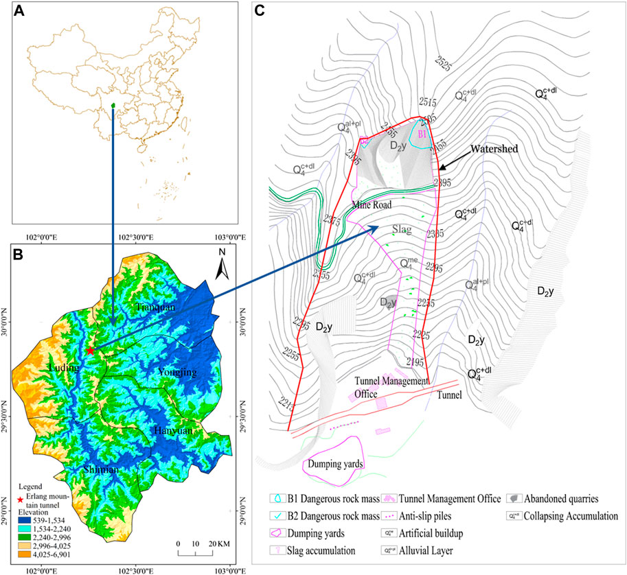
FIGURE 1. Distribution of debris flow basin on the back hillside of the Erlang Mountain Tunnel Management Office. (A) Location within China, (B) Location within Sichuan Province, (C) Location of the back hillside of Erlang Mountain Tunnel Management Office, and the surrounding environment distribution.

Slope debris distribution

There are many sources of debris on the hillside behind the Erlang Mountain Tunnel Management Office, including collapsed rocks from broken rock layers, alluvial deposits accumulated in valleys, slope deposits, abandoned earth, and rocks from mines. This provides favorable conditions for the generation of slope mudslides on the hillside behind the Erlang Mountain Tunnel Management Office. The constriction of the slope is approximately 140 m from the top of the slope. The topography of this section of the slope is wide at the top and narrow at the bottom, with a large area and large amount of debris that has accumulated (Figure 2A). Earthquakes have loosened deposits at this site, and a large amount of gravel and waste slag have been piled up in the gullies on the slope surface such that debris flow may likely occur on this slope. The deposition area is approximately 14,000 m², and the average deposition thickness is approximately 2–3 m. It is preliminarily estimated that the cumulative volume of gravel and waste slag in the mine is approximately 30,000 to 40,000 m³ (Figure 2B), and the gradient of the longitudinal slope of the trench bed in the waste slag field area is as large as 60%–100%. In addition, the gully on the slope is also relatively large, and it is generally between 25° and 35°.

FIGURE 2

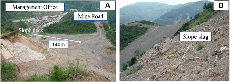
FIGURE 2. Survey on the back hillside of the west exit of the Erlang Mountain Tunnel Management Office. (A) Geometry of the slope behind the management office at the west entrance of Erlang Mountain Tunnel and the spatial relationship between the slope and management office. (B) Slag debris accumulated on the slope.

Inducing factors of slope debris flow

Based on the survey results, the average annual rainfall in the Erlang Mountain Tunnel area is 636.8 mm. However, this is a dry and hot valley area, and the rainfall is concentrated with a relatively high intensity an a maximum rate of 56 mm/10 min. The topographical structure on both sides of the back slope of the Erlang Mountain Management Office is a raised ridge wherein the middle terrain is low and easily collects water. The overall area is narrow, as shown in Figure 2A, with frequent rainstorms and concentrated rainfall. Rainfall starts at the top of the mountain and extends to the foot of the mountain to form a large flood peak. According to the Song et al. (2017) study, rainwater infiltration into the slope will soften the slope material and intensify the slope deformation. Strongly concentrated rainfall can cause rapid deformation of the slope surface providing a source of water for the occurrence of slope debris flow.

The hillside behind the Erlang Mountain Tunnel Management Office contains a large amount of mine waste slag (Q₄^me), as shown in Figure 3A, and the stability of this waste slag deteriorated because of earthquakes. The provenance volume is approximately 40,000 m³, which provides the main basis for slope debris flow. Years of rainfall has caused many gullies to form on the slope as the mine slope was eroded and became steeper. The height difference between the ditch bed and the top of the mountain also increased, making it easier for solid materials to enter the ditch bed. A constriction is also present on the slope, and a large amount of mine waste with extremely poor stability is present on the slope above the constriction. The relative height difference of the waste slag area is 180 m, and the slope is approximately 45°–58°, as shown in Figure 3B. Serious soil erosion has occurred on the slope, where sparse vegetation and exposed slope accretion is observed. Both topographic and geomorphological conditions have a direct impact on the occurrence of slope debris flow, which is easily formed when the slope is between 30° and 50° (Xu et al., 2005). The accumulated debris on the surface of these slopes can easily travel down the slope due to its own weight, and a slope debris flow may be formed in the presence of heavy rain. Because the flow rate of the debris flow remains unchanged, the terrain becomes narrower after passing through the constriction, thereby increasing the velocity, which increases the risk of slope debris flow.

FIGURE 3

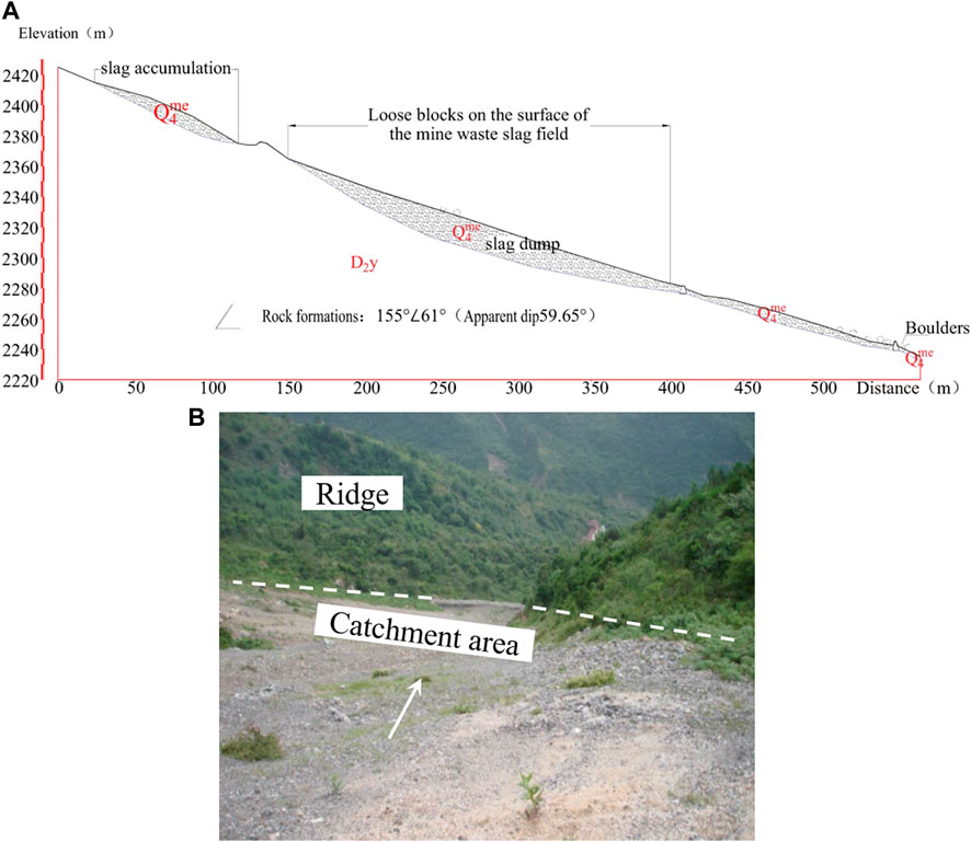
FIGURE 3. (A) Topographical graph of the hillside surface behind the west exit of the Erlang Mountain Tunnel Management Office and (B) slope surface catchment area.

Numerical simulation

Rheological and frictional models

RAMMS software is used to simulate the debris flow movement process, and data including the velocity, flow height, and impact momentum can be obtained during such simulations (Christen et al., 2010a). Hungr et al. (2005) indicated that uncertain conditions will affect the movement of debris flows, and it is therefore very important to select an appropriate rheological model when simulating continuous media. In the continuum model, the fluid is assumed to be an unstable and heterogeneous fluid, which is represented using the fluid height H and fluid velocity U (Deubelbeiss and Graf, 2013).

The velocity of this system is expressed as:

$U\left(x,y,t\right)={\left[U_x\left(x,y,t\right),U_y\left(x,y,t\right)\right]}^T(1)$

Here, $U_x$is the velocity in the x-direction, $U_y$is the velocity in the y-direction, and T is the transpose matrix of the average velocity.

The magnitude of the velocity is:

$\Vert U\Vert =\sqrt{U_x^2+U_y^2}(2)$

where $\Vert U\Vert$ is defined as the absolute average value of the velocity, which ensures that the velocity U is positive in the vector space.

The velocity direction is defined as:

$n_u=\frac{1}{\Vert U\Vert \left(U_x,U_y\right)}(3)$

where $n_u$ is a unit vector that is used to represent the direction of the fluid velocity.

The flow height is:

${\partial }_{t}H+{\partial }_x\left(H{U}_x\right)+{\partial }_y\left(H{U}_y\right)=Q\left(x,y,t\right)(4)$

where $Q\left(x,y,t\right)$ represents the accumulated flow such that, if Q=0, no deposition is present, and H represents the deposition height.

The Vollemy model simulates the friction of the fluid in the x and y directions on the slope (Slam. 1993). The friction is composed of the normal stress, the resistance of the velocity squared, and the dry Coulomb friction (µ) considering the viscous-turbulent friction coefficient (ζ). Eq. 5 is the friction resistance equation.

$S_f=\mu \rho g\cos \left(\varphi \right)+\frac{\rho g{\mu }^2}{\zeta }(5)$

Here, $S_f$ is the frictional resistance, $\rho$ is the fluid density, $g$ is the gravitational acceleration, and $\varphi$ is the slope.

The frictional resistance $S_f$ is composed of the friction forces in the x- and the y-directions, as follows:

$S_f=\left(S_{fx}+S_{fy}\right)(6)$

$S_{fx}=n{U}_x\left[\mu g_{z}H+\frac{g{\Vert U\Vert }^2}{\zeta }\right](7)$

$S_{fy}=n{U}_y\left[\mu g_{z}H+\frac{g{\Vert U\Vert }^2}{\zeta }\right](8)$

In Eq. 6, $S_{fx}$ represents the frictional resistance in the x-direction and $S_{fy}$ represents the frictional resistance in the y-direction.

In the x- and y-directions, the fluid height balance equations can be expressed as follows:

${\partial }_t\left(H{U}_x\right)+{\partial }_x\left(C_{x}H{U}_x^2+g_z{K}_{\alpha /P}\frac{H^2}{2}\right)+{\partial }_y\left(H{U}_x{U}_y\right)=S_{gx}-S_{fx}(9)$

${\partial }_t\left(H{U}_y\right)+{\partial }_y\left(C_{y}H{U}_y^2+g_z{K}_{\alpha /P}\frac{H^2}{2}\right)+{\partial }_y\left(H{U}_x{U}_y\right)=S_{gx}-S_{fy}(10)$

Here, $C_x$ and $C_y$ are the section coefficients, and $g_z$ is the gravitational acceleration in the vertical direction. In the Voellmy model, the contact relationship can be defined as a heterogeneous Molar-Coulomb relationship, where $K_{\alpha /p}$ is the earth pressure coefficient and is expressed as:

$K_{\alpha /p}={\tan }^2\left({45}^{\circ }\pm \frac{\varphi }{2}\right)(11)$

where $\varphi$ is the fluid internal friction angle.

Considering the above formulas, the Voellmy rheological formula can be obtained as:

$\frac{d\left(Uh\right)}{d_t}=\left(z•n\right)nh-k\left(\nabla h\right)h-\left[\mu \left(z•n\right)h+\frac{1}{\zeta }{U}^2\right]S(12)$

Here, the variables are measured considering the length L, velocity (gL/2), and time ((L/g)/2), respectively, to obtain a uniform Froude value. The gravity vector is z=(0, 0, -1).

Validation of the RAMMS software debris flow simulation method

The basic steps of debris flow simulations using RAMMS software are as follows. First, CAD software is used to draw contour lines for the study area through elevation points. Next, to import the topographic contour map into ArcGIS, the ArcToolbox is used to project the coordinate system into a Cartesian coordinates system that is compatible with RAMMS. The contour lines are then converted to the TIN irregular triangulation format, which is subsequently converted it to ASCII format. Finally, the ASCII terrain data are imported into RAMMS and the watershed range and provenance area data are exported for backup. RAMMS is then opened and the terrain model, provenance area, and watershed range are loaded into this program in turn. Thicknesses are then assigned to the provenance area according to the survey data.

In order to test the feasibility of the RAMMS for slope debris flow simulation, we consider the simulation conducted by Luo. (2020) based on the Flo-2d simulation of the Xiazhuang ditch debris flow involving field survey data. According to this study, the slope on both sides of the Xiazhuang ditch is 40°, the relative height difference in the watershed is 2,670 m, and the average slope of the channel bed is 262.4%. An earthquake caused the mudslide to occur with a final deposition area of 2.17×10⁴ m². The friction and turbulence coefficients simulated via RAMMS were set according to the recommended values in the user manual, and the remainder of the parameter settings were the same as those of Luo et al. or utilized the on-site survey data.

From Table 1, we can see the accumulation range and outflow volume of the debris flow in the Xiazhuang ditch under the condition of a 20-year rainfall period as determined by Flo-2d and RAMMS.

TABLE 1

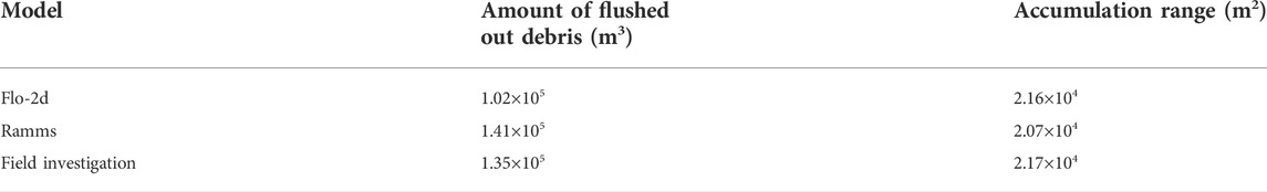
TABLE 1. Validation results for the RAMMS software debris flow simulation method.

The relative error is defined as:

$E=\frac{\left|A-B\right|}{B}\times 100\%(13)$

where E is the relative error, A is the comparison value, and B is the true value. It was found that the error between the RAMMS-simulated accumulation range and the field survey data was 4.61%, and the reliability of this simulation method was high. Compared to the data obtained onsite, the error of the debris flow was 4.44%, and the reliability was high. Compared with the Flo-2d simulation results, the relative error of the accumulation range was 4.17%, which indicates highly reliability, and the relative error associated with the amount of debris that was flushed out was relatively high.

Slope debris flow simulation parameter settings

We next studied the debris flows on the slope of the back hill of the Erlang Mountain Tunnel Management Office using RAMMS under various rainfall conditions. Two types of friction parameters, namely rainfall and provenance, are required for the simulation. The rainfall was obtained according to the “Hydrology Handbook of Sichuan Province”. In this study, the peak discharge values of torrential rain under four rainstorm frequencies of 1, 2, 5, and 10% for the Erlang Mountain Tunnel Management Office were utilized, and a debris flow hydrograph was designed according to the “Mountain Flood, Debris Flow, and Landslide Disaster and Prevention” guidelines.

The rainstorm peak flow is calculated via:

$Q_p=0.278\left(\frac{s}{{\tau }^n}-\mu \right)F(14)$

where Q_P is the peak flow of the rainstorm, where p is the rainstorm frequency; S is the designed rainstorm parameter; n is the rainstorm formula index representing the rainfall obtained from local data via the hydrology manual; τ is the confluence time, which is calculated according to the overall confluence; µ is the runoff coefficient, which represents the average infiltration capacity of the rainwater into the ground; and F is the confluence area, which is obtained based on the survey results.

The peak debris flow is calculated as:

$Q_{pc}=\left(1+{\varphi }_c\right)Q_p(15)$

Where φ_c is the sediment correction coefficient. In Eq. 14, φ_c is designated as 1.2 according to Wang (2004). The calculated debris flow is shown in Table 2.

TABLE 2

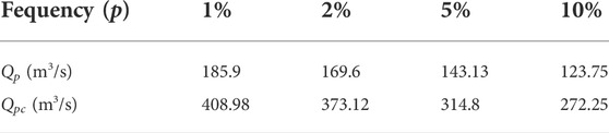
TABLE 2. Calculation value of rainstorm flow and debris flow.

The height and volume of the provenance were obtained from an on-site investigation, and the density of the provenance was set according to the debris flow in the Heping ditch of the Erlang Mountain Tunnel (Wang 2004). The simulation parameters include the model grid resolution, numerical calculation scheme, and simulation release method. The model grid resolution was set to 4 × 4 m, and the numerical calculation adopted a second-order precision. Hydrological curves were chosen for this simulation study to release debris flow. The friction and turbulence parameters were the same as those used for the comparative verification. The specific parameters are listed in Table 3.

TABLE 3

TABLE 3. Slope debris flow simulation parameters.

Results and discussion

Influence of friction coefficient on the movement process of slope debris flow of Erlang Mountain Tunnel Management Office

Topographical changes can occur many years after the occurrence of a debris flow (Schneider et al., 2014). Vegetation causes significant reduction in the debris flow velocity (Christen et al., 2017). Moreover, a smaller slope corresponds to a smaller friction force related to the loose deposits and a greater influence on the maximum accumulation thickness and maximum velocity of the debris flow (Lee et al., 2015). The Voellmy model considers changes in the turbulence coefficient ζ and dry Coulomb friction coefficient μ to account for topographical conditions (Christen et al., 2010b). The turbulence coefficient ζ has a significant influence on high-speed debris flows. Pirulli and Sorbino (2008) indicated that the ζ value should be in the range of 100–1,000 m/s², and Christen et al. (2010a) found that the extereme ζ value is 3,000 m\s². When the debris flow is slow, it is significantly affected by dry Coulomb friction μ. The value of μ generally between 0.05 and 0.4. When it exceeds 0.4, the simulation results become highly inaccurate (Deubelbeiss and Graf 2013). To determine the effect of landform on the accumulation range of the debris flow on the back hillside of the Erlang Mountain Tunnel Management Office, the variation of the friction coefficient was investigated (Figure 4).

FIGURE 4

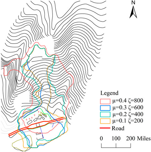
FIGURE 4. Influence of various friction coefficients on the accumulation range observed during debris flow.

As shown in Figure 4, the overall debris flow process was similar for all friction coefficients. However, as the frictional resistance coefficient increased, the debris flow was prevented from moving downward, which increases the time required for the debris flow to flow down the slope and increases the deposition height on the slope. This results in the lateral expansion of the debris flow range. When the dry Coulomb friction value μ increased from 0.3 to 0.4, the debris no longer flowed from the slope into the channel and instead began to spread out along the slope. Moreover, the accumulation area at the management site was significantly reduced, and the flow velocity decreased. Considering the effect of friction on debris flow, the damage resulting from debris flow can be reduced by altering the landscape. Shelter forests can be planted on exposed slopes to increase the frictional force opposing debris flow and reduce the occurrence of runoff. It is also possible to dispose of loose deposits located on the slopes behind the Erlang Mountain Tunnel Management Office to reduce the stacking height and slope incline while increasing the friction, thereby reducing debris flow hazards.

Simulation of debris flow on the slope surface under the 20-year rainfall condition

The deposition height and flow velocity are two important criteria for evaluating debris flow disasters. They can reflect the movement characteristics and degree of damage resulting from debris flow. The flow velocity determines the ability of the debris flow to cause damage via impact, while the deposition height reflects its ability to cause damage via burying. The most recent debris flow near the west entrance of the Erlang Mountain Tunnel occurred in 1997, and therefore the condition of rainfall occurring once in 20 years was selected to numerically investigate the debris flow on the slope of the Erlang Mountain Tunnel Management Office. The variations in the flow velocity (Figure 5) and deposition height (Figure 7) of the debris flow on the slope for different movement time-histories in this area were obtained.

FIGURE 5

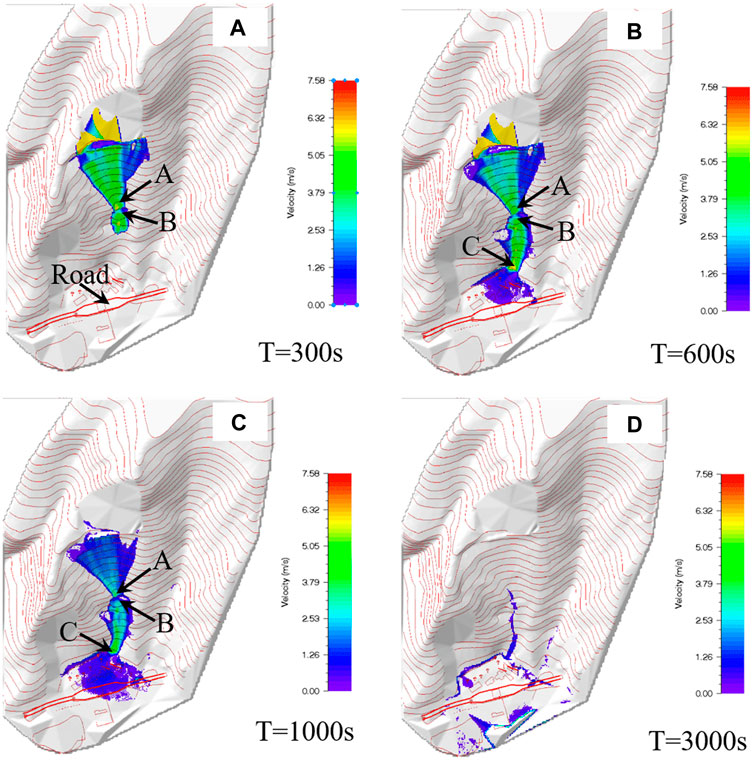
FIGURE 5. Variation of the flow velocity of debris on the slope surface under the condition of exteme rainfall once every 20 years at (A) t=150 s, (B) t=600 s, (C) t=1,000 s, and (D) t=3,000 s.

The flow velocity of debris flow is an important parameter for determining its ability to cause damage, and it is very important to study the change in flow velocity during debris flow (Cui and Zou. 2016). As shown in Figure 5, under the condition of extreme rainfall once every 20 years, the flow of debris on the hillside behind the Erlang Mountain Tunnel Management Office can be divided into four processes: the initial slope acceleration of the debris flow, the deceleration of the flow that contacts the mountain, the re-acceleration of the debris through the constriction, and the slowly spread of the debris.

When the debris flow starts to move during the early stage, it crosses the mining road and reaches the upper slope of the constriction area. The initial flow velocity is proportional to time, and the speed increases, as shown by point A in Figure 5A. After the debris has flowed for 150 s, the speed at point A is 5.99 m/s. This is because the gravitational potential energy of the debris flow is converted into kinetic energy, the instantaneous velocity increases, and the topography of the initial slope cannot produce a large resistance to the flow. This represents the acceleration stage along the initial slope of the debris flow. The velocity of the debris flow decreases for a short period of time after passing through the constriction, as shown by point B in Figure 5A. When the debris flow has flowed for 150 s, the velocity of point B is 4.05 m/s. From the topographic analysis, this velocity results from the narrow terrain at the constriction and the topographic deflection effect on the upper slope, which cause the debris flow to impact the mountain, thereby reducing its speed. This represents the deceleration section of the debris flow as it impacts the mountain. After the debris flow has passed through the constriction, it enters the gully and exhibits a rapid increase in velocity, as shown by points B and C in Figure 5B. At this time, the speed of point B is 3.47 m/s and that of point C is 5.79 m/s. This occurs because the instantaneous velocity of the debris flow increases as the slope narrows; in the case of years of heavy rain, the gully under the slope is eroded, the slope becomes steeper, and the gully length is increased by approximately 150 m (Figure 2A). The larger slope, slope length, and topographic indentation are the key factors that result in the re-acceleration of the debris flow after entering the gully, and the entire process of the debris flow from the beginning to when it flows into the accumulation area occurs over approximately 4 min. After the debris flow enterseds the management area, the terrain suddenly changes from steep to flat, the flow velocity decreases sharply, and siltation occurrs until the velocity reaches 0. These processes occur because terrain deflection has a significant effect on the gravitational potential energy of the debris flow, which causes an instantaneous reduction in the debris flow velocity and generates a large impact force, causing a large amount of damage to the platform of the Erlang Mountain Tunnel Management Office.

To better study the influence of the slope constriction on the dynamic process of debris flow, two points (points A and C in Figure 5B) are selected upstream and downstream of the slope constriction for analysis, and the flow velocity and rate are obtained. The simulation results are shown in Figure 6. The velocity at point A is 3.99 m/s, the discharge is 148.40 m³/s, the velocity at point C is 5.79 m/s, and the discharge is 173.51 m³/s. Apparently, during the downstream movement of the debris flow, the flow velocity and discharge along the way show a significant amplification effect; the flow velocity is amplified by 31.1%, and the discharge by 14.5%. Generally speaking, in valley debris flows, the amplification effect is mainly related to channel blockage, slag dam failure, and landslide provenance recharge (Liu et al., 2021). Song et al. (2018) believes that slope, elevation, and slope micro-topography have an impact on the slope magnification effect. However, in this study, the gullies were not blocked or supplied by provenance and the slope of the surface did not change significantly. After excluding the above factors, it was concluded that slope constriction is also a key factor in the amplification of debris flow velocity and flow. For the prevention and control of such slopes debris flow, it is necessary to adopt blocking works in the middle or upstream of the slope constriction or increase the terrain friction to minimize the influence of the slope indentation on the flow velocity and flow amplification effect and reduce the degree of debris flow disaster.

FIGURE 6

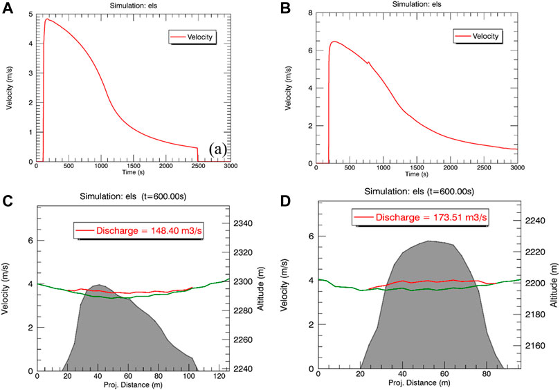
FIGURE 6. Comparison of velocity and flow at point A and point C of the debris flow on the slope surface at 600 s. Flow velocity at 600 s at point (A) A and (B) (C). Discharge of (C) A section and (D) C section.

During the flow of debris, the maximum accumulation thickness may result in a building being buried, overturned, or collapsed. From it can be seen that the debris flow will accumulates in a short period of time owing to the obstruction of the mining road. As shown in Figure 7A, the stacking height of point A is approximately 3.87 m. The debris then continues to flow downward into a broad slope without forming a large accumulation. The second accumulation of debris occurs at the constriction point located 300 m from the release area, as shown by point B in Figure 7A. The simulation showed that the deposition height of point B is 3.12 m after the debris has flowed for 150 s. Because this is the connection point between the narrowing of the slope and the turn of the gully below, the mouth of the gully is narrow, and the debris flow rate on the slope during the initial stage of release is relatively large. A large amount of debris accumulates at this location, causing a blockage during the flow process, and the deposition height increases rapidly. When the debris flows through the gullies below the narrow slope passage, no deposition occurs. The third debris flow accumulation occurs at the tunnel management point located 550–600 m from the debris flow initiation area, as shown by point C in Figure 7B. The accumulation of the debris flow produces a faucet, and the deposition height at point C is 8.13 m. This accumulation occurs due to the sudden decrese in the terrain slope at the Erlang Mountain Tunnel Management Office, which hinders the movement of the debris flow. When the debris flow moves toward a larger slope, the resistance of the front section of this flow is small with a fast velocity, while the velocity of the rear section is slow owing to the obstruction of the front section of the debris flow. When the terrain suddenly changes to a small slope, the resistance increases and the movement speed decreases, causing the accumulated debris to impact and ascend the mountain, thereby producing accumulation faucets. After the debris flow has reached the management platform, a fan-shaped deposition begins to form, as shown in Figure 7D. After the debris flow has reached the platform of the management office, a fan-shaped deposition begins to form, as shown in Figure 7D. After flowing through the mining road, the debris flow slowly spreads downward owing to the obstruction of the mountain, and a small accumulation of debris occurs on the mountain, as shown by point D in Figure 7D. Here, the deposition height is 3.87 m, the overall average deposition height is approximately 0.835 m, the deposition area is approximately 129,500 m², and the total accumulation volume is 132562.14 m³.

FIGURE 7

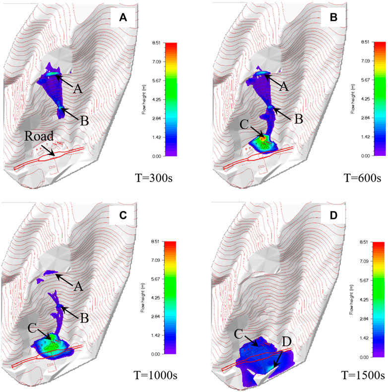
FIGURE 7. Variation of the deposition height of the debris flow on the slope surface under the condition of extreme rainfall once every 20 years at (A) t=150 s, (B) t=600 s, (C) t=1,000 s, and (D) t=3,000 s.

Risk assessment

Debris flow risk zoning is mainly based on the flow velocity and height of the debris. Hubl and Steinwendtner (2001) used Flo-2d software to simulate two debris flows in Austria and differentiated the two flows based on their velocity and height. Tang et al. (1994) indicated that the accumulation area can be divided into four classifications indicating their danger according to the flow velocity and height. These parameters can be determined using dynamic software simulations, and the risk assessment of the concerned area can be conducted (Hu and Wei 2005).

Based on the Voellmy model in the RAMMS software, this study numerically simulated the debris flow on the slope of Erlang Mountain and predicted the flow velocity, depth, and accumulation under the condition of a heavy rainfall occurring once every 20 years. We may then evaluate the risk of damage associated with this debris flow based on its velocity or depth according to the method provided by Tang et al. (1994), as shown in Table 4.

TABLE 4

TABLE 4. Hazardous area classifications.

The maximum deposition height of each position in the debris flow process was obtained via simulation, and ArcGIS was used to convert the deposition height and obtain a hazard zoning map of the study area (Figure 8). The different colors in the figure correspond to the different levels of danger caused by the debris flow. This map shows that the extremely high-risk area in the debris flow basin accounts for 9.3% of the total area, the high-risk area accounts for 24.6% of the total area, the medium-risk area accounts for 15.6% of the total area, and the low-risk area accounts for 50.4% of the total area. The results showed that the main slope of the debris flow on the backside of the Erlang Mountain Tunnel Management Office was comparatively less dangerous than the national highway 318 area, while the Management Office platform area was extremely dangerous. After the slope debris flows, the national highway 318 will be blocked, which will seriously affect traffic and safety of the platform management personnel. Therefore, it is necessary to frequently monitor rainfall during heavy rainstorms along the rear mountain of the Erlang Mountain Tunnel Management Office. Precautions should also be taken to prevent debris flow disasters during extreme rainstorm conditions that threaten the productivity and safety of personnel in the traffic and management office.

FIGURE 8

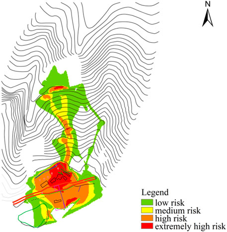
FIGURE 8. Predicted zoning map of the debris flow risk on the Erlang Mountain slope under the condition of a heavy rainfall once every 20 years.

Conclusion

Through an on-site investigation of the slope behind the west entrance of the Erlang Mountain Tunnel Management Office, the causes of debris flow were analyzed. In this paper, RAMMS software is used to provide a new method for predicting the dynamic process of slope debris flow. The dynamic process of debris flow on the slope surface under the condition of a heavy rainfall once every 20 years was simulated, and a risk assessment of the study area was based on the debris flow deposition height and velocity. The following conclusions may be drawn.

(1) The relative elevation difference of the mountain slope behind the Erlang Mountain Tunnel Management Office is greater than 600 m and the slope varies significantly. It is a typical slope debris flow. The main reason is that the study area has easy water catchment area and short-term heavy rainfall. Moreover, earthquake action and mining provide abundant material sources for the formation of debris flow.

(2) The dynamic process of debris flow on the backside of the Erlang Mountain Tunnel Management Office can be divided into four stages. The simulation results show that the back hill of Erlang Mountain Tunnel Management Office possesses characteristics of the slope constriction, which will increase the flow rate by 31.1% and discharge by 14.5% and cause severe harm to the management office. The simulation results show that the base friction limit μ of the slope debris flow changes from downstream to lateral diffusion is in the range of 0.3–0.4. The simulation results are helpful for understanding the degree of danger and the scope of disaster after the occurrence of debris flow.

(3) Debris flow hazard is divided into four levels according to flow velocity and accumulation height. Combined with the simulation results, a hazard prediction map for the 20-year return period of the debris flow on the backside of the Erlang Mountain Tunnel Management Office was drawn, and the extremely high risk area accounted for 9.3%. The risk prediction map has a reference value for the prediction and prevention of debris flow disasters in the region.

Because there are too many influencing factors in the process of debris flow movement, numerical simulation usually does not fully consider the practical factors. This study did not consider the influence of different rainfall return periods on the dynamic process of debris flow on the slope, which will be improved in future work.

Data availability statement

The original contributions presented in the study are included in the article/supplementarymaterial, further inquiries can be directed to the corresponding author.

Author contributions

Methodology, HW; Resources, HW; Funding, HW; Test, LD, DP, JY, TY, and DF; Data sorting, LD; Visualization, LD, TY, and DF; First draft preparation, HW and LD; Write comments and edit, HW, LD, JY, DP, TY, and DF; supervise, HW; Project administration, TY.

Funding

All authors thank the youth project of Henan Natural Science Foundation (Grant No. 212300410125), the China Postdoctoral Science Foundation General Project (Grant No. 2020M672202), the key projects of universities in Henan Province (Grant No. 20A570002), and the project supported by the open research fund of the Engineering Research Center for Embankment Safety and Disease Control of Ministry of Water Resources (No. LSDP202202) for supporting this study.

Acknowledgments

All authors thank the constructive review of the reviewer and editor for the early version of the manuscript.

Conflict of interest

The authors declare that the research was conducted in the absence of any commercial or financial relationships that could be construed as a potential conflict of interest.

Publisher’s note

All claims expressed in this article are solely those of the authors and do not necessarily represent those of their affiliated organizations, or those of the publisher, the editors and the reviewers. Any product that may be evaluated in this article, or claim that may be made by its manufacturer, is not guaranteed or endorsed by the publisher.

References

Bertolo, P., and Gerald, F. (2005). Calibration of numerical models for small debris flows in Yosemite Valley, California, USA. Nat. Hazards Earth Syst. Sci. 5, 993–1001. doi:10.5194/nhess-5-993-2005

CrossRef Full Text | Google Scholar

Catherine, B., McArdell, B. W., and Lauber, G. (2012). Debris flow simulation at illgraben, Switzerland, using 2d numerical model RAMMS debris-flow modeling application in practice. Bern, Switzerland: Environmental Science Elsevier.

Google Scholar

Christen, M., Bartelt, P., and Kowalski, J. (2010a). Back calculation of the in den Arelen avalanche with RAMMS: Interpretation of model results. Ann. Glaciol. 51 (54), 161–168. doi:10.3189/172756410791386553

CrossRef Full Text | Google Scholar

Christen, M., Kowalski, J., and Bartelt, P. (2010b). Ramms: Numerical simulation of dense snow avalanches in three-dimensional terrain. Cold Reg. Sci. Technol. 63 (1-2), 1–14. doi:10.1016/j.coldregions.2010.04.005

CrossRef Full Text | Google Scholar

Claudia, V. (2019). “Possibilities and limitations for the back analysis of an event in mountain areas on the coast of São Paulo State, Brazil using RAMMS numerical simulation,” in Contained in: Proceedings of the seventh international conference on debris-flow hazards mitigation (Golden, Colorado, USA. doi:10.25676/11124/173189

CrossRef Full Text | Google Scholar

Cui, P., and Zou, Q. (2016). Theory and method of risk assessment and risk management of debris flows and flash floods. Prog. Geogr. 35 (02), 137–147. (In Chinese). doi:10.18306/dlkxjz.2016.02.001

CrossRef Full Text | Google Scholar

Deubelbeiss, Y., and Graf, C. (2013). Two different starting conditions in numerical debris flow models–Case study at Dorfbach, Randa (Valais, Switzerland),” in Mattertal–ein Tal in Bewegung Editor C. GRAF. Publikation zur Jahrestagung der Schweizerischen Geomorphologischen Gesellschaf 29, 125.

Google Scholar

Egashira, S., Honda, N., and Itoh, T. (2001). Experimental study on the entrainment of bed material into debris flow. Phys. Chem. Earth, Part C Sol. Terr. Planet. Sci. 26 (9), 645–650. doi:10.1016/S1464-1917(01)00062-9

CrossRef Full Text | Google Scholar

Frey, H., Huggel, C., Bühler, Y., Buis, D., Burga, M. D., Choquevilca, W., et al. (2016). A robust debris-flow and GLOF risk management strategy for a data-scarce catchment in Santa Teresa, Peru. Landslides 13 (6), 1493–1507. doi:10.1007/s10346-015-0669-z

CrossRef Full Text | Google Scholar

Hu, K., and Wei, F. (2005). Debris flow hazard zoning method based on numerical simulation[J]. J. Nat. Disasters 14 (1), 10 (In Chinese). doi:10.3969/j.issn.1004-4574.2005.01.002

CrossRef Full Text | Google Scholar

Huang, R. Q., and Li, W. L. (2009). Analysis on the number and density of landslides triggered by the 2008 Wenchuan earthquake, China. J. Geol. Hazards Environ. Preserv. 20, 1 (In Chinese). doi:10.3969/j.issn.1006-4362.2009.03.001

CrossRef Full Text | Google Scholar

Hübl, J., and Steinwendtner, H. (2001). Two-dimensional simulation of two viscous debris flows in Austria. Phys. Chem. Earth, Part C Sol. Terr. Planet. Sci. 26 (9), 639–644. doi:10.1016/S1464-1917(01)00061-7

CrossRef Full Text | Google Scholar

Hungr, O. (1995). A model for the runout analysis of rapid flow slides, debris flows, and avalanches. Can. Geotech. J. 32 (4), 610–623. doi:10.1139/t95-063

CrossRef Full Text | Google Scholar

Hungr, O., Corominas, J., and Eberhardt, E. (2005). Estimating landslide motion mechanism, travel distance and velocity. Vancouver: Landslide risk management, CRC Press. [M]CRC Press 109-138. doi:10.1201/9781439833711-7

CrossRef Full Text | Google Scholar

Hungr, O. (2008). Simplified models of spreading flow of dry granular material. Can. Geotech. J. 45 (8), 1156–1168. doi:10.1139/T08-059

CrossRef Full Text | Google Scholar

Hutter, K., and Nohguchi, Y. (1990). Similarity solutions for a Voellmy model of snow avalanches with finite mass. Acta Mech. 82 (1), 99–127. doi:10.1007/BF01173741

CrossRef Full Text | Google Scholar

Jeremy, D. B., Stanford, G., Hiroshi, T., and Fumihiko, I. (2015). On the need for larger Manning's roughness coefficients in depth-integrated tsunami inundation models. Coast. Eng. J. 57 (2), 1550005-1–1550005-13155000513. doi:10.1142/S0578563415500059

CrossRef Full Text | Google Scholar

Lang, T. E., Dawson, K. L., and Martinelli, M. (1979). Application of numerical transient fluid dynamics to snow avalanche flow. Part I. Development of computer program avalnch. J. Glaciol. 22 (86), 107–115. doi:10.3189/S0022143000014088

CrossRef Full Text | Google Scholar

Lee, J. S., Song, C. G., Kim, H. T., and Lee, S. O. (2015). Effect of land slope on propagation due to debris flow behavior. J. Korean Soc. Saf. 30 (3), 52–58. doi:10.14346/JKOSOS.2015.30.3.52

CrossRef Full Text | Google Scholar

Li, Y., Wang, Z., Shi, W., and Wang, X. (2010). Slope debris flows in the Wenchuan Earthquake area. J. Mt. Sci. 7 (3), 226–233. doi:10.1007/s11629-010-2014-2

CrossRef Full Text | Google Scholar

Liu, B., Hu, X., Ma, G., He, K., Wu, M., and Liu, D. (2021). Back calculation and hazard prediction of a debris flow in Wenchuan meizoseismal area, China. Bull. Eng. Geol. Environ. 80, 3457–3474. doi:10.1007/s10064-021-02127-3

CrossRef Full Text | Google Scholar

Liu, K. F., and Mei, C. C. (1989). Slow spreading of a sheet of Bingham fluid on an inclined plane. J. Fluid Mech. 207, 505–529. doi:10.1017/S0022112089002685

CrossRef Full Text | Google Scholar

Liu, W., and He, S. (2018). Dynamic simulation of a mountain disaster chain: Landslides, barrier lakes, and outburst floods. Nat. Hazards (Dordr). 90 (2), 757–775. doi:10.1007/s11069-017-3073-2

CrossRef Full Text | Google Scholar

Luo, B. (2020). Analysis on the origin of "8·20" debris flow in xiazhuang ditch, wenchuan county, sichuan province and prediction of the scope of river blockage [J]. Bull. Soil Water Conservation 40 (06), 193–199. doi:10.13961/j.cnki.stbctb.2020.06.028

CrossRef Full Text | Google Scholar

Manzella, I., and Labiouse, V. (2008). Qualitative analysis of rock avalanches propagation by means of physical modelling of non-constrained gravel flows. Rock Mech. Rock Eng. 41 (1), 133–151. doi:10.1007/s00603-007-0134-y

CrossRef Full Text | Google Scholar

Medina, V., Hürlimann, M., and Bateman, A. (2008). Application of FLATModel, a 2D finite volume code, to debris flows in the northeastern part of the Iberian Peninsula. Landslides 5, 127–142. doi:10.1007/s10346-007-0102-3

CrossRef Full Text | Google Scholar

O'Brien, J. S., Julien, P. Y., and Fullerton, W. T. (1993). Two-dimensional water flood and mudflow simulation[J]. J. Hydrol. Eng. 119119 (2), 2442–3261. doi:10.1061/(ASCE)0733-9429

CrossRef Full Text | Google Scholar

Pirulli, M., and Sorbino, G. (2008). Assessing potential debris flow runout: A comparison of two simulation models. Nat. Hazards Earth Syst. Sci. 8 (4), 961–971. doi:10.5194/nhess-8-961-2008

CrossRef Full Text | Google Scholar

Salm, B. (1993). Flow, flow transition and runout distances of flowing avalanches. Ann. Glaciol. 18, 221–226. doi:10.3189/S0260305500011551

CrossRef Full Text | Google Scholar

Schamber, D. R., and MacArthur, R. C. (1985). One-dimensional model for mud flows[M]. Davis, CA: US Army Corps of Engineers, Hydrologic Engineering Center.

Google Scholar

Schneider, D., Huggel, C., Cochachin, A., Guillen, S., and Garcia, J. (2014). Mapping hazards from glacier lake outburst floods based on modelling of process cascades at Lake 513, Carhuaz, Peru. Adv. Geosci. 35, 145–155. doi:10.5194/adgeo-35-145-2014

CrossRef Full Text | Google Scholar

Song, D., Che, A., Chen, Z., and Ge, X. (2018). Seismic stability of a rock slope with discontinuities under rapid water drawdown and earthquakes in large-scale shaking table tests. Eng. Geol. 245, 153–168. doi:10.1016/j.enggeo.2018.08.011

CrossRef Full Text | Google Scholar

Song, D., Che, A., Zhu, R. Ge X., and Ge, X. (2017). Dynamic response characteristics of a rock slope with discontinuous joints under the combined action of earthquakes and rapid water drawdown. Landslides 15, 1109–1125. doi:10.1007/s10346-017-0932-6

CrossRef Full Text | Google Scholar

Song, D., Liu, X., Huang, J., and Zhang, J. (2021c2021). Energy-based analysis of seismic failure mechanism of a rock slope with discontinuities using Hilbert-huang transform and marginal Spectrum in the time-frequency domain. Landslides 18, 105–123. doi:10.1007/s10346-020-01491-7

CrossRef Full Text | Google Scholar

Song, D., Liu, X., Huang, J., Zhang, Y., Zhang, J., and Nkwenti, B. (2021a). Seismic cumulative failure effects on a reservoir bank slope with a complex geological structure considering plastic deformation characteristics using shaking table tests. Eng. Geol. 2021 (3), 106085. doi:10.1016/j.enggeo.2021.106085

CrossRef Full Text | Google Scholar

Song, D., Liu, X., Li, B., Zhang, J., and Vocan, J. (2021b2021). Assessing the influence of a rapid water drawdown on the seismic response characteristics of a reservoir rock slope using time-frequency analysis. Acta Geotech. 16, 1281–1302. doi:10.1007/s11440-020-01094-5

CrossRef Full Text | Google Scholar

Tang, J., Chen, L., and Wang, G. (1994). Numerical simulation research on zonal assessment of risk degree of debris flow accumulation fan[J]. J. Catastrophology (04), 7–13. (In Chinese) http://dx.chinadoi.cn/cnki:sun:zhxu.0.1994-04-001.

Google Scholar

Wang, F., Wu, Y. H., Yang, H., Tanida, Y., and Kamei, A. (2015). Preliminary investigation of the 20 August 2014 debris flows triggered by a severe rainstorm in Hiroshima City, Japan. Geoenvironmental Disasters 2 (1), 17–16. doi:10.1186/s40677-015-0025-6

CrossRef Full Text | Google Scholar

Wang, X. Q. (2004). Research and control design of debris flow characteristics in Erlangshan Tunnel of Sichuan-Tibet Highway[J]. Adv. Earth Sci. (S1), 7. (In Chinese) http://dx.chinadoi.cn/cnki:sun:dxjz.0.2004-s1-080.

Google Scholar

Worni, R., Huggel, C., and Stoffel, M. (2013). Glacial lakes in the Indian Himalayas — from an area-wide glacial lake inventory to on-site and modeling based risk assessment of critical glacial lakes. Sci. Total Environ. 468, S71–S84. doi:10.1016/j.scitotenv.2012.11.043

PubMed Abstract | CrossRef Full Text | Google Scholar

Worni, R., Stoffel, M., Huggel, C., Volz, C., Casteller, A., and Luckman, B. (2012). Analysis and dynamic modeling of a moraine failure and glacier lake outburst flood at Ventisquero Negro, Patagonian Andes (Argentina). J. Hydrol. X. 444, 134–145. doi:10.1016/j.jhydrol.2012.04.013

CrossRef Full Text | Google Scholar

Yongshuang, Z., Shuwen, D., Chuntang, H., Changbao, G., Xin, Y., Bin, L., et al. (2013). Geohazards induced by the lushan Ms7.0 earthquake in sichuan Province, southwest China: Typical examples, types and distributional characteristics. Acta Geol. Sin-Engl 87 (3), 646–657. doi:10.1111/1755-6724.12076

CrossRef Full Text | Google Scholar

Zimmermann, F., McArdell, B., Rickli, C., et al. (2018). Does cohesion improve the accuracy of runout of hillslope debris flows? A systematic comparison using well-documented events in Switzerland. Vienna, Austria: EGU General Assembly Conference Abstracts.

Google Scholar