 Gang Feng
 Hua-Hui Zeng
 Xing-Rong Xu1
 Gen-Yang Tang
95% of researchers rate our articles as excellent or good
Learn more about the work of our research integrity team to safeguard the quality of each article we publish.
Find out more
ORIGINAL RESEARCH article
Front. Earth Sci. , 11 January 2023
Sec. Environmental Informatics and Remote Sensing
Volume 10 - 2022 | https://doi.org/10.3389/feart.2022.1025635
This article is part of the Research Topic Advances and Applications of Artificial Intelligence in Geoscience and Remote Sensing View all 14 articles
Shear wave velocity plays an important role in both reservoir prediction and pre-stack inversion. However, the current deep learning-based shear wave velocity prediction methods have certain limitations, including lack of training dataset, poor model generalization, and poor physical interpretability. In this study, the theoretical rock physics models are introduced into the construction of the labeled dataset for deep learning algorithms, and a forward simulation of the theoretical rock physics models is utilized to supplement the dataset that incorporates geological and geophysical knowledge. This markedly increases the physical interpretability of the deep learning algorithm. Theoretical rock physics models for two different types of reservoirs, i.e., conventional sandstone and tight sandstone reservoirs, are first established. Then, a full-sample labeled dataset is constructed using these two types of theoretical rock physics models to traverse the elasticity parameter space of the two types of reservoirs through random variation and combination of parameters in the theoretical models. Finally, based on the constructed full-sample labeled dataset, four parameters (P-wave velocity, clay content, porosity, and density) that are highly correlated with the shear wave velocity are selected and combined with a deep neural network to build a deep shear wave velocity prediction network with good generalization and robustness, which can be directly applied to field data. The errors between the predicted shear wave velocity using the deep neural network and the measured shear wave velocity data in the laboratory and the logging data in three real field work areas are less than 5%, which are much smaller than the errors predicted by both Han’s and Castagna’s empirical formula. Furthermore, the prediction accuracy and generalization performance are better than those of these two common empirical formulas. The forward simulation based on theoretical models supplements the training dataset and provides high-quality labels for machine learning. This can considerably improve the interpretability and generalization of models in real applications of a machine learning algorithm.
Shear wave (S-wave) velocity plays an important role in reservoir prediction (Du, 2014). S-wave velocity data are required for pre-stack inversion and pre-stack attribute analysis. However, in real field work areas, especially in old wells, the high cost of acquiring shear wave velocity data leads to lack of S-wave velocity data (Bagheripour et al., 2015). Therefore, predicting the S-wave velocity in wells where these values has not been measured is essential. The conventional S-wave velocity prediction methods can be divided into three categories, empirical formula method, theoretical rock physics model method and machine learning prediction method.
The empirical formula method utilizes the existing logging data from the target area to statistically analyze the relationship between these data and the S-wave velocity. The formula is generally obtained by fitting data point pairs based on some kind of mathematical expression. There is no need to have a complete theoretical derivation process, and this method is only applicable to specific geological environments (Castagna et al., 1985; Han et al., 1986; Eberhart-Phillips et al., 1989; Ameen et al., 2009). The rock physics model prediction method is to establish the relationship between elastic parameters and reservoir parameters based on theoretical models. Therefore, the S-wave velocity prediction is often more accurate than the empirical formula (Gassmann, 1951; Biot, 1956; Xu and White, 1995, 1996; Xu and Payne, 2009; Sun et al., 2012). Theoretically, the rock physical model is not specifically limited to a particular region, but there is a lot of noise in the real field data, and the predicted results have great uncertainty. In addition, the application of the rock physics model to predict S-wave velocity needs to consider the influence of skeleton composition, fluid distribution and pore shape, which make the application of the rock physics model to predict shear wave velocity difficult since there parameters are not easily accessible.
Neural networks have great advantages in dealing with nonlinear problems, and S-wave velocity prediction is a typical nonlinear problem. In recent years, S-wave velocity prediction using well log data and back-propagation neural network (BPNN) has been widely applied in practical field areas (Eskandari et al., 2004; Alimoradi et al., 2011; Maleki et al., 2014). Each hidden layer of the recurrent neural networks (RNNs) has a feedback to a previous layer, and the subsequent behavior can be shaped by the response of the previous layer. Thus, RNNs are well suited for processing sequential data, and since logging data are connected in-depth, RNNs and their variants long short-term memory (LSTM) networks and gated recurrent units (GRU) networks have been introduced into the S-wave velocity prediction (Mehrgini et al., 2017; Zhang et al., 2020) and other rock parameters (Yuan et al., 2022). Moreover, convolutional neural networks (CNNs) have tremendous advantages in feature extraction, thus the CNNs were widely developed and applied in many research fields (Yuan et al., 2018; Hu et al., 2020; Hu et al., 2021), and a combination of RNNs and CNNs for S-wave velocity prediction has been proposed recently (Wang et al., 2022; Zhang et al., 2022). However, the neural network-based S-wave velocity prediction method has poor generalization and limited labels for establishing S-wave velocity prediction networks, which brings many difficulties to real applications.
To overcome these limitations, we combine theoretical rock physics models and deep neural networks (DNNs) for S-wave velocity prediction. Synthetic datasets can be used when building labeled datasets, if the synthetic datasets are sufficiently complicated, that is, if the most important factors are considered when generating the datasets, the trained network may be able to process realistic datasets directly (Wu et al., 2019; Yu and Ma, 2021; Gao et al., 2022). Therefore, a rich and complete labeled dataset is first constructed using the theoretical rock physics models, and then a deep S-wave velocity prediction network is established using the DNN and the data, such as the P-wave velocity and porosity in the full-sample labeled dataset. Instead of using the data of a certain area to train the neural network, the data generated by the theoretical rock physics models are used for the training, and then the established network is directly applied to the real target work area for S-wave velocity prediction.
The rock physics model can link the elastic parameters to physical parameters, fluid and lithology (Guo et al., 2022), and specific theoretical rock physic model needs to be established for different types of reservoirs due to different composition, texture and pore microstructure of the reservoir rocks.
The porosity and permeability of the conventional sandstone are quite high with relatively simple pore geometry, so the conventional sandstone reservoir is high-quality reservoir. In this study, the Voigt-Ruess-Hill (VRH; Hill, 1952) model is used to calculate the moduli of the rock matrix, and then the Kuster-Toksöz model (Kuster and Toksőz, 1974) is utilized to add stiff and compliant pores to the rock matrix to calculate the moduli of the dry skeleton, which are expressed as follows:
where
Then the Wood model is utilized to calculate the bulk moduli of the mixed fluid, and finally, the Gassmann equation (Gassmann, 1951) is used to calculate the saturated rock moduli.
where
For tight sandstone reservoirs, the heterogeneity, microscopic pore structure and pore fluid distribution of rocks are quite complex (Guo et al., 2021). When saturated with different fluids, the fluid flow caused by wave propagation makes the overall elastic responses of rocks more complex. For tight sandstone reservoirs, firstly, the moduli of the rock skeleton are also calculated using the VRH model and the Kuster-Toksöz model, and then the squirt flow effect is considered to account for the velocity dispersion and attenuation (White, 1975; Dvorkin et al., 1995). A simple squirt flow model (Gurevich et al., 2010) can be used to characterize the wave-induced flow effects occurring at microscopic scales in tight sandstones. The idea of a simple squirt flow model is to modify the dry skeleton of the rock as if the compliant pores are saturated with fluid and the stiff pores remain dry, which are expressed as follows:
where
After obtaining the modified dry skeleton moduli, the saturated rock elastic moduli are calculated by the Gassmann fluid substitution equations (Han et al., 2021) as follows:
where
According to the established theoretical rock physics models, the bulk moduli, the shear moduli can be obtained, and the P-wave velocity and S-wave velocity are calculated using the relationship between moduli and density (Eqs 9, 10) as follows:
where
In this study, a combination of DNNs and rock physics model is used for S-wave velocity prediction.
Two types of theoretical rock physics models from the previous section are used to generate 128,000 synthetic data. To ensure the generality and richness of the synthetic data, the sampling ranges of these model parameters cover all possible values, as shown in Tables 1, 2, and the sampling range of the parameters is determined from the real field areas and experimental measurements. Random values in the parameter’s sampling space and random combinations of different parameters are used to obtain corresponding S-wave velocity dataset.
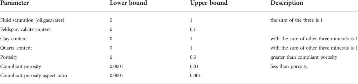
TABLE 1. Sampling range of conventional sandstone model parameters.
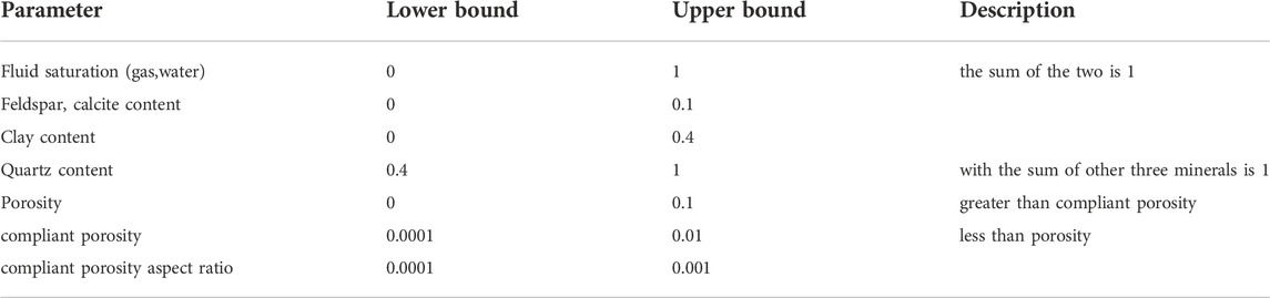
TABLE 2. Sampling range of tight sandstone model parameters.
Since real field data normally contain noise from the data acquisition, processing and interpretation procedures, we add 10% Gaussian noise to the synthetic data to construct a full-sample labeled dataset that mimics the real data, which helps enhance the robustness of the neural network.
The reservoir parameters reflect the characteristics of the reservoir, and there is a certain connection between them and the S-wave velocity. Since the trained neural network is to be directly applied to the real field work area, four reservoir parameters, such as porosity, density, clay content and P-wave velocity, which are easily accessible in real field areas, are selected. The correlation between the four parameters and the S-wave velocity is as follows (see Figure 1), where R is the correlation coefficient.
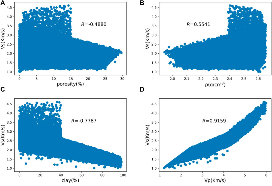
FIGURE 1. Correlation between reservoir parameters and S-wave velocity. (A) Porosity versus S-wave velocity. (B) Density versus S-wave velocity. (C) Clay content versus S-wave velocity. (D) P-wave velocity versus S-wave velocity.
According to the correlation analysis in Figure 1, it can be found that these four parameters have a good correlation with the S-wave velocity. The P-wave velocity and density are positively correlated with the S-wave velocity, and the porosity and clay content are negatively correlated with the S-wave velocity, among which the P-wave velocity has the strongest correlation with the S-wave velocity, and the absolute values of the four correlation coefficients are greater than 0.4. Thus, these four parameters will be used as the input features of the S-wave velocity prediction network.
Feature normalization is an important step in deep learning. Since different features always have different amplitudes, units, and ranges, the features with high magnitudes will impose higher impact on networks. If the data is not processed to the same range, the network may not converge when it is trained, and the training time is long, giving more weight to features with larger values, which will limit the prediction accuracy of the regression equation. In order to eliminate this effect, it is necessary to normalize the features to the same scale. This study uses the min-max method to normalize the features, and the normalized data are all between 0 and 1, the expressions are as follows:
where
In this study, a fully connected neural network with three hidden layers (the number of hidden layer neurons is 10), four inputs and one output is constructed using the P-wave velocity, density, porosity and clay content as input features and the S-wave velocity as the label (see Figure 2). The neural network minimizes the mean square error between the label and the output by back propagation using the gradient descent method. The activation function chosen for this network is the Rectified linear unit (ReLU) function to increase the nonlinear characterization ability of the neural network, the optimization algorithm is Adam, and the loss function is the mean square error (MSE) function.
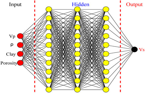
FIGURE 2. The structure of the deep S-wave velocity prediction network.
We use the full-sample labeled dataset constructed in Section 3.1 to train the deep shear velocity prediction network. Firstly, all the input features are normalized by the max-min method so that all the features fall between 0 and 1. Then 80% of the labeled dataset is used for training, 10% for validation and 10% for testing. As shown in Figure 3, the training and validation losses decrease simultaneously and converge to relatively low values after 14 epochs of training, which means that the neural network has been fitted well. The validation loss reaches a global minimum after 25 epochs and is as low as the training loss, indicating that the network has been completely fitted and the trained neural network can be generalized to new data for S-wave velocity prediction.
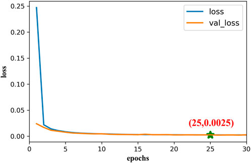
FIGURE 3. Learning curve of neural network.
For the trained network, the synthetic data with noise were first tested, and the test results are shown in Figure 4. From Figure 4A, it can be seen that the predicted S-wave velocity using the neural network can match the real S-wave velocity well both in terms of variation trend and values, except for individual data points where the error can reach more than 10%, the error in all other data points is below 5% (see Figure 4B).
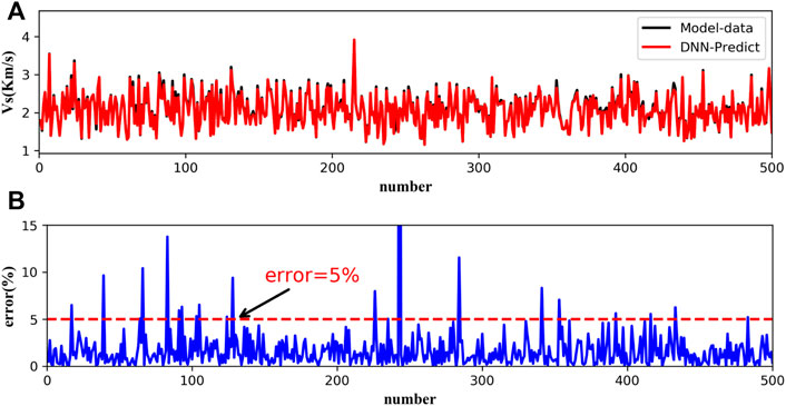
FIGURE 4. Test results of 500 synthetic data. (A) Test results. (B) Relative errors.
In this section we present the results of applying the neural network to laboratory data and real field data.
We obtained the clay content, porosity, density, P-wave velocity and S-wave velocity (dry conditions) of five tight sandstone samples from the published literature (Li et al., 2018; Han et al., 2021). The physical parameters of the five sandstone samples are shown in Table 3, and the P- and S-wave velocities are shown in Figure 5. Four features data from the published literature are introduced into the previously trained network and then output the predicted S-wave velocities.
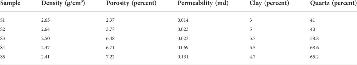
TABLE 3. petrophysical parameters of five tight sandstone samples.
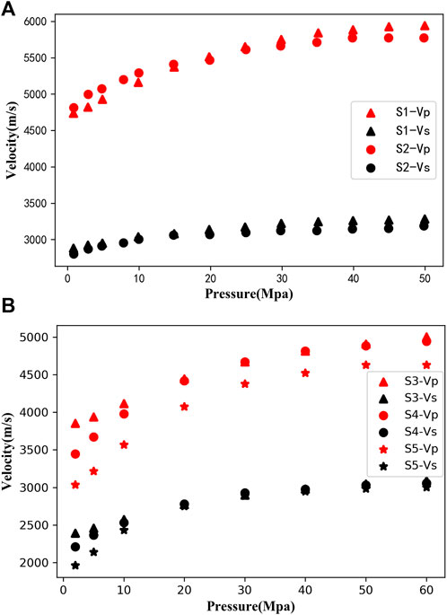
FIGURE 5. P- and S-wave velocities of samples from published literatures. (A) Han et al. (2021). (B) Li et al. (2018).
As shown in Figure 6A, the data are concentrated around the line y = x. The coefficient of certainty R2 of the prediction results is above 0.85, and the root mean square error (RMSE) is 0.12, indicating that the predicted S-wave velocities of the neural network are in strong agreement with the laboratory measurements. Most of the relative errors between the predicted results and experimental measurements are within 5% (see Figure 6B), which also indicates that the constructed deep S-wave velocity prediction network has a very good prediction performance, while the large deviation of individual points may be due to some errors generated by the experimental measurement process, resulting in low or high measured values.
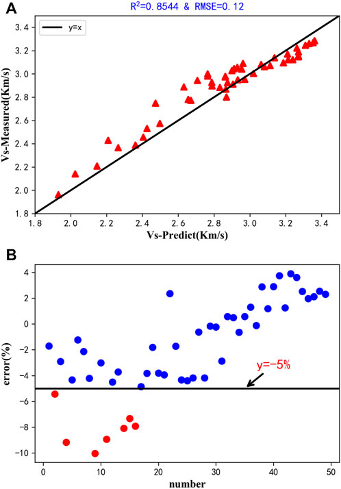
FIGURE 6. Comparison of S-wave velocity measured in laboratory with predicted value of DNN. (A) Prediction results. (B) Relative errors.
To illustrate the superiority of the constructed deep S-wave velocity prediction network, the predicted results of the network were compared with those predicted by the empirical formula proposed by Han et al. (1986), Eq. 12 and by Castagna et al. (1985), Eq. 13.
The comparison results and the average relative errors are shown in Figure 7. Figure 7A shows the two-dimensional intersection of the S-wave velocities predicted by the three methods and the laboratory measured S-wave velocities, and Figure 7B shows the relative errors. From Figure 7A, we can see that the intersection analysis results of the predicted and true values of the three methods are all distributed around the line y = x, which indicates that the prediction results have certain accuracy. However, the value predicted by the deep S-wave velocity prediction network is closer to the line y = x, which indicates that the network is the most accurate among the three methods. The errors between the predicted and true values of the network are the smallest, as can be seen in Figure 7B, which also confirm this conclusion. Also, it can be found from the figure that Han’s empirical formula is more applicable than Castagna’s empirical formula at the ultrasonic frequency band in the laboratory.
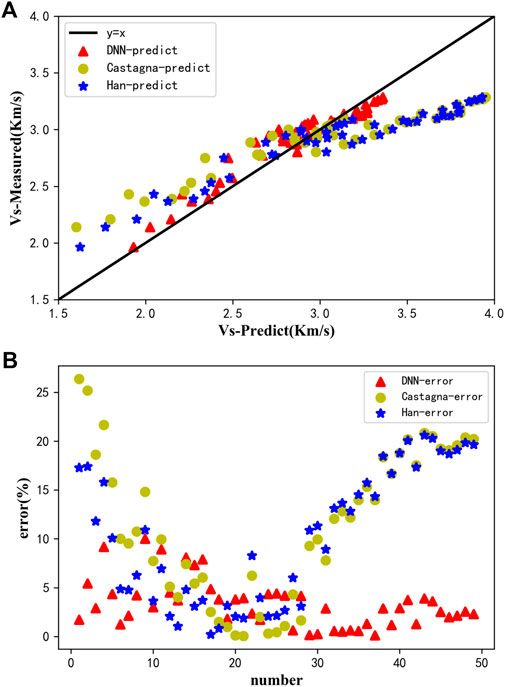
FIGURE 7. Comparison of three S-wave velocity prediction methods. (A) Prediction results. (B) Relative errors.
For tight sandstone, the P-wave velocity increases with increasing water saturation under high pressure conditions, and the S-wave velocity basically does not change, while both P-wave velocity and S-wave velocity increase with increasing water saturation under low pressure conditions (Li et al., 2018). Han’s empirical formula is obtained by fitting the saturated water sandstone data, while the data obtained in this study are measured under dry conditions, therefore, Han’s empirical formula results in a large prediction of the S-wave velocity under high pressure conditions (Figure 7A), while the prediction results of the S-wave velocity under low pressure conditions are very close to the true values.
The trained neural network was applied to the well log data from three real field areas for S-wave velocity prediction, where well 1 and well 2 were tight sandstone reservoirs and conventional sandstone reservoirs, while well 3 included both sandstone reservoirs and mudstone layers, and the results predicted by the deep S-wave velocity prediction neural network were compared with the real well log data and the results predicted by empirical formulas. The prediction results are shown in Figures 8–10, which show the logging data used in the prediction task as well as the prediction results and relative errors for the three methods. In Figures 8–10, Vs-label indicates real log shear wave velocity (black line), DNN-predict indicates the DNN prediction result (red line), Han-predict indicates the prediction result of Han’s empirical formula (blue line), Castagna-predict indicates the prediction result of Castagna’s empirical formula (yellow line), and Table 4 shows the average relative errors of the prediction results.
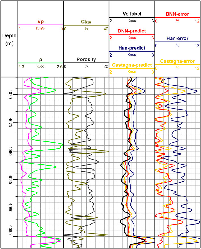
FIGURE 8. Data information of well 1 and S-wave velocity prediction results (Vs-label is the logging S-wave velocity, xx-predict indicates the result predicted using a certain method, and xx-error indicates the corresponding relative error).
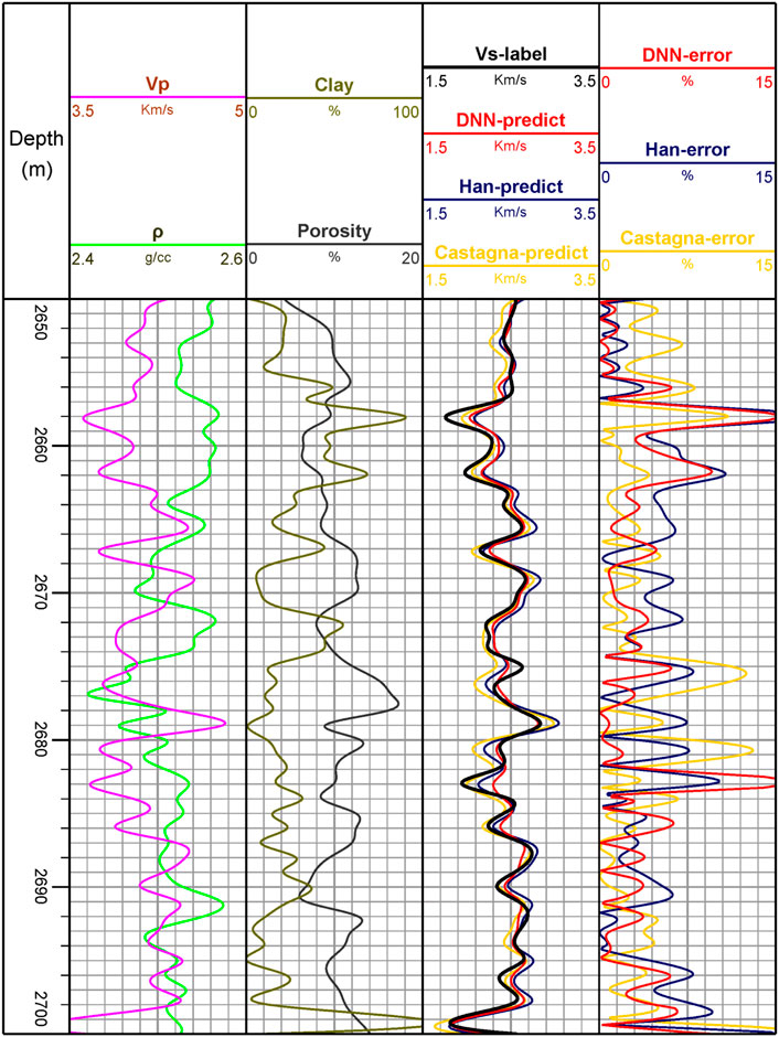
FIGURE 9. Data information of well 2 and S-wave velocity prediction results (Vs-label is the logging S-wave velocity, xx-predict indicates the result predicted using a certain method, and xx-error indicates the corresponding relative error).
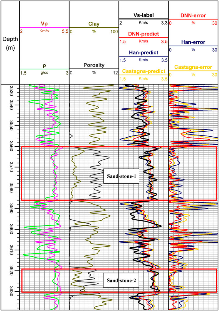
FIGURE 10. Data information of well 3 and S-wave velocity prediction results (Vs-label is the logging S-wave velocity, xx-predict indicates the result predicted using a certain method, and xx-error indicates the corresponding relative error).
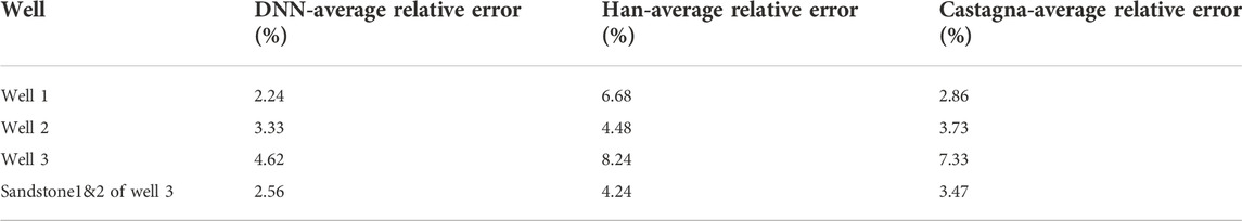
TABLE 4. Average relative error of the three S-wave velocity prediction methods in different wells.
From Figures 8, 9 and Table 4, we can see that for both Well one and Well 2, the S-wave velocity prediction results of the deep neural network and the real log data have the same general trend and small error, which has a good match. Compared with the other two prediction methods, the error of the DNN prediction results is smaller (2.24%, 3.33%) and the trend is closer to the real S-wave velocity, which indicates that the established deep S-wave velocity prediction network has good application in the real field work areas.
For well 3, the deep neural network prediction results are relatively poor, but from Figure 10 and Table 4, we can see that the deep neural network still performs well in the two sandstone reservoir sections (2.56%), while the prediction results of the mudstone section deviate greatly from the true values. This is owing to the fact that the rock physic responses of mudstone are different from that of both tight sandstone and conventional sandstone, and the labeled dataset constructed by the sandstone model is less applicable to mudstone, so there exists a large prediction error. In addition, the prediction accuracy of the deep neural network is also superior to the two empirical formulations, the same as the results of wells 1 and 2, because this high clay content is taken into account in the sandstone modeling process. Figures 8–10 and Table 4 also show that Castagna’s empirical formula is more applicable than Han’s empirical formula at the well-logging frequency band.
Figure 11 shows the absolute error (the absolute value of the difference between the measured and predicted S-wave velocities) of the S-wave velocities predicted based on the deep neural network for the three wells. As can be seen from the figure, the absolute error is basically below 0.15 km/s for well 1, and below 0.2 km/s for well 2 as well as the sandstone section of well 3, which indicates that the practicality of the method proposed in this study is fairly good.
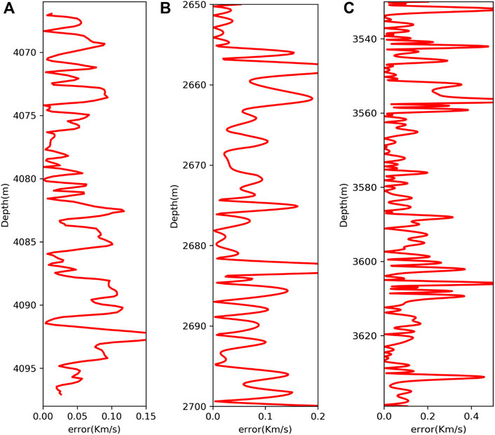
FIGURE 11. Absolute error curve of S-wave velocity predicted by DNN. (A) Well 1. (B) Well 2. (C) Well 3.
From the application of the laboratory data and the well log data, the prediction accuracy of the deep S-wave velocity prediction network established in this study is higher than the common empirical formulas. Han’s empirical formula is more applicable to the ultrasonic frequency band, while Castagna’s proposed empirical formula is more applicable to the well-logging frequency band, which may be because Han’s empirical formula is statistically based on the data at ultrasonic frequency band, while Castagna’s empirical formula is based on the well-logging data. Compared with the two empirical formulations, the deep S-wave velocity prediction network proposed in this study is applicable to the full frequency band S-wave velocity prediction and has better generalization.
In this study, we proposed a shear wave velocity prediction method based on DNNs and rock physics modeling. We have applied the established deep S-wave velocity prediction network to real field data directly. Theoretical rock physics models are developed for the properties of conventional and tight sandstone reservoirs. The geological and geophysical knowledge is incorporated into the data set of the deep neural network by means of forwarding simulation of the theoretical rock physics models to construct a full-sample labeled dataset that traverses the entire S-wave velocity space. A robust and generalizable deep S-wave velocity prediction network without multiple training is built by combining the full-sample labeled dataset and the deep neural network. When the established network is applied to the real field data, the errors of S-wave velocity prediction are very small, all within 200 m/s, and the average relative errors are below 5%. In addition, the prediction errors of the deep S-wave velocity prediction network constructed in this study applied to laboratory data (3.32%) and well log data (2.24, 3.33, and 4.62%) are much smaller than that of Han’s empirical formula (10.30, 6.68, 4.48, and 8.24%) and Castagna’s empirical formula (11.40, 2.86, 3.73, and 7.33%). Compared with the two common empirical formulations, the deep S-wave velocity prediction network established has better prediction ability and generalization ability. The network is applicable to the S-wave velocity prediction in the full frequency band of sandstone reservoirs, and can provide S-wave velocity information for reservoir prediction work. The use of theoretical model forward simulation supplements the training dataset for machine learning, improving the interpretability of machine learning algorithms and generalization of models in real applications. Furthermore, we provide a new idea for the construction of labeled datasets in machine learning tasks.
The raw data supporting the conclusion of this article will be made available by the authors, without undue reservation.
GF: acquisition and processing of data, methodology, manuscript writing and revising; H-HZ: manuscript reviewing and editing; X-RX: manuscript editing; G-YT: the conception and design of the study; Y-XW: provide some suggestions.
This study was supported by the Research on Full-Frequency Processing Method of Thin Reservoir and Research on Target Fine Characterization Technology Research (2022KT1503), the Research on Geophysical Description Technology of Continental Clastic Reservoir and Field Test (2022KT1505), the NSFC program (41930425) and the CNPC-CUPB Strategic Corporation Science and Technology Program (ZLZX2020-03).
Authors GF, H-HZ, X-RX, and Y-XW were employed by PetroChina.
The remaining author declares that the research was conducted in the absence of any commercial or financial relationships that could be construed as a potential conflict of interest.
All claims expressed in this article are solely those of the authors and do not necessarily represent those of their affiliated organizations, or those of the publisher, the editors and the reviewers. Any product that may be evaluated in this article, or claim that may be made by its manufacturer, is not guaranteed or endorsed by the publisher.
Alimoradi, A., Shahsavani, H., and Rouhani, A. K. (2011). Prediction of shear wave velocity in underground layers using SASW and artificial neural networks. Engineering 3 (03), 266–275. doi:10.4236/eng.2011.33031
Ameen, M. S., Smart, B., Somerville, J. M., Hammilton, S., and Naji, N. A. (2009). Predicting rock mechanical properties of carbonates from wireline logs (A case study: Arab-D reservoir, Ghawar field, Saudi Arabia). Mar. Pet. Geol. 26 (4), 430–444. doi:10.1016/j.marpetgeo.2009.01.017
Bagheripour, P., Gholami, A., Asoodeh, M., and Vaezzadeh-Asadi, M. (2015). Support vector regression based determination of shear wave velocity. J. Petroleum Sci. Eng. 125, 95–99. doi:10.1016/j.petrol.2014.11.025
Biot, M. A. (1956). Theory of propagation of elastic waves in a fluid-saturated porous solid. I. Low-Frequency range. J. Acoust. Soc. Am. 28 (2), 168–178. doi:10.1121/1.1908239
Castagna, J. P., Batzle, M. L., and Eastwood, R. L. (1985). Relationships between compressional-wave and shear-wave velocities in clastic silicate rocks. Geophysics 50 (4), 571–581. doi:10.1190/1.1441933
Du, X. (2014). Shear wave velocity delicate estimation based on Trivariate Cauchy constraint AVO inversion. Prog. Geophys. 29 (2), 681–688. doi:10.6038/pg20140228
Dvorkin, J., Mavko, G., and Nur, A. (1995). Squirt Flow in fully saturated rocks. Geophysics 60 (1), 97–107. doi:10.1190/1.1443767
Eberhart-Phillips, D., Han, D. H., and Zoback, M. D. (1989). Empirical relationships among seismic velocity, effective pressure, porosity, and clay content in sandstone. Geophysics 54 (1), 82–89. doi:10.1190/1.1442580
Eskandari, H., Rezaee, M. R., and Mohammadnia, M. (2004). Application of multiple regression and artificial neural network techniques to predict shear wave velocity from wireline log data for a carbonate reservoir South-West Iran. CSEG Rec. 42, 48.
Gao, J., Song, Z., Gui, J., and Yuan, S. (2022). Gas-bearing prediction using transfer learning and CNNs: An application to a deep tight dolomite reservoir. IEEE Geosci. Remote Sens. Lett. 19, 1–5. doi:10.1109/LGRS.2020.3035568
Gassmann, F. (1951). Elastic waves through a packing of spheres. Geophysics 16 (4), 673–685. doi:10.1190/1.1437718
Guo, W., Dong, C., Lin, C., Wu, Y., Zhang, X., and Liu, J. (2022). Rock physical modeling of tight sandstones based on digital rocks and reservoir porosity prediction from seismic data. Front. Earth Sci. (Lausanne). 10, 932929. doi:10.3389/feart.2022.932929
Guo, Z., Qin, X., Zhang, Y., Niu, C., Wang, D., and Ling, Y. (2021). Numerical investigation of the effect of heterogeneous pore structures on elastic properties of tight gas sandstones. Front. Earth Sci. (Lausanne). 9, 641637. doi:10.3389/feart.2021.641637
Gurevich, B., Makarynska, D., De Paula, O. B., and Pervukhina, M. (2010). A simple model for squirt-flow dispersion and attenuation in fluid-saturated granular rocks. Geophysics 75 (6), N109–N120. doi:10.1190/1.3509782
Han, D., Nur, A., and Morgan, D. (1986). Effects of porosity and clay content on wave velocities in sandstones. Geophysics 51 (11), 2093–2107. doi:10.1190/1.1442062
Han, X., Wang, S., Tang, G., Dong, C., He, Y., Liu, T., et al. (2021). Coupled effects of pressure and frequency on velocities of tight sandstones saturated with fluids: Measurements and rock physics modelling. Geophys. J. Int. 226 (2), 1308–1321. doi:10.1093/gji/ggab157
Hill, R. (1952). The elastic behaviour of a crystalline aggregate. Proc. Phys. Soc. A 65 (5), 349–354. doi:10.1088/0370-1298/65/5/307
Hu, C., Wang, F., and Ai, C. (2021). Calculation of average reservoir pore pressure based on surface displacement using image-to-image convolutional neural network model. Front. Earth Sci. (Lausanne). 9, 712681. doi:10.3389/feart.2021.712681
Hu, R., Peng, Z., Ma, J., and Li, W. (2020). CNN-based vehicle target recognition with residual compensation for circular SAR imaging. Electronics 9 (4), 555. doi:10.3390/electronics9040555
Kuster, G. T., and Toksőz, M. N. (1974). Velocity and attenuation of seismic waves in two-phase media:Part I. Theoretical formulations. Geophysics 39 (5), 587–606. doi:10.1190/1.1440450
Li, D., Wei, J., Di, B., Ding, P., Huang, S., and Shuai, D. (2018). Experimental study and theoretical interpretation of saturation effect on ultrasonic velocity in tight sandstones under different pressure conditions. Geophys. J. Int. 212 (3), 2226–2237. doi:10.1093/gji/ggx536
Maleki, S., Moradzadeh, A., Riabi, R. G., Gholami, R., and Sadeghzadeh, F. (2014). Prediction of shear wave velocity using empirical correlations and artificial intelligence methods. NRIAG J. Astronomy Geophys. 3 (1), 70–81. doi:10.1016/j.nrjag.2014.05.001
Mehrgini, B., Izadi, H., and Memarian, H. (2017). Shear wave velocity prediction using Elman artificial neural network. Carbonates Evaporites 34 (4), 1281–1291. doi:10.1007/s13146-017-0406-x
Sun, S. Z., Wang, H., Liu, Z., Li, Y., Zhou, X., and Wang, Z. (2012). The theory and application of DEM-Gassmann rock physics model for complex carbonate reservoirs. Lead. Edge 31 (2), 152–158. doi:10.1190/1.3686912
Wang, J., Cao, J., Zhao, S., and Qi, Q. (2022). S-wave velocity inversion and prediction using a deep hybrid neural network. Sci. China Earth Sci. 65 (4), 724–741. doi:10.1007/s11430-021-9870-8
White, J. E. (1975). Computed seismic speeds and attenuation in rocks with partial gas saturation. Geophysics 40 (2), 224–232. doi:10.1190/1.1440520
Wu, X., Geng, Z., Shi, Y., Pham, N., Fomel, S., and Caumon, G. (2019). Building realistic structure models to train convolutional neural networks for seismic structural interpretation. Geophysics 85 (4), WA27–WA39. doi:10.1190/geo2019-0375.1
Xu, S., and Payne, M. A. (2009). Modeling elastic properties in carbonate rocks. Lead. Edge 28 (1), 66–74. doi:10.1190/1.3064148
Xu, S., and White, R. E. (1995). A new velocity model for clay-sand mixtures 1. Geophys. Prospect. 43 (1), 91–118. doi:10.1111/j.1365-2478.1995.tb00126.x
Xu, S., and White, R. E. (1996). A physical model for shear-wave velocity prediction. Geophys. Prospect. 44 (4), 687–717. doi:10.1111/j.1365-2478.1996.tb00170.x
Yu, S., and Ma, J. (2021). Deep learning for geophysics: Current and future trends. Rev. Geophys. 59 (3), e2021RG000742. doi:10.1029/2021RG000742
Yuan, S., Jiao, X., Luo, Y., Sang, W., and Wang, S. (2022). Double-scale supervised inversion with a data-driven forward model for low-frequency impedance recovery. Geophysics 87 (2), R165–R181. doi:10.1190/geo2020-0421.1
Yuan, S., Liu, J., Wang, S., Wang, T., and Shi, P. (2018). Seismic waveform classification and first-break picking using convolution neural networks. IEEE Geosci. Remote Sens. Lett. 15 (2), 272–276. doi:10.1109/LGRS.2017.2785834
Zhang, Y., Zhang, C., Ma, Q., Zhang, X., and Zhou, H. (2022). Automatic prediction of shear wave velocity using convolutional neural networks for different reservoirs in Ordos Basin. J. Petroleum Sci. Eng. 208, 109252. doi:10.1016/j.petrol.2021.109252
Keywords: deep neural network, rock physics modeling, theoretical rock physics model, full-sample labeled dataset, shear wave velocity prediction, empirical formula
Citation: Feng G, Zeng H-H, Xu X-R, Tang G-Y and Wang Y-X (2023) Shear wave velocity prediction based on deep neural network and theoretical rock physics modeling. Front. Earth Sci. 10:1025635. doi: 10.3389/feart.2022.1025635
Received: 23 August 2022; Accepted: 20 October 2022;
Published: 11 January 2023.
Edited by:
Xiaolan Qiu, Aerospace Information Research Institute (CAS), ChinaCopyright © 2023 Feng, Zeng, Xu, Tang and Wang. This is an open-access article distributed under the terms of the Creative Commons Attribution License (CC BY). The use, distribution or reproduction in other forums is permitted, provided the original author(s) and the copyright owner(s) are credited and that the original publication in this journal is cited, in accordance with accepted academic practice. No use, distribution or reproduction is permitted which does not comply with these terms.
*Correspondence: Gen-Yang Tang, dGFuZ2dlbnlhbmdAMTYzLmNvbQ==
Disclaimer: All claims expressed in this article are solely those of the authors and do not necessarily represent those of their affiliated organizations, or those of the publisher, the editors and the reviewers. Any product that may be evaluated in this article or claim that may be made by its manufacturer is not guaranteed or endorsed by the publisher.
Research integrity at Frontiers
Learn more about the work of our research integrity team to safeguard the quality of each article we publish.