 Guozhong Gao1,2
 Omid Hazbeh3
 Shadfar Davoodi4Somayeh Tabasi5
 Meysam Rajabi6
 Hamzeh Ghorbani7,8*
 Ahmed E. Radwan9Mako Csaba10
 Amir H. Mosavi11*
- 1College of Geophysics and Petroleum Resources, Yangtze University, Wuhan, Hubei, China
- 2Cooperative Innovation Center of Unconventional Oil and Gas, Yangtze University (Ministry of Education & Hubei Province), Wuhan, Hubei, China
- 3Faculty of Earth Sciences, Shahid Chamran University, Ahwaz, Iran
- 4School of Earth Sciences and Engineering, Tomsk Polytechnic University, Tomsk, Russia
- 5Faculty of Industry and Mining (Khash), University of Sistan and Baluchestan, Zahedan, Iran
- 6Department of Mining Engineering, Birjand University of Technology, Birjand, Iran
- 7Young Researchers and Elite Club, Ahvaz Branch, Islamic Azad University, Ahvaz, Iran
- 8Faculty of General Medicine, University of Traditional Medicine of Armenia (UTMA), Yerevan, Armenia
- 9Faculty of Geography and Geology, Institute of Geological Sciences, Jagiellonian University, Kraków, Poland
- 10Independent Researcher, Budapest, Hungary
- 11Independent Researcher, Kyiv, Ukraine
One of the challenges that reservoir engineers, drilling engineers, and geoscientists face in the oil and gas industry is determining the fracture density (FVDC) of reservoir rock. This critical parameter is valuable because its presence in oil and gas reservoirs boosts productivity and is pivotal for reservoir management, operation, and ultimately energy management. This valuable parameter is determined by some expensive operations such as FMI logs and core analysis techniques. As a result, this paper attempts to predict this important parameter using petrophysics logs routinely collected at oil and gas wells and by applying four robust computational algorithms and artificial intelligence hybrids. A total of 6067 data points were collected from three gas wells (#W1, #W2, and #W3) in one gas reservoir in Southwest Asia. Following feature selection, the input variables include spectral gamma ray (SGR); sonic porosity (PHIS); potassium (POTA); photoelectric absorption factor (PEF); neutron porosity (NPHI); sonic transition time (DT); bulk density (RHOB); and corrected gamma ray (CGR). In this study, four hybrids of two networks were used, including least squares support vector machine (LSSVM) and multi-layer perceptron (MLP) with two optimizers particle swarm optimizer (PSO) and genetic algorithm (GA). Four robust hybrid machine learning models were applied, and these are LSSVM-PSO/GA and MLP-PSO/GA, which had not previously used for prediction of FVDC. In addition, the k-fold cross validation method with k equal to 8 was used in this article. When the performance accuracy of the hybrid algorithms for the FVDC prediction is compared, the revealed result is LSSVM-PSO > LSSVM-GA > MLP-PSO > MLP-GA. The study revealed that the best algorithm for predicting FVDC among the four algorithms is LSSVM-PSO (for total dataset RMSE = 0.0463 1/m; R2 = 0.9995). This algorithm has several advantages, including: 1) lower adjustment parameters, 2) high search efficiency, 3) fast convergence speed, 4) increased global search capability, and 5) preventing the local optimum from falling. When compared to other models, this model has the lowest error.
Introduction
One of the challenges that reservoir management, drilling, and exploitation of oil and gas resources, and finally energy management have always faced is achieving decent productivity with the least amount of cost (Zheng et al., 2017; Abad et al., 2022). One of the most important reservoirs in the oil and gas industry is natural fracture reservoirs. These reservoirs are among the special reservoirs that change the fluid flow regime of the reservoirs and affect the well productivity (Yang et al., 2018; Radwan et al., 2021). Sometimes, in some areas, the presence of deep fractures causes water conning in these areas, and undesirable fluids flow to less permeable areas, where they are wasted in the subsurface (Ali et al., 2021; Sadeghnejad et al., 2022). Many techniques have been used to identify fracture density. Among these techniques, coring operations are crucial to identify reservoir rock fractures (Rajabi et al., 2021; Sipahi and Develi, 2021). This operation is so costly that it is done only in some limited reservoirs and is extremely rare (Bessa et al., 2021). This paper attempts to use low-cost petrophysical logs, which are required in all wells as part of the drilling process, as well as four newly developed artificial intelligence hybrid algorithms. The fracture density parameter (FVDC) can be defined as the number of fractures per unit length for a rock unit in cumulative fractures per unit volume. This parameter can be extracted from visual reports, and it can be written in the following formula (Lai et al., 2017):
In recent years, artificial intelligence has grown dramatically, and many people have used it to predict important parameters in various fields (Ahmadi et al., 2020; Nabipour et al., 2020b; Nourani et al., 2022). Previous research has made some progress in fracture prediction using artificial intelligence, including the following:
Initially, Ince (2004) used four inputs for fracture prediction using Young’s modulus (E), compressive strength (fc), water-cation ration (w/c) and maximum aggregate size (dmax), using 40 data points. Cement failure information is predicted using a neural network (ANN) algorithm. Based on the results, it was found that this algorithm has a very high capability in fracture detection and cement fracture prediction (Ince, 2004). Six years after Mr. Ince’s work, Jafari et al. (2012) predicted fracture density using data from fifteen wells in the Asmari Formation, southwestern Iran. In Jafari’s paper, bulk density (RHOB), deep resistance (RT), and neutron porosity were used as input data to predict this important parameter using an adaptive neuro-fuzzy inference system (ANFIS) (NPHI). The presented results indicate that this algorithm has a high prediction accuracy, with R2 = 0.98 and Error = 16.2, indicating that it has a low error (Ja’fari et al., 2012). One year after the work of Jafari et al. (2012), Zazoun (2013) used the robust ANN algorithm to predict fracture density. A total of 1349 data points from 17 wells in the Mesdar oil field in Algeria were used for this purpose. The input data used in Zazoun’s paper to predict this important parameter include RHOB, sonic transient time (DT), Caliper, depth (D), NPHI, and gamma ray (GR). The presented results indicate the high accuracy of this algorithm with a value of R2 = 0.812 (Zazoun, 2013). Two years after Zazoun’s work, in 2015, Nouri-Taleghani et al. (2015) used the robust committee machine intelligent system (CIMS) algorithm to predict fracture density. For this purpose, they used 395 data points from the Marun oil field, Iran. The input data used in Nouri-Taleghani’s work to predict this important parameter includes: RHOB, depth (D), caliper (HS), NPHI, photoelectric absorption factor (PEF), and induced deep resistivity log(ILD). The presented results indicate the high accuracy of this algorithm with a value of R2 = 0.895 and the value of Error = 10.2 (Nouri-Taleghani et al., 2015). Three years after Nouri-Taleghani’s work, in 2018, Bhattacharya and Mishra (2018) used strong bayesian belief network (BN) and random forest (RF) algorithms to predict fracture density. For this purpose, they used 395 data points from the Appalachian basin, United States. Input variables to predict this important parameter include RHOB, GR, and HS absorption. The presented results indicate the high accuracy of this algorithm, and the absolute accuracy is between 74.8% and 79.6%.
Away from direct observations from cores, numerous methods for diagnosing and determining fractures in subsurface reservoirs have been proposed. One of the methods is fluid loss recordings during drilling, which can reveal fractures in the subsurface rocks. It should be noted that natural fractures are not always useful can result in drilling fluid waste and other issues. However, the fluid loss does not accurately determine the extent of the fracture. Another advanced method of fracture diagnosis is the process of fracture detection using image logs (FMI), which is very expensive. Computed Tomography (CT) scanning for determining a reservoir’s fracture network in three dimensions. However, it is a very costly and time-consuming operation.
The LSSVM is one of the most powerful estimation modeling tools that has been widely used by researchers to model complex problems. As a result, combining LSSVM with ultra-innovative algorithms such as PSO and GA has demonstrated that it can dramatically improve the accuracy of the output model. Therefore, we used LSSVM-PSO and LSSVM-GA hybrid algorithms. This study tries to develop four robust hybrid machine learning algorithms and employs eight input variables related to petrophysical logs that have not previously been used together in the literature. In this article, four ML algorithms were used: MLP-PSO/GA and LSSVM-PSO/GA. To the best of our knowledge, these algorithms have been used in other industrial problems, but they have not yet been used to investigate the fracture density incident. Table 1 shows the merits and disadvantages of the algorithms. In addition, in this study, information about petrophysical logs and FMI logs (FVDC determination) was used for input and output, respectively.
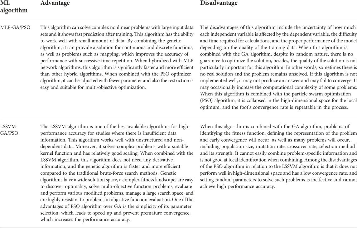
TABLE 1. Compare the advantage and disadvantages of hybrid machine learning algorithms used for FVDC prediction.
Methodology
The diagram in Figure 1 shows the steps of building, completing, and evaluating four robust HML algorithms to predict FVDC. As shown in this Figure 1, we began by collecting data from three wells (#W1, #W2, and #W3) in a gas reservoir located in Southwest Asia. In the next step, the maximum and minimum values of each variable are specified, and then the data of all variables are normalized between -1 and +1 (based on Eq. 2).
Where:
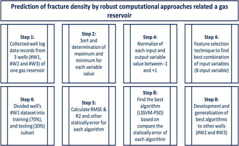
FIGURE 1. Flow diagram for workflow chart to develop four robust hybrid machine learning models for prediction of FVDC.
Initially, the number of input variables was 12, but after feature selection, this number was reduced to 8. Finally, the well data from well #W1 is divided into training (70%) and testing (30%) categories, and four new AI hybrid algorithms are developed. We compared the algorithms’ results using statical parameters and finally selected the best algorithm and generalized the best hybrid algorithm (LSSVM-PSO) using the other two wells #W2 and #W3, and the results were confirmed.
Due to their powerful capability to map correlation among data and find solution for different problems, ML models’ application has become much popular in various fields of science and engineering over the last few decades (Choubin et al., 2019; Ghalandari et al., 2019; Qasem et al., 2019; Torabi et al., 2019; Ahmadi et al., 2020; Band et al., 2020; Mosavi et al., 2020; Shabani et al., 2020; H Ghorbani and Davarpanah, 2021). For instance, ML methods have been applied for tackling a variety of challenges in petroleum engineering such as petrophysical (Rajabi et al., 2022c; Jafarizadeh et al., 2022; Tabasi et al., 2022; Zhang et al., 2022), reservoir characterization (Hassanpouryouzband et al., 2020; Abad et al., 2021a; Hassanpouryouzband et al., 2021; Zhang et al., 2021; Kamali et al., 2022; Kamali et al., 2022; Rajabi et al., 2022d; Hassanpouryouzband et al., 2022; Ibrahim et al., 2022; Zhang et al., 2022), production (Mirzaei-Paiaman and Salavati, 2012; Ghorbani et al., 2020; Abad et al., 2021b) drilling (Soares and Gray, 2019; Syah et al., 2021; Beheshtian et al., 2022; Pang et al., 2022). To predict fracture density using conventional well logs in this study, two ML algorithms, multi-Layer Perceptron’s and least-squares support-vector machines, were combined with two evolutionary optimizers: genetic algorithm and particle swarm optimization. One reason for choosing MLP and LSSVM to predict FVDC is that the MLP algorithm is very flexible and can form a suitable mapping to learn the pattern of input variables to determine FVDC and provide an acceptable result. The Least Squares Support Vector Algorithm (LS-SVM) analyzes input data using a set of supervised learning methods and performs regression analysis by identifying the appropriate pattern. In order to optimize and increase the performance accuracy of the algorithms, we have used GA and PSO optimizers. The advantages and disadvantages of the algorithms are presented in Table 1.
Multi-layer perceptron’s model
An artificial neural network (ANN) is an intelligent tool used for establishing complex non-linear relationships between a set of variables. As a result, ANN can predict the dependent (output) variable(s) of interest with high accuracy (Barjouei et al., 2021). There are various types of neural networks that have been widely employed in the energy industry and other industries (Taherei Ghazvinei et al., 2018; Ghalandari et al., 2019; Nabipour et al., 2020b; Shamshirband et al., 2020). To develop a high-efficiency ANN model, several key factors must be considered: 1) network architecture (number of nodes and layers), 2) transfer functions applied between layers, 3) selection of training algorithm used for optimizing the prediction performance, and 4) selection of proper features (i.e., which independent variables to consider). It should be mentioned that the aforementioned factors play a vital role in determining the degree of prediction accuracy of ANN models (Maimon and Rokach, 2005). The MLP algorithm is regarded as the most important type of artificial neural network, and it consists of one input and one output layer, as well as one or more layers between the input and output layers known as “hidden layer(s)”. Being trained in a supervised manner by the back propagation algorithm, MLP has been extensively used in solving a wide range of problems (Rady and Anwar, 2019). The MLP algorithm is applied for dealing with large and complex sets of data as a flexible and versatile ANN (Bishop and Nasrabadi, 2006). Consequently, the MLP model was chosen in the present work for FVDC prediction.
A three-hidden-layer structure was found to be the optimal structure for the MLP model evaluated in this study after a trial-and-error analysis. The number of nodes within hidden layers was equal to eight, ten, and one for the 1st, 2nd, and 3rd layers, respectively. Based on the trial-and-error analysis, “tansig”, “purelin” and “tansig” were selected as transfer functions for the 1st, 2nd, and 3rd layers, respectively. Although Levenberg-Marquardt (LM) algorithm is the most commonly applied for MLP training due to its performance in rapid convergence to optimal solutions. However, when dealing with large complex non-linear datasets, this algorithm suffers strongly from trapping at local minima (Nawi et al., 2014). To tackle this challenge, PSO and GA algorithms were combined with MLP to enhance the global optimization of the developed models (MLP-GA and MLP-PSO).
Least-squares support-vector machines
In 1995, Vapink proposed a rubout ML algorithm with high efficiency called Support Vector Machine (Cortes and Vapnik, 1995). Since its inception, this supervised ML algorithm has been widely used to address regression and classification tasks. The SVM algorithm presents some advantages over neural network algorithms, including: 1) no network predetermination is required; 2) no need to determine the number of layers and neurons; 3) SVM requires fewer control parameters than ANN (Gholami and Fakhari, 2017). Despite these advantages, this ML technique involves a complex learning process that involves the implementation of a set of nonlinear equations solved via quadratic programming (Mahdaviara et al., 2020; Abad et al., 2021a). To address the learning complexity of SVM, some changes were made to the SVM algorithm by Suykens and Vandewalle in 1999 (Suykens and Vandewalle, 1999). The modified version of this technique is the least-squares support-vector machine (LSSVM). The LSSVM algorithm simplifies the learning process by solving a set of linear equations rather than complicated non-linear equations. In the LSSVM model, the approximation is performed using the following cost function (see Eq. 3) (Suykens et al., 2002).
where
Although the kernel function has a significant impact on the LS-SVM prediction performance, no standard methods have been proposed for its selection (Abad et al., 2021a; Rashidi et al., 2021). Therefore, for the LS-SVM model proposed in this study, four commonly used kernel functions, such as multilayer perceptron kernel, polynomial kernel, radial basis function (RBF) kernel, and linear kernel, were evaluated. The kernel function efficiency analysis displayed that the RBF kernel is outperformed all the four kernel functions tested. Furthermore, to boost the prediction performance of the LS-SVM model, GA and PSO optimizers were used to determine the optimum values of control parameters of the model proposed.
Optimization algorithms
Genetic algorithm
The Genetic Algorithm (GA) is a well-known multi-purpose optimization algorithm that is extensively used in a wide range of prediction issues (Holland, 1984). This optimization algorithm process mimics natural selection processes that involve population modification procedures. These processes include random mutation and crossover using a randomly selected population of individuals (Mitchell, 1998; Sivanandam and Deepa, 2008; Hassanat et al., 2019). The flowchart displayed in Figure 2 illustrates the execution procedure of the GA algorithm, adapted from Sivanandam and Deepa (2008). GA performs some adjustments to the population’s individuals based on the RMSE values they represent. The individual with the lowest value of RMSE is retained as the global best (Gb). Other individuals with sub-optimal values of RMSE are chosen for modifications to proceed further and enter to the next generation. Individuals who outperform those with high values of RMSE, are randomly replaced in the next generation. The overall population becomes gradually fitter and fitter through this sequence of natural selection and the Gb solution improves. The individuals are adapted via selection, mutation, or crossover as GA continues its iterations. The iterations are continued until, either a preset value of low RMSE is accomplished, or a specified number of iterations are carried out (Ashrafi et al., 2019; Mohamadian et al., 2021).
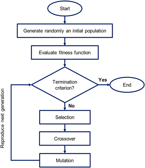
FIGURE 2. Flowchart diagram displaying the execution procedure for GA.
Particle swarm optimization
In 1995, Kennedy and Eberhart established a new evolutionary optimization algorithm based on the natural swarming of birds, called particle swarm optimization (PSO). In this optimizer, a population of random solutions “swarm”, is initiated, and an optimum solution then obtained by updating generation. The solutions, in this algorithm, are called “particles” (Abad et al., 2021a). The flowchart shown in Figure 3 presents the execution steps that are involved in the PSO algorithm, adapted from Rajabi et al. (2022b). This algorithm initializes a swarm of particles by specifying maximum (Vmax) and minimum values (Vmin). In each iteration of optimization, the best positions globally obtained by the swarm of particles (Gb) and the best positions achieved by the particles (Pb) are recorded and transferred to the next iteration (Kuo et al., 2010; Kıran et al., 2012). With reference to this information about the lowest Pb and Gb positions recorded, the velocity attributes of each particle are modified (see Eq. 4), adjusting its position as given by Eq. 5.
where
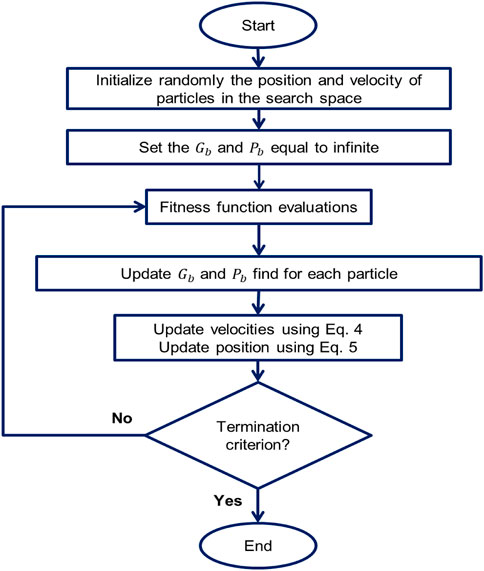
FIGURE 3. Flowchart diagram displaying the execution procedure for PSO.
Hybrid machine-learning models for fracture density prediction
Multi-layer perceptron-genetic algorithm/particle swarm optimizer models
Hybrid forms of MLP and LSSVM algorithms with PSO and GA optimizers have presented themselves as promising hybrid methods for diverse prediction purposes in different engineering sections, particularly in the oil and gas industry. For instance, these hybrid methods have shown significant accuracy in the prediction of different parameters, such as shear wave velocity (Ghorbani et al., 2021; Miah, 2021; Rajabi et al., 2022a), viscosity of waxy crude oils (Madani et al., 2021), estimating formation pore pressure (Rajabi et al., 2022b), safe mud window (Beheshtian et al., 2022), gas flow rate (Abad et al., 2022), casing collapse (Mohamadian et al., 2021), rock porosity and permeability (Nourani et al., 2022), two-phase flow pressure drop modelling (Faraji et al., 2022), rate of penetration in drilling (Hashemizadeh et al., 2022), gas condensate viscosity (Abad et al., 2021a), prediction based on biodiesel distillation (Vera-Rozo et al., 2022), oil holdup (Zhang et al., 2011). The promising accuracy achieved by the optimized LSSVM and MLP models for different prediction purposes trigged the idea to establish solid hybrid methods based on these algorithms and evaluate their performance in the FVDC prediction using conventional well logs.
The MLP algorithm was hybridized with GA and PSO optimizers to identify the optimum values of biases and weights applied to the MLP model, where two hybridized machine-learning models, namely MLP-GA and MLP-PSO, were established. Figure 4 illustrates the flowchart of the MLP-GA/PSO models, adapted from Zhang et al. (2022).
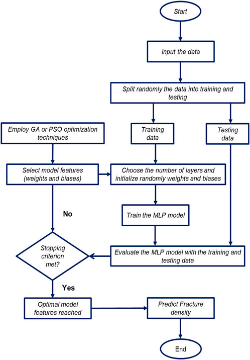
FIGURE 4. Flowchart for MLP-GA/PSO models used for prediction of fracture density.
The PSO optimizer applied has a setup of 60 particles with 100 iterations to reach the optimal solution. The setup of the GA optimizer used includes 60 populations with 100 iterations. The control parameters of the MLP-GA/PSO models used to predict fracture density are listed in Table 2.
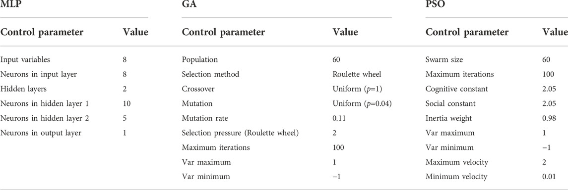
TABLE 2. Control parameters for MLP-GA/ PSO models used for the prediction of fracture density.
Least-squares support-vector machines -genetic algorithm/particle swarm optimizer models
Like the MLP algorithm, the LSSVM algorithm was hybridized either with GA or PSO optimization algorithms to identify the optimal values of its control parameters. Among all four kernel functions tested for the LSSVM model in the present work, the RBF kernel presents the best efficiency. The optimum values of control parameters for LSSVM, RBF kernel variance (
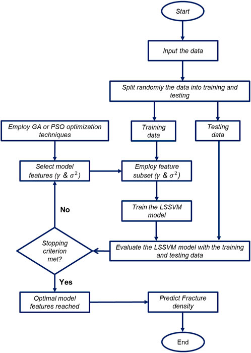
FIGURE 5. Flowchart for LSSVM-GA/PSO models used for prediction of fracture density.
Feature detection for fracture density prediction and cross validation
The performance speed and accuracy of the HML algorithms of MLP-PSO/GA and LSSVM-PSO/GA can be increased by selecting the best input variables that have the greatest impact on FVDC, which increases the performance accuracy of these algorithms. This method necessitates the use of the feature selection method and ranking input variables for accessibility in accordance with the 2N rule (N is the number of input variables) (Wahab et al., 2015; Beheshtian et al., 2022). For example, if the number of input variables is 11, there are 2048 possible combinations of this feature (Chandrashekar and Sahin, 2014). Filtering, packing, and embedded methods are the three feature selection methods used to determine the best input variables for FVDC prediction (Jain and Zongker, 1997). One of the feature selection methods is the “embedded” method, which is selected during the training process. To determine the best combination of input variables to predict the desired output, an optimal subset of all input variables is used (Mahendran and Durai Raj, 2021). This method has the unique feature of detecting the dependence between variables with more calculations. The second available method is the “filtering” method, which depends on the general characteristics of the training data set. This method performs the feature selection process as a pre-processing criterion, and by reducing the cost of calculations, it can be generalized and generalizes the model (Wahab et al., 2015; Roffo et al., 2020). The third method available in feature selection is “Wrapping.” The advantage of this method is based on the valuable evaluation of the input variables, and the tendency to pack to determine the best features creates a feature that distinguishes it from the filtering method (Abad et al., 2021a; Abad et al., 2022). This method is one of the most accurate methods, and it is used in this article. This method can be applied easily with the help of an optimization algorithm such as GA. This algorithm can evaluate and compare the combinations of input variables to predict the FVDC by minimizing the cost function (RMSE). This method selects RMSE as the cost function, the combination with the lowest value is chosen as the best. This method uses a simple multi-layer perceptron model (MLP-GA) to identify multiple combinations based on the lowest RMSE solutions (Jain and Zongker, 1997; Farsi et al., 2021). In this method, the GA algorithm determines crossover and mutation settings to find solutions with high-performance accuracy, and subsequent iterations are tested to find better solutions.
Overfitting must be avoided when determining the best architecture for the MLP algorithm. To avoid overfitting, a wide range of methods were used to determine the size of test and train to the extent of 30% and 70% randomly. This method is classified into several categories. This method is one of the best because it does not allow for overfitting. A practical way of using this 8-fold method can be solve the problem of overfitting. This method considers these seven packets to be train and one packet to be test. This set is overlapped as a complete data set and this application is fully trained, which improves performance accuracy. The presented MLP result is highly dependent on the random set values for the weights and was implemented for the remaining training subsets. This model is selected for the minimum RMSE for that training subset and this method is repeated 10 times and in this repetition a method is used for the training set. Then, the RMSE values are presented as averages for the subset shown in Figure 6.

FIGURE 6. Chematic of 8-fold cross validation for FVDC prediction.
Data distribution and characterization
In order to predict the FVDC variable in this study, 6067 datasets were collected related to three gas wells (#W1, #W2 and #W3) in Qatar’s North field. Qatar’s North field is one of the world’s giant gas fields, located in the Persian Gulf. This field is harvested collaboratively by several countries, which is related to Qatar in this section. This field has gas reservoirs located three thousand meters below the sea and consists of two gas formations, Kangan and Dalan. Each formation is divided into two reservoirs, and the field is divided into four layers K1, K2, K3 and K. The K1 and K3 layers are mainly dolomites and anhydrite, with marl and shale. On the other hand, the K2 and K4 layers participate in the formation of gas reservoirs. The gas formation in this field is estimated to be about 1800 trillion cubic feet and about 50 billion barrels of gas condensate. A schematic of this field is shown in Figure 7.
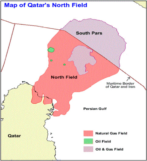
FIGURE 7. Schematic of Qatar’s North field.
Out of the 6067 data sets, the 2929 dataset related to well #W1 at a depth of 3700–4286 with a 0.2 m interval section is used, and the 1527 dataset related to well #W2 at a depth of 3649–3954 with a 0.2 m interval section, while the 1511 dataset related to well #W3 at a depth of 3772–4094 with a 0.2 m interval section is used. The data collected initially included spectral gamma ray (SGR); sonic porosity (PHIS); potassium (POTA); hole size (HS); caliper (BS); photoelectric absorption factor (PEF); neutron porosity (NPHI); sonic transition time (DT); bulk density (RHOB); corrected gamma ray (CGR); uranium (URAN) and thorium (THOR).
The feature selection method was used in order to remove unnecessary inputs and filter the data. Information about input variables and their related labels is presented in Table 3 and Figure 8. According to the feature selection method used in this article, as well as the reports in Table 4, it is determined that the first reports are taken for one category and the lowest RMSE value is reported for them, as well as for categories two, three, and... up to twelve. Finally, after reporting the best and lowest RMSE value for each category, we finally present the best report for the combination of inputs (which is 8 inputs here). The presented feature selection results are shown in Table 4. Feature selection results show that S1, S10, S6, S7, S9, S2, S8, S3 (SGR, PHIS, POTA, PEF, NPHI, DT, RHOB, CGR) show the best combination for FDVC prediction. After feature selection, the statical parameters of each well #W1, #W2 and #W3 and all wells of gas reservoirs located in Southwest Asia are shown in Tables 5, 6, respectively. The correlations between the input variables and output are explained further below. SGR is a measure of the radioactivity in the formation that is used for the determination of shale volume. Field practices show that in the fractured zone of formations presents a high GR value, due to the radioactive salts deposited on the fracture surface or inside the crack. A potassium log represents a continuous measure of the radioactive element potassium. Similarly, the presence of potassium salts deposited on the surface of fractures or inside the cracks in fractured formations causes a high potassium value. CGR log is similar to SGR log, except that CGR only accounts for thorium and potassium elements emitted by formation rock. As a result, it is expected that CGR log will behave similarly to SGR log in fractured formations. Bulk density is a log that represents the continuous measure of the bulk density of the formation. This log is applied for measuring the total porosity of reservoir formation. As a result of the filled-with-fluid fractures, the bulk density log decreases, as evidenced by a negative peak on the bulk density log. Neutron log provides a continuous record of the total porosity of reservoir formation, so it behaves similarly to the bulk density log in fractured zones. Sonic log is also a porosity log measures the travel time (DT) of acoustic waves through the formation. The time it takes for acoustic waves to travel through a unit length of rock is recorded in the DT log. As a result, the velocity of acoustic waves is expected to be low in fractures filled with fluid, and as a result, the DT log and sonic porosity logs are both expected to be high (Serra, 1983; Asquith et al., 2004; Haghighi, 2007; Taherdangkoo and Abdideh, 2016).
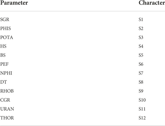
TABLE 3. Feature selection’s lable for input variables.
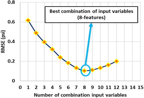
FIGURE 8. Determination of number of combination input variable for feature selection in well #W1.
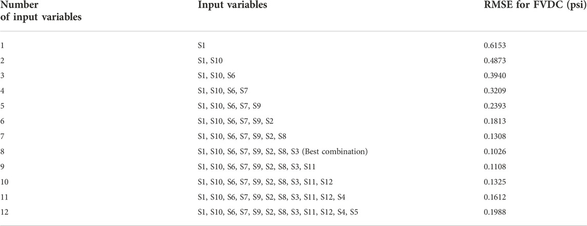
TABLE 4. Feature selection’s result to number of combination input variable for well #W1.
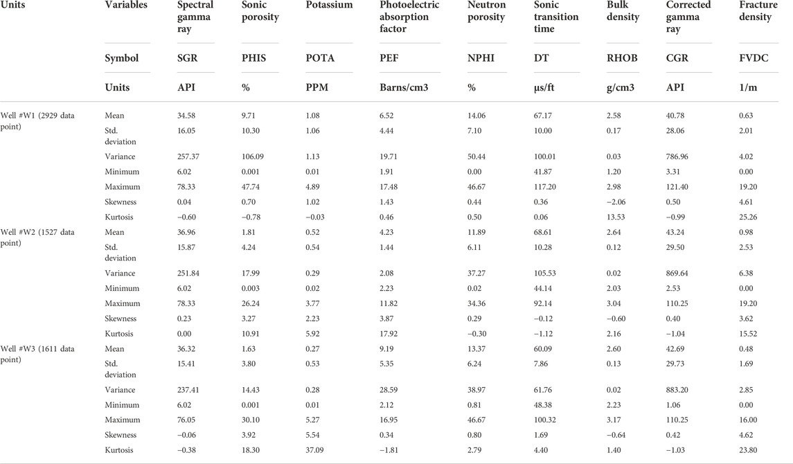
TABLE 5. Determination of statical parameter to prediction of FVDC of three wells of gas reservoirs located of Southwest Asia for each well seperatly (#W1, #W2 and #W3).
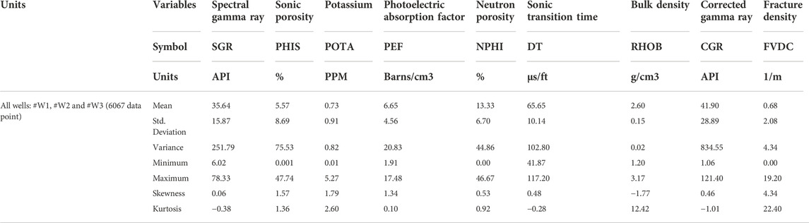
TABLE 6. Determination of statical parameter to prediction of FVDC for all three wells of gas reservoirs located of Southwest Asia (#W1, #W2 and #W3).
One of the functions that can interpret data and is very efficient is the cumulative distribution (CDF) functions, which can be used for any of the input and output variables (shown in Eq. 5). Figures 7, 8 show the interpretation of input and output variables for FVDC prediction. The information in these two forms is interpreted as follows (Abad et al., 2021a; Barjouei et al., 2021; Hazbeh et al., 2021):
where; εX (x) = The cumulative distribution functions; x = point for each input/output variable; X = the specific point data for each input/output variable x; and R = all data records for each input/output variable.
The schematic of Figure 9 shows the CFD diagram for four input variables datasets that include spectral gamma ray (SGR); sonic porosity (PHIS); potassium (POTA); photoelectric absorption factor (PEF).
• The value of CFD, for spectral gamma ray is SGR < 22.5 API for about 20% of the all-data record, 22.5 < SGR < 50 API for about 62% of the all-data record, and SGR > 50 API for about 18% of the all-data record.
• The value of CFD, for potassium is POTA < 0.1250 PPM for about 25.8% of the all-data record, 0.1250 < POTA < 1.56 PPM for about 60.6% of the all-data record, and POTA > 1.56 PPM for about 13.6% of the all-data record.
• The value of CFD, for sonic porosity is PHIS < 0.1059% for about 26% of the all-data record, 0.1059% < PHIS < 13.8%for about 56% of the all-data record, and PHIS > 13.8% for about 18% of the all-data record.
• The value of CFD, for photoelectric absorption factor is PEF < 3.9 Barn/cm3 for about 20% of the all-data record, 3.9 < PEF < 11.5 Barn/cm3 for about 53% of the all-data record, and PEF > 11.5 Barn/cm3 for about 3% of the all-data record.
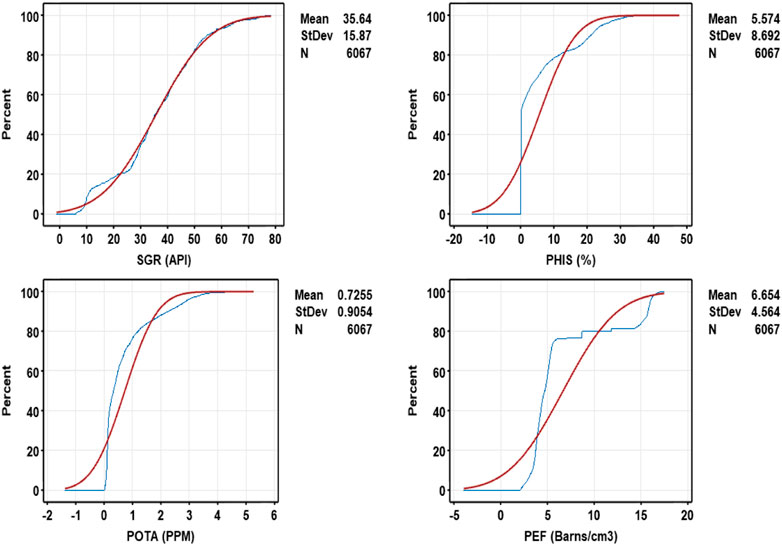
FIGURE 9. Schematic of the cumulative distribution function (CDF) to description four input variables dataset. The variable is: SGR; PHIS; POTA; PEF. In this figure, the blue and red line an input variable and standard deviation respectively.
Based on Figure 9, the variables SGR and POTA are almost normally distributed, whereas the variables PHIS and PEF do not conform to normal distributions.
Figure 10 depicts a CFD diagram for a dataset with five input/output variables: neutron porosity (NPHI), sonic transition time (DT), bulk density (RHOB), corrected gamma ray (CGR), and fracture density (FVDC).
• The value of CFD, for spectral gamma ray is NPHI < 13% for about 46% of the all-data record, 13 < NPHI < 22.4% for about 45% of the all-data record, and NPHI > 22.4% for about 9% of the all-data record.
• The value of CFD, for sonic porosity is DT < 68.5 μs/ft for about 13% of the all-data record, 54 < DT < 68.5 μs/ft for about 50% of the all-data record, and DT > 68.5 μs/ft for about 37% of the all-data record.
• The value of CFD, for potassium is RHOB < 2.65 g/cm3 for about 64% of the all-data record, 2.65 < RHOB < 2.8 g/cm3 for about 33% of the all-data record. and RHOB > 2.8 g/cm3 for about 3% of the all-data record.
• The value of CFD, for photoelectric absorption factor is CGR < 9.9 API for about 12% of the all-data record, 9.9 < CGR < 50 API for about 51% of the all-data record, and CGR > 50 API for about 37% of the all-data record.
• The value of CFD, for fracture density is FVDC < 0.15 1/m for about 40% of the all-data record, 0.15 < FVDC < 4 1/m for about 54% of the all-data record, and FVDC > 4 1/m for about 5% of the all-data record.
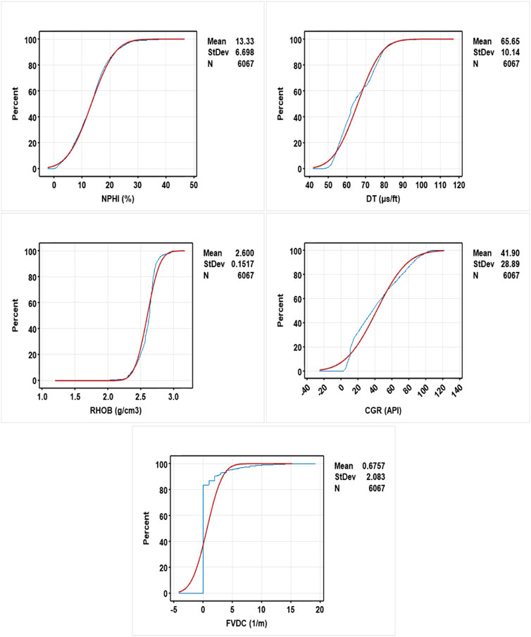
FIGURE 10. Schematic of the cumulative distribution function (CDF) to description five input/output variables dataset. The variable is: NPHI; DT; RHOB; CGR and FVDC. In this figure, the blue and red line an input variable and standard deviation respectively.
Based on Figure 10, the variable NPHI, DT and RHOB are almost normally distributed, whereas variables CGR and FVDC do not conform to normal distributions.
Result and discussion
One of the most important criteria used to compare the results of FVDC prediction using four hybrid artificial intelligence algorithms, LSSVM-PSO/GA and MLP-PSO/GA is the use of the following statistical indicators (Eqs 7–13) (Choubin et al., 2019; Shamshirband et al., 2020).
Percentage error (PE):
Mean relative error (MRE):
Mean absolute relative error (MARE):
Standard Deviation (STD):
Mean Square Error (MSE):
Root Mean Square Error (RMSE):
Coefficient of Determination (R2):
In order to develop hybrid machine learning robustness (LSSVM-PSO/GA and MLP-PSO/GA), information about well #W1 (2929 dataset) was used to predict FVDC. In this way, 70% of the 2929 data set (2049 subset) was used for training and construction and development of these algorithms, and 30% of the 2929 data set (880 subset) was used to test the results related to the algorithms. The train, test, and total results for each algorithm are shown in Table 7. The two most important parameters for determining and distinguishing the best artificial intelligence algorithms are the values of RMSE and R2 (Nabipour et al., 2020b; Farsi et al., 2021), which are discussed in detail.
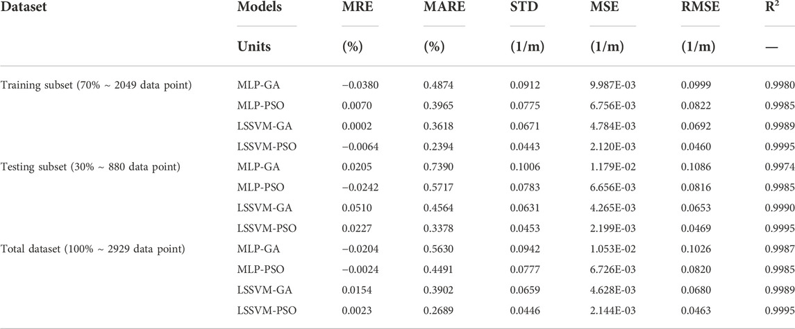
TABLE 7. Prediction of FVDC prediction performance for training, testing and total dataset based on four robust hybrid machine learning LSSVM-PSO, LSSVM-GA, MLP-PSO and MLP-GA based on dataset of well #W1.
The statistical error results in Table 7 shows that each of the four robust hybrid machine learning algorithms (LSSVM-PSO, LSSVM-GA, MLP-PSO, and MLP-GA) provides a more reliable prediction. After reviewing the results, it has been determined that the highest performance accuracy is related to the LSSVM-PSO algorithm. The error value according to Table 7, the MELM-PSO model has: RMSE = 0.0460 1/m; MARE = 0.2394 ٪; R2 = 0.9996 for training subset; RMSE = 0.0469 1/ m; MARE = 0.3378 ٪; R2 = 0.9996 for testing subset; and RMSE = 0.0463 1/ m; MARE = 0.2689 ٪; R2 = 0.9995 for total subset.
Figures 11–13 shows the illustration of the cross plot for training, testing, and total subset based on four robust hybrid machine learning algorithms: LSSVM-PSO, LSSVM-GA, MLP-PSO, and MLP-GA based on the dataset of well #W1. In the first place, these graphs show an eye scan for the accuracy of the operation of each algorithm, and in the second place, they show the correlation coefficient for the predicted points versus the measured points against the tradeline line. After examining the diagram, it is found that the performance accuracy of the algorithms for predicting FVDC includes LSSVM-PSO> LSSVM-GA> MLP-PSO> MLP-GA, respectively.
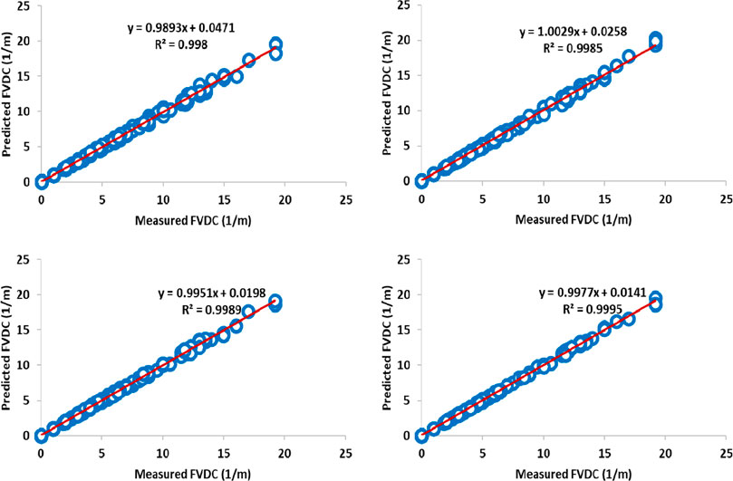
FIGURE 11. llustration of cross plot for training subset (70% ∼ 2049 data point) based on four roboust hybrid machine learning LSSVM-PSO, LSSVM-GA, MLP-PSO and MLP-GA based on dataset of well #W1.
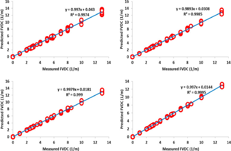
FIGURE 12. llustration of cross plot for training subset (70% ∼ 2049 data point) based on four roboust hybrid machine learning LSSVM-PSO, LSSVM-GA, MLP-PSO and MLP-GA based on dataset of well #W1.
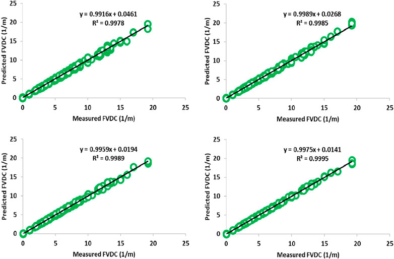
FIGURE 13. llustration of cross plot for training subset (70% ∼ 2049 data point) based on four roboust hybrid machine learning LSSVM-PSO, LSSVM-GA, MLP-PSO and MLP-GA based on dataset of well #W1.
Figure 14 shows the histogram for the prediction error value of FVDC for the four AI-based hybrid robust based on the dataset of well #W1. As shown in this figure, the normal error distribution for the LSSVM-PSO model is not better than for other models. In addition, as it is clear, the MELM-PSO error range is much less than other models. The ratio is lower than for other models, indicating that this robust artificial intelligence hybrid model outperforms other models in terms of performance accuracy.
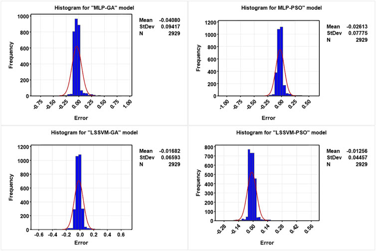
FIGURE 14. Fracture density’s (FVDC) histogram and distribution line for determination of highly accuracy for four roboust hybrid machine learning LSSVM-PSO, LSSVM-GA, MLP-PSO and MLP-GA based on dataset of well #W1.
Figure 15 shows the RMSE value per iteration. Based on this figure, it is determined that the convergence speed of all four robust hybrid machine learning algorithms is the same, and all four algorithms converge at iteration = 4 and continue with the same convergence speed. At the end of this step (iteration = 200) as it was clear at the beginning (iteration = 4), the accuracy of the algorithms is LSSVM-PSO> LSSVM-GA> MLP-PSO> MLP-GA, respectively.
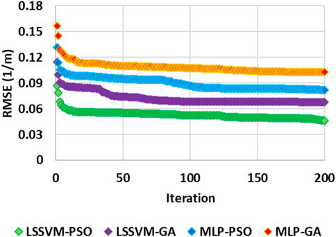
FIGURE 15. The RMSE vs. iteration for determination of the for four roboust hybrid machine learning LSSVM-PSO, LSSVM-GA, MLP-PSO and MLP-GA based on dataset of well #W1.
Generalization of new robust Least-squares support-vector machines-particle swarm optimizer algorithm to predicted fracture density
After reviewing the results of the four applied robust artificial intelligence hybrid algorithms (LSSVM-PSO, LSSVM-GA, MLP-PSO, and MLP-GA) using well information from well #W1, it was found that the LSSVM-PSO algorithm has higher performance accuracy than other algorithms (i.e., LSSVM-GA, MLP-PSO and MLP-GA). To develop and generalize the best artificial intelligence algorithm for FVDC prediction, this robust algorithm predicted with information from two other wells (#W2 and #W3). The results presented in Table 8 and the results presented in Figures 16, 17 demonstarte the high-performance accuracy of this algorithm. It is also suggested that the developed algorithm be applied to other important reservoir engineering parameters.
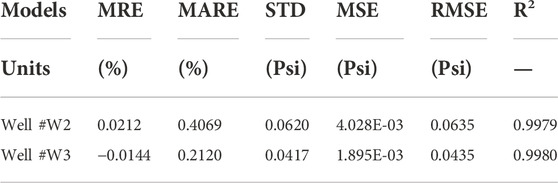
TABLE 8. Development and generalization of new robust hybrid machine learning LSSVM-PSO algorithm that structured by training subset of well #W1 for prediction FVDC related to wells #W2 and #W3.
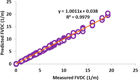
FIGURE 16. llustration of cross plot of new robust LSSVM-PSO algorithm structered by training subset of well #W1 for prediction FVDC related to wells #W2.
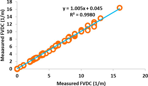
FIGURE 17. llustration of cross plot of new robust LSSVM-PSO algorithm structered by training subset of well #W1 for prediction FVDC related to wells #W2.
Conclusion and recommendation
The datasets of three wells from a gas reservoirs located in Southwest Asia were analyzed to predict the fracture density using petrophysical log data. The input variables were filtered using the feature selection method, and the following input variables were used in this paper: spectral gamma ray (SGR); sonic porosity (PHIS); potassium (POTA); photoelectric absorption factor (PEF); neutron porosity (NPHI); sonic transition time (DT); bulk density (RHOB); and corrected gamma ray (CGR). To predict this important parameter, four hybrid algorithms (LSSVM-PSO/GA and MLP-PSO/GA) have been used. In order to build hybrid algorithms, 2929 datasets related to #W1 data were used to build and develop hybrid algorithms (training = 2049 subset, testing = 880 subset). After reviewing the results and comparing algorithms using statical parameters, it was determined that the performance accuracy of algorithms for FVDC prediction is LSSVM-PSO> LSSVM-GA> MLP-PSO> MLP-GA. LSSVM-PSO is the best algorithm for predicting FVDC among the four algorithms (RMSE = 0.0463 1/m; R2 = 0.9995). This algorithm has several advantages, including: 1) lower adjustment parameters, 2) high search efficiency, 3) fast convergence speed, 4) increased global search capability, and 5) prevention of fall in the local optimum. A comparison of this model to other models reveals that it has a significantly lower error than other algorithms, and after investigating other wells in this field, it was discovered that the generalizability of this algorithm is very suitable and can be used to predict FVDC for other gas fields. It is strongly recommended that this algorithm be used when high speed and accuracy are required, as well as when the noise level of numbers is low. In addition, the k-fold cross validation method with k equal to 8 was used in this article. Researchers can predict the amount of empty space in the rock (existing fractures) by comparing the flow in the porous medium and studying the flow to determine the amount of rock fractures. The following key points can be considered in future works:
1) Applying the predicted fracture density as input for flow simulation, which can further confirm the validation of the predictions made by the hybrid models developed and is undoubtedly useful in modeling flow in fractured reservoirs.
2) Test and evaluate the hybrid models developed for fracture density prediction on new datasets from another field to provide valuable insight on their generalizability.
Data availability statement
Data can be made available upon reasonable requests for academic purposes through the corresponding authors.
Author contributions
Conceptualization, HG, AM, MC, OH, and GG; methodology, SD, MR, GG, and HG; software, AM and HG; validation, HG, MC, GG, and SD; formal analysis, MR, GG and HG; investigation, ST, MC, GG, AM, and HG; resources, OH, ST, GG, and HG; data curation, AM and HG; writing—original draft preparation, SD, GG, MR, HG, AR, and ST; writing—review and editing, AR, GG, HG, and MC; visualization, MR, GG, ST, HG, and AR; supervision, HG, MC, and AM; project administration, HG, GG, and AM. All authors have read and agreed to the published version of the manuscript.
Funding
This research was supported by the Tomsk Polytechnic University development program. And also, this work was supported by the Open Foundation of Cooperative Innovation Center of Unconventional Oil and Gas, Yangtze University (Ministry of Education & Hubei Province), No. UOG 2022-05.
Conflict of interest
The authors declare that the research was conducted in the absence of any commercial or financial relationships that could be construed as a potential conflict of interest.
Publisher’s note
All claims expressed in this article are solely those of the authors and do not necessarily represent those of their affiliated organizations, or those of the publisher, the editors and the reviewers. Any product that may be evaluated in this article, or claim that may be made by its manufacturer, is not guaranteed or endorsed by the publisher.
References
Abad, A. R. B., Mousavi, S., Mohamadian, N., Wood, D. A., Ghorbani, H., Davoodi, S., et al. (2021a). Hybrid machine learning algorithms to predict condensate viscosity in the near wellbore regions of gas condensate reservoirs. J. Nat. Gas Sci. Eng. 95, 104210. doi:10.1016/j.jngse.2021.104210
Abad, A. R. B., Tehrani, P. S., Naveshki, M., Ghorbani, H., Mohamadian, N., Davoodi, S., et al. (2021b). Predicting oil flow rate through orifice plate with robust machine learning algorithms. Flow Meas. Instrum. 81, 102047. doi:10.1016/j.flowmeasinst.2021.102047
Abad, A. R. B., Ghorbani, H., Mohamadian, N., Davoodi, S., Mehrad, M., Aghdam, S. K.-Y., et al. (2022). Robust hybrid machine learning algorithms for gas flow rates prediction through wellhead chokes in gas condensate fields. Fuel 308, 121872. doi:10.1016/j.fuel.2021.121872
Ahmadi, M. H., Baghban, A., Sadeghzadeh, M., Zamen, M., Mosavi, A., Shamshirband, S., et al. (2020). Evaluation of electrical efficiency of photovoltaic thermal solar collector. Eng. Appl. Comput. Fluid Mech. 14, 545–565. doi:10.1080/19942060.2020.1734094
Ali, F. F., Hamoudi, M. R., and Wahab, A. H. A. (2021). Analyzing the factors contributing to water coning in a naturally fractured oil reservoir of Kurdistan Region of Iraq. IEEE, 172–177.
Ashrafi, S. B., Anemangely, M., Sabah, M., and Ameri, M. J. (2019). Application of hybrid artificial neural networks for predicting rate of penetration (rop): A case study from Marun oil field. J. petroleum Sci. Eng. 175, 604–623. doi:10.1016/j.petrol.2018.12.013
Asquith, G. B., Krygowski, D., and Gibson, C. R. (2004). Basic well log analysis. American Association of Petroleum Geologists Tulsa.
Band, S. S., Janizadeh, S., Chandra Pal, S., Saha, A., Chakrabortty, R., Melesse, A. M., et al. (2020). Flash flood susceptibility modeling using new approaches of hybrid and ensemble tree-based machine learning algorithms. Remote Sens. 12, 3568. doi:10.3390/rs12213568
Barjouei, H. S., Ghorbani, H., Mohamadian, N., Wood, D. A., Davoodi, S., Moghadasi, J., et al. (2021). Prediction performance advantages of deep machine learning algorithms for two-phase flow rates through wellhead chokes. J. Pet. Explor. Prod. Technol. 11, 1233–1261. doi:10.1007/s13202-021-01087-4
Beheshtian, S., Rajabi, M., Davoodi, S., Wood, D. A., Ghorbani, H., Mohamadian, N., et al. (2022). Robust computational approach to determine the safe mud weight window using well-log data from a large gas reservoir. Mar. Petroleum Geol. 142, 105772. doi:10.1016/j.marpetgeo.2022.105772
Bessa, F., Jerath, K., Ginn, C., Johnston, P., Zhao, Y., Brown, T., et al. (2021). Subsurface characterization of hydraulic fracture test site-2 (HFTS-2), Delaware basin. Houston, TX: OnePetro.
Bhattacharya, S., and Mishra, S. (2018). Applications of machine learning for facies and fracture prediction using Bayesian Network Theory and Random Forest: Case studies from the Appalachian basin, USA. J. Petrol. Sci. Eng. 170, 1005–1017.
Chandrashekar, G., and Sahin, F. (2014). A survey on feature selection methods. Comput. Electr. Eng. 40, 16–28. doi:10.1016/j.compeleceng.2013.11.024
Choubin, B., Mosavi, A., Alamdarloo, E. H., Hosseini, F. S., Shamshirband, S., Dashtekian, K., et al. (2019). Earth fissure hazard prediction using machine learning models. Environ. Res. 179, 108770. doi:10.1016/j.envres.2019.108770
Cortes, C., and Vapnik, V. (1995). Support-vector networks. Mach. Learn. 20, 273–297. doi:10.1007/bf00994018
Faraji, F., Santim, C., Chong, P. L., and Hamad, F. (2022). Two-phase flow pressure drop modelling in horizontal pipes with different diameters. Nucl. Eng. Des. 395, 111863. doi:10.1016/j.nucengdes.2022.111863
Farsi, M., Mohamadian, N., Ghorbani, H., Wood, D. A., Davoodi, S., Moghadasi, J., et al. (2021). Predicting formation pore-pressure from well-log data with hybrid machine-learning optimization algorithms. Nat. Resour. Res. 30, 3455–3481. doi:10.1007/s11053-021-09852-2
Ghalandari, M., Ziamolki, A., Mosavi, A., Shamshirband, S., Chau, K.-W., and Bornassi, S. (2019). Aeromechanical optimization of first row compressor test stand blades using a hybrid machine learning model of genetic algorithm, artificial neural networks and design of experiments. Eng. Appl. Comput. Fluid Mech. 13, 892–904. doi:10.1080/19942060.2019.1649196
Gholami, R., and Fakhari, N. (2017). “Support vector machine: Principles, parameters, and applications,” in Handbook of neural computation (Elsevier), 515–535.
Ghorbani, H., Wood, D. A., Mohamadian, N., Rashidi, S., Davoodi, S., Soleimanian, A., et al. (2020). Adaptive neuro-fuzzy algorithm applied to predict and control multi-phase flow rates through wellhead chokes. Flow Meas. Instrum. 76, 101849. doi:10.1016/j.flowmeasinst.2020.101849
Ghorbani, H., Davoodi, S., and Davarpanah, A. (2021). Accurate determination of shear wave velocity using LSSVM-GA algorithm based on petrophysical log. Larnaca, Cyprus: European Association of Geoscientists & Engineers, 1–3.
H Ghorbani, S. D., and Davarpanah, A. (2021). “Accurate determination of shear wave velocity using LSSVM-GA algorithm based on petrophysical log,” in Third EAGE eastern mediterranean workshop, 1–3.
Haghighi, M. (2007). “Using conventional logs for fracture detection and characterization in one of Iranian field,” in International petroleum technology conference.
Hashemizadeh, A., Bahonar, E., Chahardowli, M., Kheirollahi, H., and Simjoo, M. (2022). A data-driven approach to estimate the rate of penetration in drilling of hydrocarbon reservoirs.
Hassanat, A., Almohammadi, K., Alkafaween, E., Abunawas, E., Hammouri, A., and Prasath, V. (2019). Choosing mutation and crossover ratios for genetic algorithms—A review with a new dynamic approach. Information 10, 390. doi:10.3390/info10120390
Hassanpouryouzband, A., Joonaki, E., Edlmann, K., Heinemann, N., and Yang, J. (2020). Thermodynamic and transport properties of hydrogen containing streams. Sci. Data 7 (1), 1–14. doi:10.1038/s41597-020-0568-6
Hassanpouryouzband, A., Joonaki, E., Edlmann, K., and Haszeldine, R. S. (2021). Offshore geological storage of hydrogen: Is this our best option to achieve net-zero? ACS Energy Lett. 6, 2181–2186. doi:10.1021/acsenergylett.1c00845
Hassanpouryouzband, A., Adie, K., Cowen, T., Thaysen, E. M., Heinemann, N., Butler, I. B., et al. (2022). Geological hydrogen storage: Geochemical reactivity of hydrogen with sandstone reservoirs. ACS Energy Lett. 7, 2203–2210. doi:10.1021/acsenergylett.2c01024
Hazbeh, O., Aghdam, S. K.-Y., Ghorbani, H., Mohamadian, N., Alvar, M. A., and Moghadasi, J. (2021). Comparison of accuracy and computational performance between the machine learning algorithms for rate of penetration in directional drilling well. Petroleum Res. 6, 271–282. doi:10.1016/j.ptlrs.2021.02.004
Holland, J. H. (1984). “Genetic algorithms and adaptation,” in Adaptive control of ill-defined systems (Springer), 317–333.
Ibrahim, A. F., Elkatatny, S., Abdelraouf, Y., and Al Ramadan, M. (2022). Application of various machine learning techniques in predicting water saturation in tight gas sandstone formation. J. Energy Resour. Technol. 144, 083009. doi:10.1115/1.4053248
Ince, R. (2004). Prediction of fracture parameters of concrete by artificial neural networks. Eng. Fract. Mech. 71, 2143–2159. doi:10.1016/j.engfracmech.2003.12.004
Ja'fari, A., Kadkhodaie-Ilkhchi, A., Sharghi, Y., and Ghanavati, K. (2012). Fracture density estimation from petrophysical log data using the adaptive neuro-fuzzy inference system. J. Geophys. Eng. 9, 105–114. doi:10.1088/1742-2132/9/1/013
Jafarizadeh, F., Rajabi, M., Tabasi, S., Seyedkamali, R., Davoodi, S., Ghorbani, H., et al. (2022). Data driven models to predict pore pressure using drilling and petrophysical data. Energy Rep. 8, 6551–6562. doi:10.1016/j.egyr.2022.04.073
Jain, A., and Zongker, D. (1997). Feature selection: Evaluation, application, and small sample performance. IEEE Trans. Pattern Anal. Mach. Intell. 19, 153–158. doi:10.1109/34.574797
Kamali, M. Z., Davoodi, S., Ghorbani, H., Wood, D. A., Mohamadian, N., Lajmorak, S., et al. (2022). Permeability prediction of heterogeneous carbonate gas condensate reservoirs applying group method of data handling. Mar. Petroleum Geol. 139, 105597. doi:10.1016/j.marpetgeo.2022.105597
Kıran, M. S., Özceylan, E., Gündüz, M., and Paksoy, T. (2012). A novel hybrid approach based on particle swarm optimization and ant colony algorithm to forecast energy demand of Turkey. Energy Convers. Manag. 53, 75–83. doi:10.1016/j.enconman.2011.08.004
Kuo, R., Hong, S., and Huang, Y. (2010). Integration of particle swarm optimization-based fuzzy neural network and artificial neural network for supplier selection. Appl. Math. Model. 34, 3976–3990. doi:10.1016/j.apm.2010.03.033
Lai, J., Wang, G., Fan, Z., Chen, J., Qin, Z., Xiao, C., et al. (2017). Three-dimensional quantitative fracture analysis of tight gas sandstones using industrial computed tomography. Sci. Rep. 7 (1), 1–12. doi:10.1038/s41598-017-01996-7
Madani, M., Moraveji, M. K., and Sharifi, M. (2021). Modeling apparent viscosity of waxy crude oils doped with polymeric wax inhibitors. J. Petroleum Sci. Eng. 196, 108076. doi:10.1016/j.petrol.2020.108076
Mahdaviara, M., Menad, N. A., Ghazanfari, M. H., and Hemmati-Sarapardeh, A. (2020). Modeling relative permeability of gas condensate reservoirs: Advanced computational frameworks. J. Petroleum Sci. Eng. 189, 106929. doi:10.1016/j.petrol.2020.106929
Mahendran, N., and Durai Raj, V. P. (2021). A deep learning framework with an embedded-based feature selection approach for the early detection of the Alzheimer's disease. Comput. Biol. Med. 141, 105056. doi:10.1016/j.compbiomed.2021.105056
Miah, M. I. (2021). Improved prediction of shear wave velocity for clastic sedimentary rocks using hybrid model with core data. J. Rock Mech. Geotechnical Eng. 13, 1466–1477. doi:10.1016/j.jrmge.2021.06.014
Mirzaei-Paiaman, A., and Salavati, S. (2012). The application of artificial neural networks for the prediction of oil production flow rate. Energy Sources, Part A Recovery, Util. Environ. Eff. 34, 1834–1843. doi:10.1080/15567036.2010.492386
Mohamadian, N., Ghorbani, H., Wood, D. A., Mehrad, M., Davoodi, S., Rashidi, S., et al. (2021). A geomechanical approach to casing collapse prediction in oil and gas wells aided by machine learning. J. Petroleum Sci. Eng. 196, 107811. doi:10.1016/j.petrol.2020.107811
Mosavi, A., Faghan, Y., Ghamisi, P., Duan, P., Ardabili, S. F., Salwana, E., et al. (2020). Comprehensive review of deep reinforcement learning methods and applications in economics. Mathematics 8, 1640. doi:10.3390/math8101640
Nabipour, M., Nayyeri, P., Jabani, H., Shahab, S., and Mosavi, A. (2020a). Predicting stock market trends using machine learning and deep learning algorithms via continuous and binary data; a comparative analysis. IEEE Access 8, 150199–150212. doi:10.1109/access.2020.3015966
Nabipour, N., Mosavi, A., Hajnal, E., Nadai, L., Shamshirband, S., and Chau, K.-W. (2020b). Modeling climate change impact on wind power resources using adaptive neuro-fuzzy inference system. Eng. Appl. Comput. Fluid Mech. 14, 491–506. doi:10.1080/19942060.2020.1722241
Nawi, N. M., Rehman, M., Aziz, M. A., Herawan, T., and Abawajy, J. H. (2014). “An accelerated particle swarm optimization based Levenberg Marquardt back propagation algorithm,” in International conference on neural information processing (Springer), 245–253.
Nourani, M., Alali, N., Samadianfard, S., Band, S. S., Chau, K.-W., and Shu, C.-M. (2022). Comparison of machine learning techniques for predicting porosity of chalk. J. Petroleum Sci. Eng. 209, 109853. doi:10.1016/j.petrol.2021.109853
Nouri-Taleghani, M., Mahmoudifar, M., Shokrollahi, A., Tatar, A., and Karimi-Khaledi, M. (2015). Fracture density determination using a novel hybrid computational scheme: A case study on an Iranian Marun oil field reservoir. J. Geophys. Eng. 12, 188–198. doi:10.1088/1742-2132/12/2/188
Pang, H., Meng, H., Wang, H., Fan, Y., Nie, Z., and Jin, Y. (2022). Lost circulation prediction based on machine learning. J. Petroleum Sci. Eng. 208, 109364. doi:10.1016/j.petrol.2021.109364
Qasem, S. N., Samadianfard, S., Sadri Nahand, H., Mosavi, A., Shamshirband, S., and Chau, K.-W. (2019). Estimating daily dew point temperature using machine learning algorithms. Water 11, 582. doi:10.3390/w11030582
Radwan, A. E., Nabawy, B. S., Kassem, A. A., and Hussein, W. S. (2021). Implementation of rock typing on waterflooding process during secondary recovery in oil reservoirs: A case study, el morgan oil field, gulf of suez, Egypt. Nat. Resour. Res. 30, 1667–1696. doi:10.1007/s11053-020-09806-0
Rady, E.-H. A., and Anwar, A. S. (2019). Prediction of kidney disease stages using data mining algorithms. Inf. Med. Unlocked 15, 100178. doi:10.1016/j.imu.2019.100178
Rajabi, M., Beheshtian, S., Davoodi, S., Ghorbani, H., Mohamadian, N., Radwan, A. E., et al. (2021). Novel hybrid machine learning optimizer algorithms to prediction of fracture density by petrophysical data. J. Pet. Explor. Prod. Technol. 11, 4375–4397. doi:10.1007/s13202-021-01321-z
Rajabi, M., Ghorbani, H., and Aghdam, K.-Y. (2022a). Prediction of shear wave velocity by extreme learning machine technique from well log data. J. Petroleum Geomechanics 4, 18–35. doi:10.22107/JPG.2022.298520.1151
Rajabi, M., Ghorbani, H., and Aghdam, K.-Y. (2022b). Sensitivity analysis of effective factors for estimating formation pore pressure using a new method: The LSSVM-PSO algorithm. J. Petroleum Geomechanics 4, 19–39. doi:10.22107/JPG.2022.298551.1152
Rajabi, M., Ghorbani, H., and Lajmorak, S. (2022c). Comparison of artificial intelligence algorithms to predict pore pressure using petrophysical log data. J. Struct. Constr. Eng. doi:10.22065/JSCE.2022.309523.2600
Rajabi, M., Hazbeh, O., Davoodi, S., Wood, D. A., Tehrani, P. S., Ghorbani, H., et al. (2022d). Predicting shear wave velocity from conventional well logs with deep and hybrid machine learning algorithms. J. Pet. Explor. Prod. Technol., 1–24. doi:10.1007/s13202-022-01531-z
Rashidi, S., Mehrad, M., Ghorbani, H., Wood, D. A., Mohamadian, N., Moghadasi, J., et al. (2021). Determination of bubble point pressure & oil formation volume factor of crude oils applying multiple hidden layers extreme learning machine algorithms. J. Petroleum Sci. Eng. 202, 108425. doi:10.1016/j.petrol.2021.108425
Roffo, G., Melzi, S., Castellani, U., Vinciarelli, A., and Cristani, M. (2020). Infinite feature selection: A graph-based feature filtering approach. IEEE Trans. Pattern Anal. Mach. Intell. 43, 4396–4410. doi:10.1109/tpami.2020.3002843
Sadeghnejad, S., Ashrafizadeh, M., and Nourani, M. (2022). “Improved oil recovery by gel technology: Water shutoff and conformance control,” in Chemical methods (Elsevier), 249–312.
Shabani, S., Samadianfard, S., Sattari, M. T., Mosavi, A., Shamshirband, S., Kmet, T., et al. (2020). Modeling pan evaporation using Gaussian process regression K-nearest neighbors random forest and support vector machines; comparative analysis. Atmosphere 11, 66. doi:10.3390/atmos11010066
Shamshirband, S., Mosavi, A., Rabczuk, T., Nabipour, N., and Chau, K.-W. (2020). Prediction of significant wave height; comparison between nested grid numerical model, and machine learning models of artificial neural networks, extreme learning and support vector machines. Eng. Appl. Comput. Fluid Mech. 14, 805–817. doi:10.1080/19942060.2020.1773932
Sipahi, M. T., and Develi, K. (2021). Modelling of hydraulic fracturing treatments in south east part of Turkey with dfn method and comparison with simulation results. OnePetro.
Sivanandam, S., and Deepa, S. (2008). “Genetic algorithms,” in Introduction to genetic algorithms (Springer), 15–37.
Soares, C., and Gray, K. (2019). Real-time predictive capabilities of analytical and machine learning rate of penetration (ROP) models. J. Petroleum Sci. Eng. 172, 934–959. doi:10.1016/j.petrol.2018.08.083
Suykens, J. A., Van Gestel, T., De Brabanter, J., De Moor, B., and Vandewalle, J. P. (2002). Least squares support vector machines. World Scientific.
Suykens, J. A., and Vandewalle, J. (1999). Least squares support vector machine classifiers. Neural Process. Lett. 9, 293–300. doi:10.1023/a:1018628609742
Syah, R., Ahmadian, N., Elveny, M., Alizadeh, S., Hosseini, M., and Khan, A. (2021). Implementation of artificial intelligence and support vector machine learning to estimate the drilling fluid density in high-pressure high-temperature wells. Energy Rep. 7, 4106–4113. doi:10.1016/j.egyr.2021.06.092
Tabasi, S., Tehrani, P. S., Rajabi, M., Wood, D. A., Davoodi, S., Ghorbani, H., et al. (2022). Optimized machine learning models for natural fractures prediction using conventional well logs. Fuel 326, 124952. doi:10.1016/j.fuel.2022.124952
Taherdangkoo, R., and Abdideh, M. (2016). Fracture density estimation from well logs data using regression analysis: Validation based on image logs (case study: South west Iran). Int. J. Petroleum Eng. 2, 289–301. doi:10.1504/ijpe.2016.084117
Taherei Ghazvinei, P., Hassanpour Darvishi, H., Mosavi, A., Yusof, K. B. W., Alizamir, M., Shamshirband, S., et al. (2018). Sugarcane growth prediction based on meteorological parameters using extreme learning machine and artificial neural network. Eng. Appl. Comput. Fluid Mech. 12, 738–749. doi:10.1080/19942060.2018.1526119
Torabi, M., Hashemi, S., Saybani, M. R., Shamshirband, S., and Mosavi, A. (2019). A Hybrid clustering and classification technique for forecasting short-term energy consumption. Environ. Prog. Sustain. Energy 38, 66–76. doi:10.1002/ep.12934
Vera-Rozo, J. R., Sáez-Bastante, J., Carmona-Cabello, M., Riesco-Ávila, J. M., Avellaneda, F., Pinzi, S., et al. (2022). Cetane index prediction based on biodiesel distillation curve. Fuel 321, 124063. doi:10.1016/j.fuel.2022.124063
Wahab, M. N. A., Nefti-Meziani, S., and Atyabi, A. (2015). A comprehensive review of swarm optimization algorithms. PloS one 10, e0122827–e0122836. doi:10.1371/journal.pone.0122827
Yang, L. I., Zhijiang, K., Zhaojie, X. U. E., and Zheng, S. (2018). Theories and practices of carbonate reservoirs development in China. Petroleum Explor. Dev. 45, 712–722. doi:10.1016/s1876-3804(18)30074-0
Zazoun, R. S. (2013). Fracture density estimation from core and conventional well logs data using artificial neural networks: The Cambro-Ordovician reservoir of Mesdar oil field, Algeria. J. Afr. Earth Sci. 83, 55–73. doi:10.1016/j.jafrearsci.2013.03.003
Zhang, C., Zhang, T., and Yuan, C. (2011). Oil holdup prediction of oil–water two phase flow using thermal method based on multiwavelet transform and least squares support vector machine. Expert Syst. Appl. 38, 1602–1610. doi:10.1016/j.eswa.2010.07.081
Zhang, Z., Zhang, H., Li, J., and Cai, Z. (2021). Permeability and porosity prediction using logging data in a heterogeneous dolomite reservoir: An integrated approach. J. Nat. Gas Sci. Eng. 86, 103743. doi:10.1016/j.jngse.2020.103743
Zhang, G., Davoodi, S., Shamshirband, S., Ghorbani, H., Mosavi, A., and Moslehpour, M. (2022). A robust approach to pore pressure prediction applying petrophysical log data aided by machine learning techniques. Energy Rep. 8, 2233–2247. doi:10.1016/j.egyr.2022.01.012
Zheng, L., Wei, P., Zhang, Z., Nie, S., Lou, X., Cui, K., et al. (2017). Joint exploration and development: A self-salvation road to sustainable development of unconventional oil and gas resources. Nat. Gas. Ind. B 4, 477–490. doi:10.1016/j.ngib.2017.09.010
Nomenclature
ANN Artificial neural network
dmax Maximum aggregate size
w/c Water-cation ratio
fc Compressive strength
E Young’s modulus
DT Sonic transient time
ANFIS Adaptive neuro-fuzzy inference system
RHOB Bulk density
RT Deep resistance Deep resistivity
NPHI Neutron porosity
RT Deep resistance Deep resistivity
CIMS Committee machine intelligent system
FVDC Fracture density
HS Caliper Hole size
D Depth
PEF Photoelectric absorption factor
Qi The normalize value of data records i
Qmin The minimum value of each variable
Qmax The maximum value of each variable
SGR Spectral gamma ray
PHIS Sonic porosity
POTA Potassium
BS Caliper
L Length
n number of sample unit
URAN Uranium
CGR Corrected gamma ray
THOR Thorium
b Bias
C Cost Function
c1 Positive cognitive coefficient (individual learning factors PSO)
c2 Positive social coefficient (global learning factor for PSO)
GA Genetic algorithm
LS-SVM Least Squares Support Vector Machine
LM Levenberg-Marquardt
MLP Multi-Layer Perceptron
PSO Particle swarm optimization
RBF Radial basis function
RMSE Root means square error
SVM Support Vector Machines
T transpose matrix
Keywords: machine learning, least-squares support-vector machines, fracture density, prediction, artificial intelligence, energy, big data
Citation: Gao G, Hazbeh O, Davoodi S, Tabasi S, Rajabi M, Ghorbani H, Radwan AE, Csaba M and Mosavi AH (2023) Prediction of fracture density in a gas reservoir using robust computational approaches. Front. Earth Sci. 10:1023578. doi: 10.3389/feart.2022.1023578
Received: 19 August 2022; Accepted: 12 September 2022;
Published: 05 January 2023.
Edited by:
Muhsan Ehsan, Bahria University, PakistanReviewed by:
Aliakbar Hassanpouryouzband, University of Edinburgh, United KingdomKaveh Abbasi Kololi, Islamic Azad University, Bushehr, Iran
Copyright © 2023 Gao, Hazbeh, Davoodi, Tabasi, Rajabi, Ghorbani, Radwan, Csaba and Mosavi. This is an open-access article distributed under the terms of the Creative Commons Attribution License (CC BY). The use, distribution or reproduction in other forums is permitted, provided the original author(s) and the copyright owner(s) are credited and that the original publication in this journal is cited, in accordance with accepted academic practice. No use, distribution or reproduction is permitted which does not comply with these terms.
*Correspondence: Hamzeh Ghorbani, aGFtemVoZ2hvcmJhbmk2OEB5YWhvby5jb20=; Amir H. Mosavi, YW1pcmhvc2Vpbi5tb3NhdmlAc3R1YmEuc2s=