Quantitative estimation of sentinel-1A interferometric decorrelation using vegetation index

Sentinel-1A data are widely used in interferometric synthetic aperture radar (InSAR) studies due to the free and open access policy. However, the short wavelength (C-band) of Sentinal-1A data leads to decorrelation in numerous applications, especially in vegetated areas. Phase blurring and reduced monitoring accuracy can occur owing to changes in the physical and chemical characteristics of vegetation during the satellite revisit period, which essentially makes poor use of SAR data and increases the time and economic costs for researchers. Interferometric coherence is a commonly used index to measure the interference quality of two single-look complex (SLC) images, and its value can be used to characterize the decorrelation degree. The normalized difference vegetation index (NDVI) is obtained from optical images, and its value can be used to characterize the surface vegetation coverage. In order to solve the problem that Sentinel-1A decorrelation in the vegetated area is difficult to estimate prior to single-look complex interference, this paper selects a vegetated area in Sichuan Province, China as the study area and establishes two two-order linear quantitative models between Landsat8-derived normalized difference vegetation index and Sentinel-1A interferometric coherence in co- and cross-polarization: When NDVI at extremely high and low levels, coherence is close to zero, while NDVI and coherence show two different linear relationships in co- and cross-polarization in terms of NDVI at the middle level. The models global error basically obeys the normal distribution with the mean value of −0.037 and −0.045, and the standard deviation of 0.205 and 0.201 at the VV and VH channels. The two models are then validated in two validation areas, and the results confirm the reliability of the models and reveal the relationships between Sentinel-1A InSAR decorrelation and vegetation coverage in co- and cross-polarization, thus demonstrating that the NDVI can be applied to quantitatively estimate the InSAR decorrelation in vegetated area of Sentinel-1A data in both polarization modes prior to SLC interference.

1 Introduction

Sentinel-1A data were made available to users worldwide on 3 October 2014 (Potin et al., 2016). Since the time, Sentinel-1A data have been widely used in seismic and geological structure monitoring (Suresh and Yarrakula, 2020; Han et al., 2022), volcano monitoring (Guo et al., 2019; Bato et al., 2021; Corsa et al., 2022), glacier monitoring (Liang et al., 2021a; Zhang et al., 2021a; Manjula et al., 2022), agricultural monitoring and mapping (Diniz et al., 2022; Guo et al., 2022; Wuyun et al., 2022), other deformation mapping fields (Dai et al., 2016; He et al., 2020; Zhao et al., 2020), and are also an important C-band (wavelength = 5.5 cm) data source in the field of interferometric synthetic aperture radar (InSAR) and agriculture. However, the short-wavelength characteristics bring a range of limitations to its application, especially in vegetated areas, because C-band signals normally do not penetrate the surface or top layer of the forest (i.e., leaves and twigs) (Anh and Hang, 2019). Phenological changes to vegetation—or even leaf and branch movement—can lead to decorrelation (Merchant et al., 2022), which is a primary error source that limits the capability of InSAR for deformation mapping in areas with low coherence (Liang et al., 2021b) and what’s more, its data handing, processing, and interpretation are barriers preventing a rapid uptake of SAR data by application specialists and non-expert domain users in the field of agricultural monitoring (Kumar et al., 2022).

Previous studies have shown that decorrelation in vegetated areas must be estimated using interferometric coherence (hereinafter referred to as coherence) or other indicators after the interference of two single-look complex (SLC) images (Sedze et al., 2012; Jiang et al., 2014). This inevitably leads to blind spots in the data selection, which makes it difficult for researchers to select the most effective interferometric pairs, thus reducing the efficiency of InSAR surface deformation monitoring, making poor use of SAR data, and increasing the time and economic costs for researchers. An accurate estimate of the decorrelation prior to SLC interference would therefore be very helpful to overcome the weaknesses of post-interference estimations, especially for the short-wavelength C-band Sentinel-1A data.

Coherence refers to the complex correlation between two complex SAR images and consists of a phase and a magnitude component (Abdel-Hamid et al., 2021). Coherence can be used to measure the quality of interference fringes and quantify the amplitude and phase changes of image pixels in a complex cross-correlated InSAR image pair (Tampuu et al., 2021). The composition principle of coherence, which was proposed by Wang et al. (Wang et al., 2010). and discussed in several studies (Pinto et al., 2013; Wang et al., 2015b, 2015a), essentially states that correlation in pass-to-pass, interferometric radar can be degraded by thermal noise, a lack of parallelism between radar flight tracks, spatial baseline noise, and surficial changes (Zebker and Villasenor, 1992). The total coherence is accordingly considered to represent the contribution of thermal noise decorrelation, spatial decorrelation, and temporal decorrelation.

Thermal noise decorrelation is determined by thermal noise in the interferometric instrument (Jung et al., 2016) and can generally be ignored. Spatial decorrelation can be directly estimated by a formulation given in the literature (Lee and Liu, 2001). However, the mechanism of temporal decorrelation is most complicated, which is difficult to model (Zhang et al., 2021b). Temporal decorrelation is a mixture of natural changes and changes possibly associated with major events (Jung et al., 2016). Decorrelation in vegetation coverage areas is mainly caused by changes in the physical and chemical characteristics of the vegetation. The most effective way to estimate the decorrelation in vegetated areas is therefore to establish a quantitative relationship between vegetation coverage and coherence. Chen et al. (Chen et al., 2021) developed a quantitative model between the Landsat5-derived normalized difference vegetation index (NDVI) and long-wavelength band (L-band, wavelength = 23.6 cm) ALOS-1/PALSAR-1 coherence in co-polarization. The radar wave emitted by the long-wavelength SAR satellite has a strong penetrating power and can penetrate the vegetation canopy or even directly reach the surface; its vegetation decorrelation is therefore not particularly severe. However, the application scenarios of this model have certain limitations and do not account for the decorrelation differences between co-polarization and cross-polarization. Other previous studies have focused on qualitatively illustrating the relationship between coherence and vegetation coverage (Santoro et al., 2010; Arab-Sedze et al., 2014; Bai et al., 2020; Amani et al., 2021), retrieving vegetation parameters (Engdahl et al., 2001; Flynn et al., 2002; Blaes and Defourny, 2003) and vegetation classifications (Hall-Atkinson et al., 2001; Canisius et al., 2019; Nikaein et al., 2021) using SAR coherence.

The first vegetation index (VI) was proposed in 1969, and there are now more than 100 developed Vis. Among them, the NDVI stands out as the most widely used (Yang et al., 2020b, Yang et al., 2020a, 2021b, 19, Yang et al., 2021a; Wang et al., 2022). The satellite-based NDVI has been shown to be closely related to vegetation coverage and is reliable for monitoring the vegetation dynamics of land surfaces. The NDVI’s reliable characterization of surface vegetation coverage allows its quantitative relationship with interferometric decorrelation to be established. This paper proposes two second-order linear models between the NDVI and Sentinel-1A coherence (interferometric decorrelation) in both VV-polarization and VH-polarization in a study area in Sichuan Province, China. The two models are validated in two validation areas. The remainder of this paper is organized as follows. Section 2 provides an overview of the study and validation areas, data processing methods, and how the models were established. Section 3 discusses the results and potential future work. The final section provides the conclusion of this study.

2 Material and methods

2.1 Study area and validation areas

The study area is located in Sichuan Province, China, adjacent to the western Sichuan Plateau to the west and the Chengdu Plain to the east (Figure 1A), and covers an area of approximately 340 km². This region was selected based on the following considerations. Although the formulation given in the literature (31) is used to remove the contribution of spatial decorrelation, the relatively flat terrain (average slope angle <15°) of the study area minimizes the influence of spatial decorrelation. The study area is densely covered with vegetation, including cultivated land (mostly rice fields) and forest, and there are few villages (Figure 1B). This area is therefore not in the “comfort zone” of Sentinel-1A InSAR deformation monitoring (i.e., cities, sparsely vegetated areas, and other high coherent areas) and is easily affected by decorrelation caused by vegetation, thus strengthening the application value of the established models in this area.

FIGURE 1

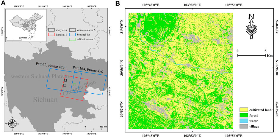
FIGURE 1. The study area and validation areas (A) Location of the study area and validation areas (B) Land cover map of the study area.

The validation area A is adjacent to the study area (Figure 1A), with similar terrain (average slope angle <13°) and surface vegetation coverage, and also does not belong to the “comfort zone” of Sentinel-1A InSAR deformation monitoring. The reliability of the established models were validated in this area.

The validation area B is located in the southeast of the study area (Figure 1A), with larger average slope angle and more lush vegetation cover, and the land surface type is mainly forest. The established models were validated in this area based on SAR data from different imaging perspectives to verify the reliability and universality of the models.

2.2 Data and data preprocessing

We collected an approximately cloud-free Landsat-8 Operational Land Imager (OLI) image (Table 1) taken in the summer to calculate the NDVI. The atmospheric correction and radiometric correction were first performed on the Landsat8 OLI image, and the image was cropped based on the vector boundaries of the study area and validation areas, then we calculated the NDVI (Figure 2) based on the following equation:

$\begin{array}{c}\mathit{N}\mathit{D}\mathit{V}\mathit{I}=\frac{{\mathit{P}}_{\mathit{N}\mathit{I}\mathit{R}}-{\mathit{P}}_{\mathit{R}\mathit{E}\mathit{D}}}{{\mathit{P}}_{\mathit{N}\mathit{I}\mathit{R}}+{\mathit{P}}_{\mathit{R}\mathit{E}\mathit{D}}}\end{array}(1)$

where $P_{NIR}$ and $P_{RED}$ represent the reflection of the near-infrared band and red band, corresponding to band-5 and band-4 of Landsat8 OLI, respectively. The NDVI varies between [−1, 1]: it is negative when the cloud cover is exceedingly high or the surface is covered with water or snow; zero when the surface is covered with rocks or bare soil; and positive when the surface is covered with vegetation, where increasing positive values are associated with increasing vegetation coverage.

TABLE 1

TABLE 1. Landsat-8 image.

FIGURE 2

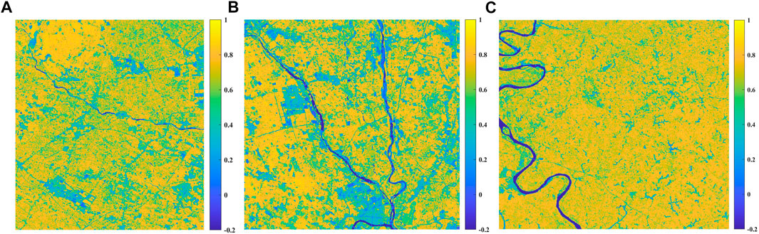
FIGURE 2. NDVI images (A) Study area (B) Validation area A (C) Validation area B.

For the SAR data, we collected descending Sentinel-1A images (Table 2) covering the study area and validation area A, and the data from different imaging perspective covering validation area B (Table 3), footprints of Sentinel-1A data we used are displayed in blue rectangle in Figure 1A. The following three preprocessing steps were performed. (1) Interferometric pair SLC interference was performed using double-pass differential interferometry, and precise orbit ephemerides and shuttle radar topography mission (SRTM) DEM (30 m) were used to correct the orbit errors and simulate the terrain phase, respectively. (2) Multi-look processing was performed to suppress speckle noise and ensure that the SAR images maintained the same resolution as the Landsat8 image. (3) The coherence was calculated and the contribution of the spatial decorrelation was removed according to the theoretical formula given in the literature (Lee and Liu, 2001). The theoretical model (Nasirzadehdizaji et al., 2021) of coherence is:

$\begin{array}{c}\mathit{\gamma }=\frac{\mathit{E}\left[{\mathit{\mu }}_{\mathbf{1}}{\mathit{\mu }}_{\mathbf{2}}^{*}\right]}{\sqrt{\mathit{E}\left[{\left|{\mathit{\mu }}_{\mathbf{1}}\right|}^{\mathbf{2}}\right]\mathit{E}\left[{\left|{\mathit{\mu }}_{\mathbf{2}}\right|}^{\mathbf{2}}\right]}}\end{array}(2)$

Where $\gamma$ indicates coherence, $E\left[\bullet \right]$ is the mathematical expectation and ${\mu }^{*}$ is the conjugate complex of the SLC image. However, thermal noise and other factors of the radar system can easily generate a jump in the calculation result. This causes the coherence to present a strong spatial fluctuation, which compromises the calculation

TABLE 2

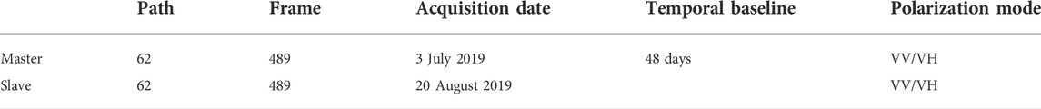
TABLE 2. Sentinel-1A images covering the study area and validation area A.

TABLE 3

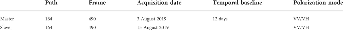
TABLE 3. Sentinel-1A images covering the validation area B.

accuracy. The coherence calculation scheme based on the amplitude data of the SAR. image can better resolve this problem. Although thermal noise decorrelation is generally ignored, this calculation strategy is still applied to minimize the ambiguity of the thermal noise on the coherence calculation results. The formulation is given as:

$\begin{array}{c}\mathit{\gamma }=\frac{{\displaystyle \sum }_{\mathit{n}=\mathbf{1}}^{\mathit{N}}{\displaystyle \sum }_{\mathit{m}=\mathbf{1}}^{\mathit{M}}\left|{\mathit{\mu }}_{\mathbf{1}}\left(\mathit{n},\mathit{m}\right)\right|\left|{\mathit{\mu }}_{\mathbf{2}}\left(\mathit{n},\mathit{m}\right)\right|}{\sqrt{{{\displaystyle \sum }_{\mathit{n}=\mathbf{1}}^{\mathit{N}}{\displaystyle \sum }_{\mathit{m}=\mathbf{1}}^{\mathit{M}}\left|{\mathit{\mu }}_{\mathbf{1}}\left(\mathit{n},\mathit{m}\right)\right|}^{\mathbf{2}}{{\displaystyle \sum }_{\mathit{n}=\mathbf{1}}^{\mathit{N}}{\displaystyle \sum }_{\mathit{m}=\mathbf{1}}^{\mathit{M}}\left|{\mathit{\mu }}_{\mathbf{2}}\left(\mathit{n},\mathit{m}\right)\right|}^{\mathbf{2}}}}\end{array}(3)$

where $M$ and $N$ are the sizes of the data blocks for calculating coherence, n and m are the row and column numbers in the data windows, ${\mu }_1\left(n,m\right)$ and ${\mu }_2\left(n,m\right)$ represent the complex values at the image coordinates (n, m) in the master and slave image data blocks, respectively, $\left|\bullet \right|$ is the absolute value of the complex, and ${\left|\cdot \right|}^2$ is the second-order norm of the data.

The coherence ranges from zero in the case of complete decorrelation (i.e., the interferometric phase is only noise) to one if the two signals are fully correlated (i.e., complete absence of phase noise). The coherence reaches the maximum value when the scatterer position and physical properties within the averaging window are the same for the two observations. In contrast, any differences in the scatterer position or properties in the interval between the two observations introduce a phase difference of two backscattered signals and accordingly cause the coherence value to decrease (Nasirzadehdizaji et al., 2021). After completing the coherence calculation, the coherence images were geocoded and co-registered with the NDVI image by SRTM DEM (30 m) and ground highly coherent points (HCPs), which displayed in Figure 3. The data preprocessing work flow is shown in Figure 4.

FIGURE 3

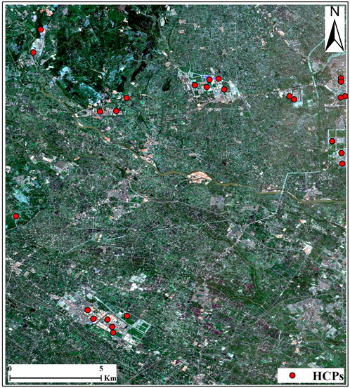
FIGURE 3. Distribution of ground highly coherent points (HCPs) in the study area. The background is 10-m resolution Sentinel-2 true-color image.

FIGURE 4

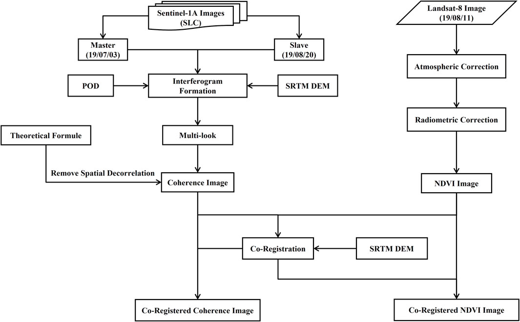
FIGURE 4. Data preprocessing work flow.

2.3 Contribution of temporal decorrelation to coherence

The coherence obtained in Section 2.2 removed the contribution of the spatial decorrelation, but the contribution of the temporal decorrelation should also be considered. Rocca et al. (Rocca, 2007) proposed an exponential decay function between the coherence and temporal baseline for C-band ERS-1 data, and assigned an exponential decay constant to the model to represent the decay rate of coherence with an increasing temporal baseline. A decay function of surface reflectors was thereafter proposed, which still maintains the correlation under a long-term temporal baseline (Parizzi et al., 2009). Other time-coherence decay functions have also been discussed (Krieger et al., 2007; Sica et al., 2019). The study area in this paper has dense vegetation and few highly coherent surface reflectors, thus the time-coherence decay function does not need to account for highly coherent ground objects. Multiple interferometric pairs were generated under the multi-master image strategy, the Sentinel-1A data used are displayed in Table 4. The results show that when the temporal baseline is less than 216 days, the VV-polarization coherence decays exponentially with increasing temporal baseline, whereas the VV-polarization coherence shows no notable decay trend when the temporal baseline exceeds 216 days and fluctuates around a stable value (Figure 5A). Figure 5B shows that the VH-polarization coherence also decays exponentially with increasing temporal baseline when it is less than 168 days. If the temporal baseline exceeds 168 days, the VH-polarization coherence fluctuates around another stable value, and also exhibits no clear decay trend. We therefore define 216 and 168 days as the critical exponent decay temporal baselines for this study. The coefficients $A1$, $t1$, $A2$, and $t2$ shown in Figure 5 were obtained as 0.743, 206 days, 0.560, and 222 days, respectively. The two stable values around which the coherence fluctuated are 0.370 and 0.325, respectively.

TABLE 4

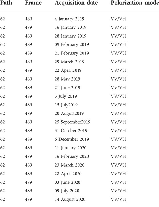
TABLE 4. Sentinel-1A images used in the multi-master image strategy.

FIGURE 5

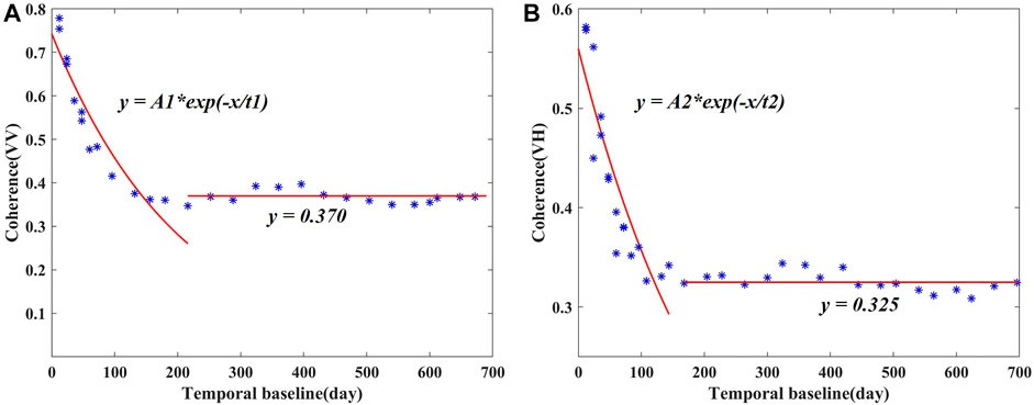
FIGURE 5. Relationship between the temporal baseline and coherence (A) VV channel (B) VH channel.

2.4 Model building based on the absolute value of the Pearson correlation coefficient

All of the pixels in the NDVI image and coherence images were initially involved in the analysis; however, we found that large global errors were introduced and reliable relationships could not be established. We therefore applied the window sampling method proposed in the literature (Chen et al., 2021) to account for the coherence value is related with the window size (Zhang et al., 2018). The steps of this method are as follows. (1) Set a moving window to sample the NDVI image, and a second moving window of the same size to simultaneously sample the coherence image until the two windows traverse the two images, respectively. (2) Calculate the Pearson correlation coefficient (Pearson, 1895) between the NDVI pixels and coherence pixels in the two windows based on Eq. 4.

$\begin{array}{c}\mathit{\rho }\left(\mathit{X},\mathit{Y}\right)=\frac{{\displaystyle \sum }_{\mathit{i}=\mathbf{1}}^{\mathit{n}}\left({\mathit{X}}_{\mathit{i}}-\overline{\mathit{X}}\right)\left({\mathit{Y}}_{\mathit{i}}-\overline{\mathit{Y}}\right)}{\sqrt{{\displaystyle \sum }_{\mathit{i}=\mathbf{1}}^{\mathit{n}}{\left({\mathit{X}}_{\mathit{i}}-\overline{\mathit{X}}\right)}^{\mathbf{2}}}\sqrt{{\displaystyle \sum }_{\mathit{i}=\mathbf{1}}^{\mathit{n}}{\left({\mathit{Y}}_{\mathit{i}}-\overline{\mathit{Y}}\right)}^{\mathbf{2}}}}\end{array}(4)$

where $\rho \left(X,Y\right)$ represents the Pearson correlation coefficient, $X_i$ represents the elements in a dataset, $\overline{X}$ is the mean value of the elements in this dataset, and $Y_i$ and $\overline{Y}$ are the elements and mean value of another dataset, respectively. (3) Set a threshold: if the Pearson correlation coefficient between the two windows meet the preset threshold, the pixels in the two windows are retained for subsequent analysis; otherwise, all pixels in the two windows are abandoned. The above method was used to build a quantitative model between the NDVI and L-band ALOS-1/PALSAR-1 coherence. For the C-band Sentinel-1A data, the strong negative linear correlation between the NDVI and coherence was revealed in preliminary experiments, showing a linear decrease of the coherence with increasing surface vegetation coverage. This method thus directly ignores numerous pixels with a negative linear correlation and significantly reduces the accuracy of the established models.

We therefore improved the correlation measurement of the two windows using the above method by calculating the absolute value of the Pearson correlation coefficient (marked as T) of the pixels in the two windows to account for the large number of pixels with a negative linear correlation. When the T value of the pixels in the two windows is greater than or equal to the preset threshold (marked as T0), these pixels are retained and participate in the subsequent analysis; otherwise, they are abandoned and not included in the analysis. Numerous experiments revealed that this window sampling method with the improved correlation measurement can significantly increase the accuracy of the quantitative relationship between the Landsat8-derived NDVI and Sentinel-1A coherence. The ideal sampling window size and threshold for VV- and VH-polarization were also obtained. The window sampling method with the improved correlation measurement is shown in Figure 6, the top and bottom pictures represent the NDVI and coherence image, respectively. T is the absolute value of the Pearson correlation coefficient, and T0 is the preset threshold.

FIGURE 6

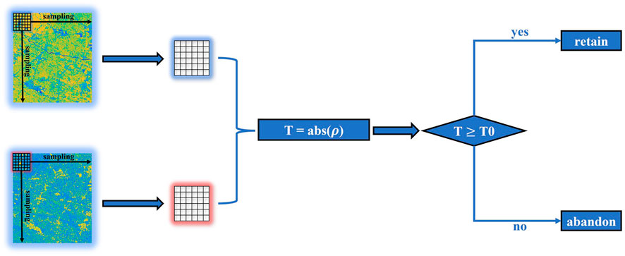
FIGURE 6. Window sampling method with improved correlation measurement.

We have found that the size of the sampling window is positively proportional to the amount of data that meet the threshold. when the sampling window size is small (less than 5$\times$5), there is a significant linear relationship between the two variables, however, the global error of the models obtained after fitting are significant. The amount of data that meet the threshold are numerous in terms of the sampling window size are large (more than 10$\times$10), and there is no obvious functional relationship between the two variables. Tables 5, 6 respectively display the determination coefficient (R2) and root mean square error (RMSE) of the optimal fitting function corresponding to each threshold when the sampling window is between 5$\times$5 and 9$\times$9 at VV and VH channels, then we obtain the optimal sampling window size and threshold at two polarization channels considering the accuracy of the fitting function and the global error of the models after fitting. The optimal sampling window size is 5$\times$5 for VV-polarization and the threshold is 0.7, whereas the optimal values for VH-polarization are 9$\times$9 and 0.6, respectively. All of the pixels that met the preset threshold were retained, and then some abnormal pixels are artificially abandoned.

TABLE 5

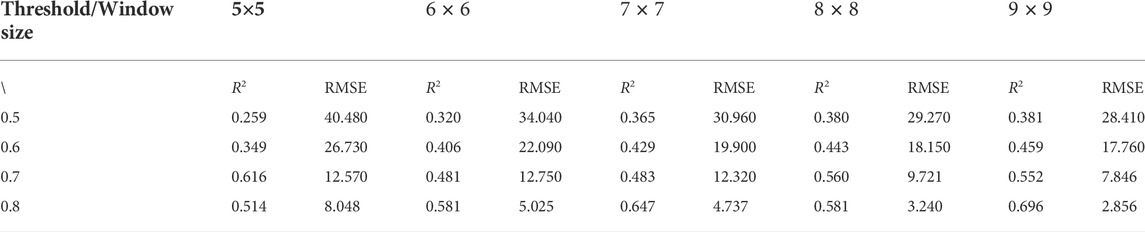
TABLE 5. performance of different sampling window size and threshold at VV channel.

TABLE 6

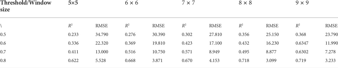
TABLE 6. performance of different sampling window size and threshold at VH channel.

Then we get the relationships between the Landsat8-derived NDVI and Sentinel-1A coherence of the retained pixels, as shown in Figure 7.

FIGURE 7

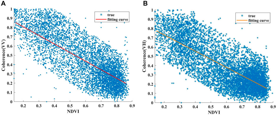
FIGURE 7. Relationship between the Landsat8-derived NDVI and Sentinel-1A coherence (A) VV channel (B) VH channel.

Section 2.3 discussed the relationship between the coherence and temporal baseline. The results indicate an exponential decay effect of the temporal decorrelation on the coherence, and that the critical temporal baseline of the VV- and VH-polarization coherences are 216 and 168 days, respectively. The temporal baseline of the interferometric pair used in this study is 48 days (Table 2). In this study, inspired by the work of Chen et al. (Chen et al., 2021), it is necessary to add a temporal decay factor to the models to improve their reliability. We then obtained a second-order linear model between the Landsat8-derived NDVI and Sentinel-1A coherence (VV) as follows:

$\begin{array}{c}\mathit{\gamma }\mathbf{1}=\{\begin{array}{c}\mathbf{0},-\mathbf{1}<\mathit{N}\mathit{D}\mathit{V}\mathit{I}<\mathbf{0.15},\mathit{N}\mathit{D}\mathit{V}\mathit{I}>\mathbf{0.87}\\ \mathit{a}\mathbf{1}\bullet \mathit{exp}\left(-\frac{\mathit{x}}{\mathit{t}\mathbf{1}}\right)\bullet \mathit{N}\mathit{D}\mathit{V}\mathit{I}+\mathit{b}\mathbf{1},\mathbf{0.15}\le \mathit{N}\mathit{D}\mathit{V}\mathit{I}\le \mathbf{0.87}\end{array}\end{array}(5)$

where $\gamma 1$ and $x$ represent the coherence (VV) and temporal baseline of the interferometric pair, respectively, $\mathit{exp}\left(-x/t1\right)$ and $t1$ represent the temporal decay factor and exponential decay speed factor of the coherence (VV), respectively, and $a1$ and $b1$ are parameters to be estimated. In this study, $x$ = 48 days (Table 2) and $t1$ = 206 days (Section 2.3).

A significant negative linear relationship was also observed between the Landsat8-derived NDVI and Sentinel-1A coherence (VH). The coherence (VH) was found to linearly decrease with increasing NDVI at a slightly lower rate than that of the coherence (VV). The second-order linear model between the Landsat8-derived NDVI and Sentinel-1A coherence (VH) is given as:

$\begin{array}{c}\mathit{\gamma }\mathbf{2}=\{\begin{array}{c}\mathbf{0},-\mathbf{1}<\mathit{N}\mathit{D}\mathit{V}\mathit{I}<\mathbf{0.14},\mathit{N}\mathit{D}\mathit{V}\mathit{I}>\mathbf{0.89}\\ \mathit{a}\mathbf{2}\bullet \mathbf{exp}\left(-\frac{\mathit{x}}{\mathit{t}\mathbf{2}}\right)\bullet \mathit{N}\mathit{D}\mathit{V}\mathit{I}+\mathit{b}\mathbf{2},\mathbf{0.14}\le \mathit{N}\mathit{D}\mathit{V}\mathit{I}\le \mathbf{0.89}\end{array}\end{array}(6)$

where $\gamma 2$ and $x$ represent the coherence (VH) and temporal baseline of the interferometric pair, respectively, $\mathit{exp}\left(-x/t2\right)$ and $t1$ represent the temporal decay factor and exponential decay speed factor of the coherence (VH), respectively, and $a2$ and $b2$ are parameters to be estimated.

The least squares method is used to fit the two formulas to improve the robustness, thus yielding two quantitative models between the Landsat8-derived NDVI and Sentinel-1A coherence. The obtained parameters are $a1$ = −1.168, $b1$ = 0.992, $a2$ = −1.086, and $b2$ = 0.905.

3 Results and discussion

3.1 Results and error analysis

Eq. 3 was used to calculate the true VV-polarization coherence image (Figure 8A) of the study area according to the amplitude information, and Eq. 5 was applied to estimate the VV-polarization coherence image (Figure 8B) using the Landsat8-derived NDVI. For VH-polarization coherence, Eq. 3 was used to calculate the true coherence image (Figure 8C) and estimate the coherence (Figure 8D) based on the model given in Eq. 6 of the study area. The differences distribution obtained by subtracting the estimated coherence from the true coherence in VV-polarization and VH-polarization are displayed in Figures 8E, F, respectively. It can be found that the differences distribution in VV-polarization are uniformly distributed without significant concentrated error, whereas those in VH-polarization are mainly concentrated in the red circle (village distribution area) of Figure 8F.

FIGURE 8

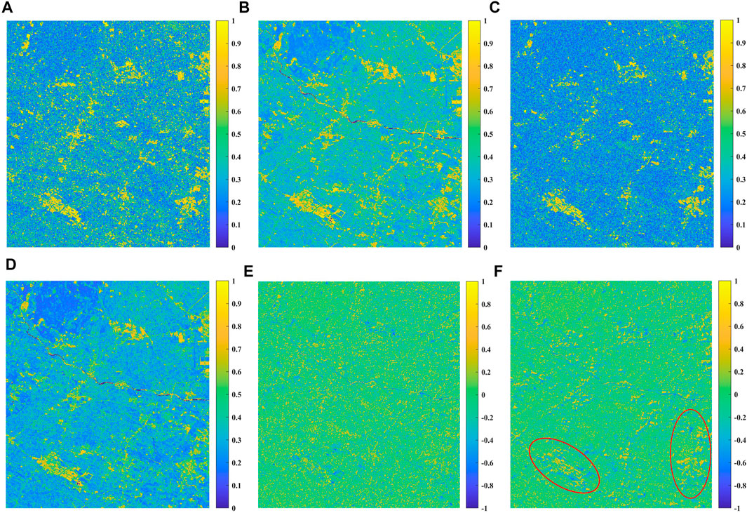
FIGURE 8. Coherence images of the study area (A) True at VV channel (B) Estimation at VV channel (C) True at VH channel (D) Estimation at VH channel (E) Differences distribution at VV channel (F) Differences distribution at VH channel.

As shown in Figure 9A, the mean error in VV-polarization is -0.037 with a standard deviation of 0.205. Most of the errors distribute between −0.3 and 0.3, and the global errors obey a normal distribution. Figure 9B shows that the mean error in VH-polarization is −0.045 with a standard deviation of 0.201, and the global errors still obey the normal distribution.

FIGURE 9

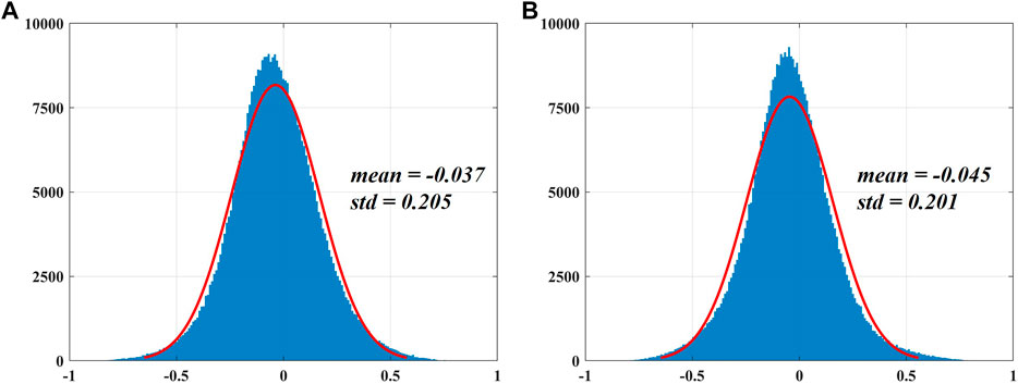
FIGURE 9. The error histogram of the study area (A) VV channel (B) VH channel.

3.2 Models validation

3.2.1 Performance of established models in validation area A

We performed the same experiments in the validation area A to consider the model reliability using consistent data and data processing methods as those in the study area We then obtained the true VV-polarization coherence image (Figure 10A) and estimated the VV-polarization coherence image (Figure 10B) of the validation area. Those in VH- polarization are displayed in Figures 10C, D, respectively. Figures 10E, F give the differences distribution in validation area were obtained by subtracting the estimated coherence from the true coherence. It can be found that relatively large errors are concentrated in villages and river distribution areas, as shown in the red circle in Figures 10E, F. Figure 11A shows that the mean error in VV-polarization is -0.067 with a standard deviation of 0.256, most of the errors distribute between −0.4 and 0.4 and basically obey a normal distribution. As shown in Figure 11B, the mean error in VH-polarization is −0.065 with a standard deviation of 0.230, these errors are larger and more discrete than those in the study area on the whole, but still roughly obey a normal distribution and mostly distribute between −0.35 and 0.35. Based on the error distribution in the study area and validation area A, it is confirmed that the models given in Eq. 5–6 are reliable without significant trend and random error.

FIGURE 10

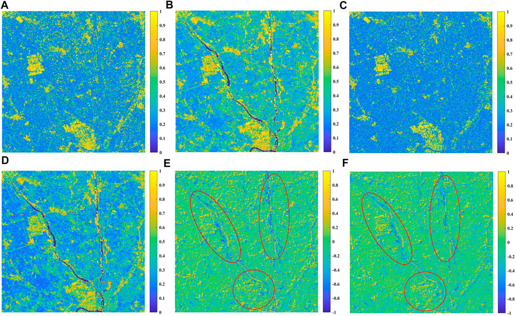
FIGURE 10. Coherence images of the validation A (A) True at VV channel (B) Estimation at VV channel (C) True at VH channel (D) Estimation at VH channel (E) Differences distribution at VV channel (F) Differences distribution at VH channel.

FIGURE 11

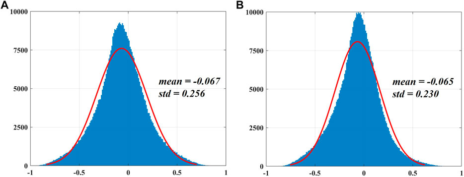
FIGURE 11. The error histogram of the validation area A (A) VV channel (B) VH channel.

3.2.2 Performance of established models in validation area B

We used Sentinel-1A images from different imaging perspectives covering validation area B that were independent from the study area and validation area A regard of the reliability and universality of the models, the data processing method is consistent with the study area and validation area A. As observed in Figure 12, the true coherence images at the two polarization channels are similar to the estimated coherence images, and the errors are mainly distributed in the river region, even though these areas are generally not included in the scope of InSAR ground deformation monitoring. Consistent with the study area and validation area A, we counted the error distribution of the validation area B. For errors statistics, Figure 13A shows that the errors of the validation area B at the VV channel are concentrated between -0.4 and 0.4 with the mean value and standard deviation are 0.040 and 0.190, respectively. The error distribution basically follows a normal distribution and no obvious random error existing. Those in VH-polarization are displayed in Figure 13B, most of the errors at VH channel distribute between -0.35 and 0.35 with the mean value and standard deviation are −0.020 and 0.193, respectively, and the global error still basically obeys the normal distribution. Based on the above distribution of differences and errors statistics, it allows us to confirm that the established models perform well in validation area B, and indicates the universality and dataset independence of the models to a certain extent.

FIGURE 12

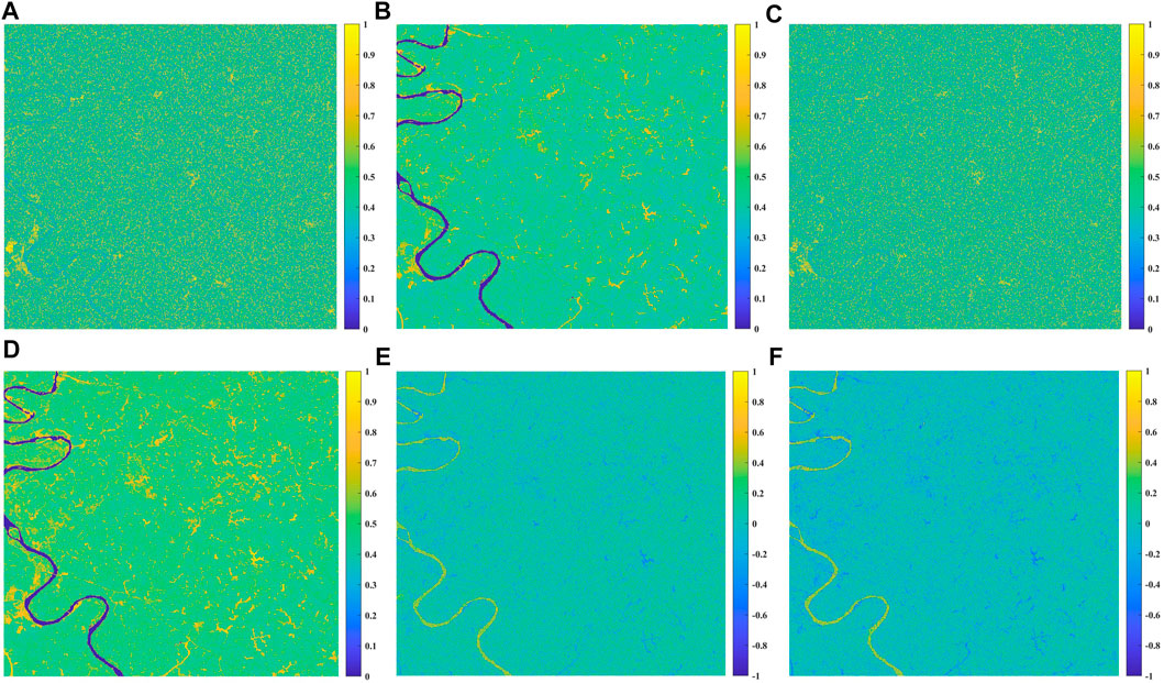
FIGURE 12. Coherence images of the validation area B (A) True at VV channel (B) Estimation at VV channel (C) True at VH channel (D) Estimation at VH channel (E) Differences distribution at VV channel (F) Differences distribution at VH channel.

FIGURE 13

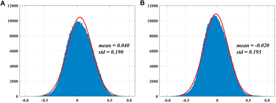
FIGURE 13. The error histogram of the validation area B (A) VV channel (B) VH channel.

3.3 Discussion

Figures 8A,C indicate that the VV-polarization coherence of the study area is higher than that of the VH-polarization on the whole owing to its high sensitivity to volume scattering, which strongly depends on the geometrical alignment and vegetation characteristics (Gao et al., 2017). The surface coverage of the study area is also mainly cultivated lands, followed by woodlands. The main crop of the cultivated lands is rice, for which the biophysical parameters have been shown to have a stronger relationship with VH-polarization than with VV-polarization (Wali et al., 2020). The VH-polarization radar signal is therefore more sensitive to rice than the VV-polarization radar signal. The decorrelation of the VH-polarization radar signal is accordingly more severe and the overall coherence is lower for the same temporal baseline.

The accuracy of the models in the study area is found to be higher than that in the validation area A, owing to the smaller and more concentrated global errors, for both VV-polarization and VH-polarization. However, the same interferometric pairs are used in the study area and validation area A, thus the differences of the spatial decorrelation and temporal decorrelation caused by different imaging geometry and temporal baselines of the interferometric pair are excluded. We interpret there to be two reasons for the higher model accuracy in the study area. (1) Although the topography of the study area is similar to the validation area A, slight differences still remain. The terrain fluctuation and average slope (average slope angle <13°) in the validation area are slightly gentler than those in the study area, thus the spatial decorrelation errors caused by slight terrain differences may reduce the model accuracy in the validation area, even if the contribution of the spatial decorrelation is removed from the models. (2) The estimated coherence of water system areas are zero based on the established models. There are two rivers in the validation area A where the true coherence is almost zero. Thus, owing to the limited number of samples within the coherence estimation window, the underestimation bias in the low coherence area leads to a random distribution of pixels within the completely decorrelated areas. Apart from this, although the optimal sampling window size and threshold for the two polarization modes were obtained experimentally, the number of pixels participating in the VH-polarization model fitting analysis was still more than that in the VV-polarization model and the distribution was more discrete, resulting in a lower model accuracy. The VV-polarization model accuracy is therefore better than that of the VH channel in both the study area and the validation area A.

The performance of the established models in the validation area B shows their universality and dataset independence under different imaging geometry. Like the validation area A, the estimated coherence errors at the two polarization channels are still mainly concentrated in the river distribution area, and there is no obvious error trend and random error in other areas within the validation area B, however, in a broader context, the established models need to be verified in wider areas and richer dataset under different imaging geometry to further illustrate their robustness and universality.

The established models still have some weaknesses in terms of the different abovementioned perspectives. We suggest that the following improvements be made in subsequent study. (1) Although the contribution of spatial decorrelation was removed in the models, slight topographic differences between the different areas can still introduce spatial decorrelation errors into the models. A method to completely remove the contribution of spatial decorrelation must therefore be considered to improve the model universality. (2) We defined the exponent decay critical temporal baseline as 216 and 168 days for Sentinel-1A VV- and VH-polarization coherence, respectively. These two critical values are greater than 48 and 12 days of the temporal baseline for the interferometric pairs used in this study. It is thus reasonable to add a temporal decay factor to the models. On the contrary, if the temporal baseline exceeds the exponential decay critical temporal baseline, (i.e., when the coherence decays to a low level with no notable decay trend), it is unreasonable to add such a decay factor. It is therefore important to establish a more reliable relationship between the coherence and interferometric pair temporal baseline in the case of a long-term application to improve the model accuracy, even if such a long-term baseline is not suitable for traditional InSAR surface deformation monitoring in vegetated area of C-band sentinel-1A data. (3) Rivers inevitably exist in some vegetated areas, thus a quantitative relationship between the water indexes and coherence must be established and incorporated into the models to improve their robustness. Other factors should also be considered to improve the models. For example, the weather conditions in the study area leads to refractivity of the atmosphere through which a traveling radar wave imparts a phase delay (or advance) that can vary in both space and time owing to the dependence of refractivity on various atmospheric properties (Wadge et al., 2010). These induced propagation delays (or advances) affect the quality of the interference fringe and coherence calculation. Furthermore, different response characteristics of the different vegetation types to the SAR echo signals will also lead to differing coherence and decorrelation (Zhang et al., 2016), which will be constructed in future models.

4 Conclusion

This study establishes two second-order linear models between the Landsat8-derived NDVI and Sentinel-1A coherence in co- and cross-polarization that reveal the relationship between InSAR decorrelation and vegetation coverage. Coherence is found to linearly decrease with increasing vegetation coverage, and the linear trend differs depending on the co-polarization and cross-polarization mode. The two models were validated simultaneously using similar data in the validation area A and independent imaging geometry data in the validation area B. The NDVI obtained from free optical satellites can therefore be used to estimate the coherence prior to performing InSAR processing on vegetated areas to monitor the surface deformation (i.e., prior to the interferometric pair’s SLC interference) to quantitatively estimate the decorrelation of these areas. The SAR data selection can be determined using quantitative models prior to interference, thereby increasing the research productivity and reducing the time and economic costs. This study fills the gap of the above models in C-band SAR data, in addition to the C-band Sentinel-1A data, the quantitative relationship between the NDVI and L-band co-polarization ALOS-1/PALSAR-1 coherence has been established (29), and other quantitative models should be constructed for the L-band and X-band SAR data at different polarization channels in the future.

Data availability statement

The raw data supporting the conclusions of this article will be made available by the authors, without undue reservation.

Author contributions

RZ: Conceptualization; Methodology; Formal analysis; Data curation; Writing–original draft, review, and editing. JP: Formal analysis; Funding acquisition; Supervision. ZX: Funding acquisition. ZC: Conceptualization; Methodology. YY: Writing–original draft, review, and editing.

Funding

This work was supported by Key R&D Program of Ningxia Autonomous Region: Ecological environment monitoring and platform development of ecological barrier protection system for Helan Mountain (ID: 2022CMG02014) and Scientific research project managed by Guizhou bureau of Geology and mineral resources in 2019: key technology and application of ecological environment monitoring of mountains, rivers, forests, fields, lakes and grasses - Taking Bailidujuan as an example (ID: 201909).

Acknowledgments

Thanks to Yaogang Chen of Central South University for his helpful and efficient guidance. The Sentinel-1A data and Landsat-8 data were provided by ESA and USGS, respectively.

Conflict of interest

Author ZX was employed by the company China Railway Eryuan Engineering Group CO.LTD.

The remaining authors declare that the research was conducted in the absence of any commercial or financial relationships that could be construed as a potential conflict of interest.

Publisher’s note

All claims expressed in this article are solely those of the authors and do not necessarily represent those of their affiliated organizations, or those of the publisher, the editors and the reviewers. Any product that may be evaluated in this article, or claim that may be made by its manufacturer, is not guaranteed or endorsed by the publisher.

Reference

Abdel-Hamid, A., Dubovyk, O., and Greve, K. (2021). The potential of sentinel-1 InSAR coherence for grasslands monitoring in Eastern Cape, South Africa. International Journal of Applied Earth Observation and Geoinformation 98, 102306. doi:10.1016/j.jag.2021.102306

CrossRef Full Text | Google Scholar

Amani, M., Poncos, V., Brisco, B., Foroughnia, F., DeLancey, E. R., and Ranjbar, S. (2021). InSAR Coherence Analysis for Wetlands in Alberta, Canada Using Time-Series Sentinel-1 Data. Remote Sensing 13, 3315. doi:10.3390/rs13163315

CrossRef Full Text | Google Scholar

Anh, N., and Hang, N. (2019). Deforestation Detection Using Sentinel-1 Time-Series Case Study In Quang Son -Dak Glong District. Dak Nong Province. doi:10.13140/RG.2.2.28003.09761

CrossRef Full Text | Google Scholar

Arab-Sedze, M., Heggy, E., Bretar, F., Berveiller, D., and Jacquemoud, S. (2014). Quantification of L-band InSAR coherence over volcanic areas using LiDAR and in situ measurements. Remote Sensing of Environment 152, 202–216. doi:10.1016/j.rse.2014.06.011

CrossRef Full Text | Google Scholar

Bai, Z., Fang, S., Gao, J., Zhang, Y., Jin, G., Wang, S., et al. (2020). Could Vegetation Index be Derive from Synthetic Aperture Radar? – The Linear Relationship between Interferometric Coherence and NDVI. Sci. Rep. 10, 6749. doi:10.1038/s41598-020-63560-0

PubMed Abstract | CrossRef Full Text | Google Scholar

Bato, M. G., Lundgren, P., Pinel, V., Solidum, R., Daag, A., and Cahulogan, M. (2021). The 2020 Eruption and Large Lateral Dike Emplacement at Taal Volcano, Philippines: Insights From Satellite Radar Data. Geophys. Res. Lett. 48. doi:10.1029/2021GL092803

CrossRef Full Text | Google Scholar

Blaes, X., and Defourny, P. (2003). Retrieving crop parameters based on tandem ERS 1/2 interferometric coherence images. Remote Sensing of Environment 88, 374–385. doi:10.1016/j.rse.2003.08.008

CrossRef Full Text | Google Scholar

Canisius, F., Brisco, B., Murnaghan, K., Van Der Kooij, M., and Keizer, E. (2019). SAR Backscatter and InSAR Coherence for Monitoring Wetland Extent, Flood Pulse and Vegetation: A Study of the Amazon Lowland. Remote Sensing 11, 720. doi:10.3390/rs11060720

CrossRef Full Text | Google Scholar

Chen, Y., Sun, Q., and Hu, J. (2021). Quantitatively Estimating of InSAR Decorrelation Based on Landsat-Derived NDVI. Remote Sensing 13, 2440. doi:10.3390/rs13132440

CrossRef Full Text | Google Scholar

Corsa, B., Barba-Sevilla, M., Tiampo, K., and Meertens, C. (2022). Integration of DInSAR Time Series and GNSS Data for Continuous Volcanic Deformation Monitoring and Eruption Early Warning Applications. Remote Sensing 14, 784. doi:10.3390/rs14030784

CrossRef Full Text | Google Scholar

Xu, X., Sandwell, D. T., and Smith‐Konter, B. (2020). Coseismic Displacements and Surface Fractures from Sentinel‐1 InSAR: 2019 Ridgecrest Earthquakes. Seismological Research Letters 91, 1979–1985. doi:10.1785/0220190275

CrossRef Full Text | Google Scholar

Dai, K., Li, Z., Tomás, R., Liu, G., Yu, B., Wang, X., et al. (2016). Monitoring activity at the Daguangbao mega-landslide (China) using Sentinel-1 TOPS time series interferometry. Remote Sensing of Environment 186, 501–513. doi:10.1016/j.rse.2016.09.009

CrossRef Full Text | Google Scholar

Diniz, J. M. F. de S., Gama, F. F., and Adami, M. (2022). Evaluation of polarimetry and interferometry of sentinel-1A SAR data for land use and land cover of the Brazilian Amazon Region. Geocarto International 37, 1482–1500. doi:10.1080/10106049.2020.1773544

CrossRef Full Text | Google Scholar

Engdahl, M. E., Borgeaud, M., and Rast, M. (2001). The use of ERS-1/2 Tandem interferometric coherence in the estimation of agricultural crop heights. IEEE Trans. Geosci. Remote Sens. 39, 1799–1806. doi:10.1109/36.942558

CrossRef Full Text | Google Scholar

Flynn, T., Tabb, M., and Carande, R. (2002). Coherence region shape extraction for vegetation parameter estimation in polarimetric SAR interferometry. IEEE International Geoscience and Remote Sensing Symposium 5, 2596–2598.

Google Scholar

Gao, Q., Zribi, M., Escorihuela, M. J., and Baghdadi, N. (2017). Synergetic Use of Sentinel-1 and Sentinel-2 Data for Soil Moisture Mapping at 100 m Resolution. Sensors 17, 1966. doi:10.3390/s17091966

PubMed Abstract | CrossRef Full Text | Google Scholar

Guo, Q., Xu, C., Wen, Y., Liu, Y., and Xu, G. (2019). The 2017 Noneruptive Unrest at the Caldera of Cerro Azul Volcano (Galápagos Islands) Revealed by InSAR Observations and Geodetic Modelling. Remote Sensing 11, 1992. doi:10.3390/rs11171992

CrossRef Full Text | Google Scholar

Guo, Z., Qi, W., Huang, Y., Zhao, J., Yang, H., Koo, V.-C., et al. (2022). Identification of Crop Type Based on C-AENN Using Time Series Sentinel-1A SAR Data. Remote Sensing 14, 1379.

CrossRef Full Text | Google Scholar

Hall-Atkinson, C., Smith, L. C., and Mackenzie, (2001). Delineation of delta ecozones using interferometric SAR phase coherence, 78, 229–238. doi:10.1016/S0034-4257(01)00221-8River Delta, N.W.T., CanadaRemote Sensing of Environment

CrossRef Full Text | Google Scholar

Han, B., Yang, C., Li, Z., Yu, C., Zhao, C., and Zhang, Q. (2022). Coseismic and postseismic deformation of the 2016 Mw 6.0 Petermann ranges earthquake from satellite radar observations. Advances in Space Research 69, 376–385.

CrossRef Full Text | Google Scholar

He, Y., Wang, W., Yan, H., Zhang, L., Chen, Y., and Yang, S. (2020). Characteristics of Surface Deformation in Lanzhou with Sentinel-1A TOPS. Geosciences 10, 99. doi:10.3390/geosciences10030099

CrossRef Full Text | Google Scholar

Jiang, M., Ding, X., Li, Z., Tian, X., Wang, C., and Zhu, W. (2014). InSAR Coherence Estimation for Small Data Sets and Its Impact on Temporal Decorrelation Extraction. IEEE Trans. Geosci. Remote Sens. 52, 6584–6596. doi:10.1109/TGRS.2014.2298408

CrossRef Full Text | Google Scholar

Jung, J., Kim, D., Lavalle, M., and Yun, S.-H. (2016). Coherent Change Detection Using InSAR Temporal Decorrelation Model: A Case Study for Volcanic Ash Detection. IEEE Trans. Geosci. Remote Sens. 54, 5765–5775. doi:10.1109/TGRS.2016.2572166

CrossRef Full Text | Google Scholar

Krieger, G., Moreira, A., Fiedler, H., Hajnsek, I., Werner, M., Younis, M., et al. (2007). TanDEM-X: A Satellite Formation for High-Resolution SAR Interferometry. IEEE Trans. Geosci. Remote Sens. 45, 3317–3341.

CrossRef Full Text | Google Scholar

Kumar, V., Huber, M., Rommen, B., and Steele-Dunne, S. C. (2022). Agricultural SandboxNL: A national-scale database of parcel-level processed Sentinel-1 SAR data. Sci. Data 9, 402. doi:10.1038/s41597-022-01474-4

PubMed Abstract | CrossRef Full Text | Google Scholar

Lee, H., and Liu, J. G. (2001). Analysis of topographic decorrelation in SAR interferometry using ratio coherence imagery. IEEE Trans. Geosci. Remote Sens. 39, 223–232. doi:10.1109/36.905230

CrossRef Full Text | Google Scholar

Liang, D., Guo, H., Zhang, L., Cheng, Y., Zhu, Q., and Liu, X. (2021a). Time-series snowmelt detection over the Antarctic using Sentinel-1 SAR images on Google Earth Engine. Remote Sensing of Environment 256, 112318. doi:10.1016/j.rse.2021.112318

CrossRef Full Text | Google Scholar

Liang, H., Zhang, L., Ding, X., Lu, Z., Li, X., Hu, J., et al. (2021b). Suppression of Coherence Matrix Bias for Phase Linking and Ambiguity Detection in MTInSAR. IEEE Trans. Geosci. Remote Sensing 59, 1263–1274. doi:10.1109/TGRS.2020.3000991

CrossRef Full Text | Google Scholar

Manjula, T. R., Ramesh, A., Unnikrishnan, L., Reddy, V. C., Sethia, G., Nagarjan, N., et al. (2022). “Temporal Variation of Glacier Melting Rate of Helheim and Gangotri Glaciers Using Sentinel 1A Images,” in Advanced Computational Paradigms and Hybrid Intelligent Computing Advances in Intelligent Systems and Computing. Editors T. K. Gandhi, D. Konar, B. Sen, and K. Sharma (Singapore: Springer), 231–239. doi:10.1007/978-981-16-4369-9_24

CrossRef Full Text | Google Scholar

Merchant, M. A., Obadia, M., Brisco, B., DeVries, B., and Berg, A. (2022). Applying Machine Learning and Time-Series Analysis on Sentinel-1A SAR/InSAR for Characterizing Arctic Tundra Hydro-Ecological Conditions. Remote Sensing 14, 1123. doi:10.3390/rs14051123

CrossRef Full Text | Google Scholar

Nasirzadehdizaji, R., Cakir, Z., Balik Sanli, F., Abdikan, S., Pepe, A., and Calò, F. (2021). Sentinel-1 interferometric coherence and backscattering analysis for crop monitoring. Computers and Electronics in Agriculture 185, 106118. doi:10.1016/j.compag.2021.106118

CrossRef Full Text | Google Scholar

Nikaein, T., Iannini, L., Molijn, R. A., and Lopez-Dekker, P. (2021). On the Value of Sentinel-1 InSAR Coherence Time-Series for Vegetation Classification. Remote Sensing 13, 3300. doi:10.3390/rs13163300

CrossRef Full Text | Google Scholar

Parizzi, A., Cong, X., and Eineder, M. (2009). First Results from Multifrequency Interferometry. A comparison of different decorrelation time constants at L, C, and X Band. ESA Scientific Publications Frascati, 1. –5.

Google Scholar

Pearson, K. (1895). Correlation coefficient. Royal Society Proceedings, 214.

Google Scholar

Pinto, N., Simard, M., and Dubayah, R. (2013). Using InSAR Coherence to Map Stand Age in a Boreal Forest. Remote Sensing 5, 42–56. doi:10.3390/rs5010042

CrossRef Full Text | Google Scholar

Potin, P., Rosich, B., Grimont, P., Miranda, N., Shurmer, I., O’Connell, A., et al. (2016). Sentinel-1 Mission Status. Proceedings of EUSAR 2016: 11th European Conference on Synthetic Aperture Radar. 1–6.

Google Scholar

Rocca, F. (2007). Modeling Interferogram Stacks. IEEE Trans. Geosci. Remote Sens. 45, 3289–3299. doi:10.1109/TGRS.2007.902286

CrossRef Full Text | Google Scholar

Santoro, M., Wegmuller, U., and Askne, J. I. H. (2010). Signatures of ERS–Envisat Interferometric SAR Coherence and Phase of Short Vegetation: An Analysis in the Case of Maize Fields. IEEE Trans. Geosci. Remote Sens. 48, 1702–1713. doi:10.1109/TGRS.2009.2034257

CrossRef Full Text | Google Scholar

Sedze, M., Heggy, E., Bretar, F., Berveiller, D., and Jacquemoud, S. (2012). L-band InSAR decorrelation analysis in volcanic terrains using airborne LiDAR data and in situ measurements: The case of the Piton de la Fournaise volcano, France. IEEE International Geoscience and Remote Sensing Symposium, 3907–3910. doi:10.1109/IGARSS.2012.6350558

CrossRef Full Text | Google Scholar

Sica, F., Pulella, A., Nannini, M., Pinheiro, M., and Rizzoli, P. (2019). Repeat-pass SAR interferometry for land cover classification: A methodology using Sentinel-1 Short-Time-Series. Remote Sensing of Environment 232, 111277. doi:10.1016/j.rse.2019.111277

CrossRef Full Text | Google Scholar

Suresh, D., and Yarrakula, K. (2020). InSAR based deformation mapping of earthquake using Sentinel 1A imagery. Geocarto International 35, 559–568. doi:10.1080/10106049.2018.1544289

CrossRef Full Text | Google Scholar

Tampuu, T., Praks, J., Kull, A., Uiboupin, R., Tamm, T., and Voormansik, K. (2021). Detecting peat extraction related activity with multi-temporal Sentinel-1 InSAR coherence time series. International Journal of Applied Earth Observation and Geoinformation 98, 102309. doi:10.1016/j.jag.2021.102309

CrossRef Full Text | Google Scholar

Wadge, G., Zhu, M., Holley, R. J., James, I. N., Clark, P. A., Wang, C., et al. (2010). Correction of atmospheric delay effects in radar interferometry using a nested mesoscale atmospheric model. Journal of Applied Geophysics 72, 141–149. doi:10.1016/j.jappgeo.2010.08.005

CrossRef Full Text | Google Scholar

Wali, E., Tasumi, M., and Moriyama, M. (2020). Combination of Linear Regression Lines to Understand the Response of Sentinel-1 Dual Polarization SAR Data with Crop Phenology—Case Study in Miyazaki, Japan. Remote Sensing 12, 189. doi:10.3390/rs12010189

CrossRef Full Text | Google Scholar

Wang, R., Dong, P., Dong, G., Xiao, X., Huang, J., Yang, L., et al. (2022). Exploring the impacts of street-level greenspace on stroke and cardiovascular diseases in Chinese adults. Ecotoxicology and Environmental Safety 243, 113974. doi:10.1016/j.ecoenv.2022.113974

PubMed Abstract | CrossRef Full Text | Google Scholar

Wang, T., Liao, M., and Perissin, D. (2010). InSAR Coherence-Decomposition Analysis. IEEE Geosci. Remote Sens. Lett. 7, 156–160. doi:10.1109/LGRS.2009.2029126

CrossRef Full Text | Google Scholar

Wang, Y., Wang, L., Li, H., Yang, Y., and Yang, T. (2015a). Assessment of Snow Status Changes Using L-HH Temporal-Coherence Components at Mt. Dagu, China. Remote Sensing 7, 11602–11620. doi:10.3390/rs70911602

CrossRef Full Text | Google Scholar

Wang, Y., Wang, L., Zhang, Y., and Yang, T. (2015b). Investigation of snow cover change using multi-temporal PALSAR InSAR data at Dagu Glacier, China. IEEE International Geoscience and Remote Sensing Symposium. 26-31 July 2015. Milan, Italy. IGARSS, 747–750. doi:10.1109/IGARSS.2015.7325872

CrossRef Full Text | Google Scholar

Wuyun, D., Sun, L., Sun, Z., Chen, Z., Hou, A., Teixeira Crusiol, L. G., et al. (2022). Mapping fallow fields using Sentinel-1 and Sentinel-2 archives over farming-pastoral ecotone of Northern China with Google Earth Engine. GIScience & Remote Sensing 59, 333–353. doi:10.1080/15481603.2022.2026638

CrossRef Full Text | Google Scholar

Yang, L., Liu, J., Liang, Y., Lu, Y., and Yang, H. (2021a). Spatially Varying Effects of Street Greenery on Walking Time of Older Adults. ISPRS Int. J. Geoinf. 10, 596. doi:10.3390/ijgi10090596

CrossRef Full Text | Google Scholar

Yang, L., Liu, J., Lu, Y., Ao, Y., Guo, Y., Huang, W., et al. (2020a). Global and local associations between urban greenery and travel propensity of older adults in Hong Kong. Sustainable Cities and Society 63, 102442. doi:10.1016/j.scs.2020.102442

CrossRef Full Text | Google Scholar

Yang, Y., Lu, Y., Yang, L., Gou, Z., and Liu, Y. (2021b). Urban greenery cushions the decrease in leisure-time physical activity during the COVID-19 pandemic: A natural experimental study. Urban Forestry & Urban Greening 62, 127136. doi:10.1016/j.ufug.2021.127136

CrossRef Full Text | Google Scholar

Yang, Y., Lu, Y., Yang, L., Gou, Z., and Zhang, X. (2020b). Urban greenery, active school transport, and body weight among Hong Kong children. Travel Behaviour and Society 20, 104–113. doi:10.1016/j.tbs.2020.03.001

CrossRef Full Text | Google Scholar

Zebker, H. A., and Villasenor, J. (1992). Decorrelation in interferometric radar echoes. IEEE Trans. Geosci. Remote Sens. 30, 950–959. doi:10.1109/36.175330

CrossRef Full Text | Google Scholar

Zhang, B., Liu, G., Zhang, R., Fu, Y., Liu, Q., Cai, J., et al. (2021a2021). Monitoring Dynamic Evolution of the Glacial Lakes by Using Time Series of Sentinel-1A SAR Images. Remote Sens. (Basel). 13, 1313. doi:10.3390/rs13071313

CrossRef Full Text | Google Scholar

Zhang, M., Li, Z., Tian, B., Zhou, J., and Tang, P. (2016). The backscattering characteristics of wetland vegetation and water-level changes detection using multi-mode SAR: A case study. International Journal of Applied Earth Observation and Geoinformation 45, 1–13. doi:10.1016/j.jag.2015.10.001

CrossRef Full Text | Google Scholar

Zhang, Q., Wang, T., Pei, Y., and Shi, X. (2021b). Selective Kernel Res-Attention UNet: Deep Learning for Generating Decorrelation Mask With Applications to TanDEM-X Interferograms. IEEE J. Sel. Top. Appl. Earth Obs. Remote Sens. 14, 8537–8551. doi:10.1109/JSTARS.2021.3105703

CrossRef Full Text | Google Scholar

Zhang, Z., Wang, C., Zhang, H., Tang, Y., and Liu, X. (2018). Analysis of Permafrost Region Coherence Variation in the Qinghai–Tibet Plateau with a High-Resolution TerraSAR-X Image. Remote Sensing 10, 298. doi:10.3390/rs10020298

CrossRef Full Text | Google Scholar

Zhao, B., Xiang, Y., Yao, W., Shi, Y., Huang, Y., Zheng, J., et al. (2020). Monitoring surface subsidence in the Binchang mining area using small baseline subset differential interferometric synthetic aperture radar with Sentinel-1A data. J. Appl. Remote Sens. 14, 044507. doi:10.1117/1.JRS.14.044507

CrossRef Full Text | Google Scholar