A hybrid data assimilation system based on machine learning

In the earth sciences, numerical weather prediction (NWP) is the primary method of predicting future weather conditions, and its accuracy is affected by the initial conditions. Data assimilation (DA) can provide high-precision initial conditions for NWP. The hybrid 4DVar-EnKF is currently an advanced DA method used by many operational NWP centres. However, it has two major shortcomings: The complex development and maintenance of the tangent linear and adjoint models and the empirical combination of the results of 4DVar and EnKF. In this paper, a new hybrid DA method based on machine learning (HDA-ML) is presented to overcome these drawbacks. In the new method, the tangent linear and adjoint models in the 4DVar part of the hybrid algorithm can be easily obtained by using a bilinear neural network to replace the forecast model, and a CNN model is adopted to fuse the analysis of 4DVar and EnKF to adaptively obtain the optimal coefficient of combination rather than the empirical coefficient as in the traditional hybrid DA method. The hybrid DA methods are compared with the Lorenz-96 model using the true values as labels. The experimental results show that HDA-ML improves the assimilation performance and significantly reduces the time cost. Furthermore, using observations instead of the true values as labels in the training system is more realistic. The results show comparable assimilation performance to that in the experiments with the true values used as the labels. The experimental results show that the new method has great potential for application to operational NWP systems.

1 Introduction

Weather forecast is a pre-estimation and prediction of weather changes in the future, which has significant social value (Gettelman et al., 2022). Numerical weather prediction (NWP) is a crucial method. Mathematically, weather forecast is an initial value problem. The initial conditions can affect the accuracy of the prediction results (Bjerknes, 1904; Haltiner and Williams, 1980; Bauer et al., 2015). Therefore, NWP requires sufficiently precise initial conditions. Data assimilation (DA) is an approach to providing exact initial conditions. DA obtains initial conditions that are closest to the true values by integrating the outputs of numerical prediction models and incomplete, error-bearing observations (McCabe and Brown, 2021). DA methods are mainly divided into two categories.

i) Variational DA. The specific form of variational DA uses a minimization algorithm to optimize the cost function. The cost function is defined as the distance between the initial conditions and the background plus the distance between the initial conditions and the observations (Bannister, 2017).

ii) Ensemble DA explicitly combines uncertainty statistics derived from observational and forecast errors with atmospheric state estimates. This method aims to estimate probability distribution functions for the analysis and the forecast by applying a set of random samples taken from the distribution (Carrassi et al., 2018).

The above two DA approaches have been widely used in operational NWP centres, but each has limitations (Bannister, 2017). A common variational DA technique is four-dimensional variational data assimilation (4DVar) (Rabier et al., 2000). This method requires the tangent linear and adjoint models of the forecast model, and the development and maintenance of tangent linear and adjoint model codes are challenging. This disadvantage dramatically restricts the application scope of 4DVar. The most representative ensemble DA method is the ensemble Kalman filter (EnKF) (Evensen, 1994). Due to the limitation of the computational cost, EnKF makes the number of ensemble members much smaller than the dimension of the state variables. The overly small number of ensemble members can cause sampling errors, meaning that the statistical data do not fully represent the atmospheric state (Houtekamer and Zhang, 2016). The above DA methods have advantages and disadvantages, and researchers need to maximize their strengths and mitigate their weaknesses. Determining how to couple DA methods is a current problem. To reduce the computational cost, operational NWP centres use empirical coefficients to connect the background error covariance matrix of 4DVar and the forecast error covariance matrix of EnKF (Bowler et al., 2008; Demirtas et al., 2009). This approach sacrifices the precision of the hybrid DA. At the same time, this method still requires the tangent linear and adjoint models of the forecast model, which increases the difficulty of developing the hybrid DA.

Machine learning (ML) is a data-driven approach. ML is an inverse problem in a Bayesian framework. In ML, researchers map inputs (“features”) to outputs (“labels”) through a forward pattern. ML is a process of constructing a cost function and then minimizing the cost function to obtain the optimal estimate of the control variables (model parameters in ML). ML can be applied to regression problems and learn the relationship between the input and output (Geer, 2021). In NWP, many tasks can be regarded as regression tasks, such as the preprocessing of observations, the simulation of subgrid-scale physical processes, the postprocessing of the forecast results, and DA (Dueben et al., 2021). These examples illustrate that ML can play a role in NWP. ML can be employed to replace the parts of NWP that are computationally expensive and difficult to maintain in the codes (McCabe and Brown, 2021).

Many previous studies have shown that ML can positively impact NWP. Lu et al. established a reanalysis to satellite (R2S) framework based on GBDT to utilize reanalysis data to simulate satellite data. The research results showed that R2S can fill in satellite data, and the results of R2S are very close to the original satellite observations (Lu et al., 2022). Song et al. employed a neural network (NN) to simulate the radiative transfer model (RRTMG-K). The experimental results demonstrated that the NN parameterization scheme can improve the accuracy of the prediction results and reduce the computational cost (Song and Roh, 2021). Yuval et al. applied random forest (RF) to replace the parameterization scheme in the System for Atmospheric Modeling (SAM), which includes cloud and precipitation microphysical processes, vertical advection, radiative heating, surface advection, and vertical turbulent diffusion. Through a series of experiments, the authors found that the RF parameterization scheme can run stably in the SAM, and its results are similar to those of the original parameterization scheme (Yuval and O’Gorman, 2020). Rasp et al. introduced a fully connected neural network (FCNN) for statistical postprocessing of ensemble forecasts. The experimental results indicated that the FCNN is superior to the traditional statistical postprocessing method. Its results are more precise than those of the conventional method (Rasp and Lerch, 2018). Frerix et al. used a convolutional neural network (CNN) to simulate the observation operator in DA, which improved the chaotic system forecast quality (Frerix et al., 2021). Fan et al. combined the FCNN with the EnKF. This method can enhance the performance of DA, and the observations can be corrected when the observation errors are significant (Fan et al., 2021).

The related studies on the application of ML in DA are gradually enriched. However, these studies have not developed an entirely data-driven hybrid DA system. Also, these studies treat true values as training labels and do not attempt to treat observations as training labels. With the above background, this paper proposes a hybrid DA based on ML (HDA-ML). In HDA-ML, we use a forecast model based on a bilinear neural network (FM-BNN) as an alternative to the original physical forecast model and apply the tangent linear and adjoint models of the FM-BNN for 4DVar. This simplifies the development and maintenance of the tangent linear and adjoint model and expands the range of ML applications. Subsequently, we couple the analysis of 4DVar and EnKF using a convolutional neural network (CNN). This decreases the uncertainty caused by the artificial selection of the hybrid coefficients and enhances the accuracy of the assimilation results and the quality of the forecasting results. The experiments demonstrate that HDA-ML can improve the forecast quality and reduce the system running time.

The main results of this paper are as follows: Section 2 introduces the structure of 4DVar-ML, EnKF-ML and HDA-ML. Section 3 shows the performance of the assimilation system. Section 4 discusses the experimental results. Section 5 presents the main conclusion of this paper.

2 Materials and methods

2.1 The forecast model

Forecast models are an essential part of the assimilation system. The performance of the forecast model can have an impact on the call effect. In general, forecast models are represented by ordinary differential equations. These ODEs can be applied to describe time-varying systems, and the basic form is shown in Eq. 1:

$\frac{d\mathbf{x}\left(t\right)}{dt}=f\left(t,\mathbf{x}\left(t\right)\right)(1)$

where x(t) is a state variable that varies with time (such as temperature or humidity). We can integrate Eq. 1 to obtain the state value at the next moment, as shown in Eq. 2:

${\mathbf{x}}_{i+1}=F\left({\mathbf{x}}_i\right)={\mathbf{x}}_i+{\int }_i^{i+1}f\left(\mathbf{x}\right)dt.(2)$

The researchers first discretize the differential equations and then utilize the numerical methods to find numerical solutions, including techniques such as the Euler and Runge-Kutta methods (Ixaru, 1984; Atkinson et al., 2011). We can derive the expression for x_i+1 as shown in Eq. 3:

${\mathbf{x}}_{i+1}=\mathit{M}\left({\mathbf{x}}_i\right)+{ϵ}_i(3)$

where ϵ_i is the model error. This paper uses an ML model to learn a differential process and subsequently integrate differential equations employing the fourth-order Runge-Kutta method. The ML model constructed according to the above ideas can improve the recognition and the forecast ability. This approach can be viewed as a neural ODE approach (Chen et al., 2018).

In theory, NNs can be employed to learn any functional relationship (Krasnopolsky, 2002; Vapnik, 2019). We can treat Eq. 3 as a function and build a suitable NN model for simulating the forecast model. Due to the existence of bilinear calculations in the forecast model, the simulation effect of the traditional CNN models deteriorate (Fablet et al., 2018; Dong et al., 2022). Therefore, a forecast model based on a bilinear neural network (FM-BNN) is established in this paper, and its structure is shown in Figure 1, where i represents the ith moment, j represents the jth grid point, x represents the state values, and $\frac{\text{dx}}{\text{dt}}$ represents the derivative. The FM-BNN consists of 2 parts. The first part is the BNN, which consists of 2 convolutional layers with kernel sizes of 3 and 1 and 1 bilinear layer, and the role of the BNN is to simulate Eq. 1; the second part is the fourth-order Runge-Kutta method, whose role is to integrate the BNN. The symbols are defined as shown in Eq. 4. We test the simulation performance and stability of the FM-BNN (see Supporting Material “1 Performance of the FM-BNN” for experimental details). From the experimental results, it can be seen that the stability and simulation ability of FM-BNN are satisfactory.

$\begin{array}{cc}\hfill {\mathrm{K}}_1& =\widehat{f}\left({\mathbf{x}}_i\right)\hfill \\ \hfill {\mathrm{K}}_2& =\widehat{f}\left({\mathbf{x}}_i+\frac{dt}{2}{\mathrm{K}}_1\right)\hfill \\ \hfill {\mathrm{K}}_3& =\widehat{f}\left({\mathbf{x}}_i+\frac{dt}{2}{\mathrm{K}}_2\right)\hfill \\ \hfill {\mathrm{K}}_4& =\widehat{f}\left({\mathbf{x}}_i+dt{\mathrm{K}}_3\right)\hfill \\ \hfill \widehat{f}\left({\mathbf{x}}_i\right)& =\mathbf{B}\mathbf{N}\mathbf{N}\left({\mathbf{x}}_i\right)\hfill \\ \hfill {\mathbf{x}}_{i+1}& ={\mathbf{x}}_i+\frac{dt}{6}\left({\mathrm{K}}_1+2{\mathrm{K}}_2+2{\mathrm{K}}_3+{\mathrm{K}}_4\right)\hfill \end{array}(4)$

FIGURE 1

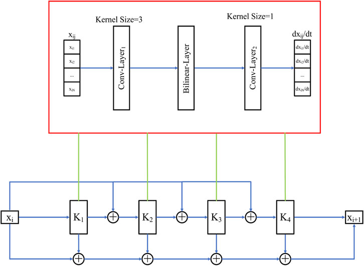
FIGURE 1. The structure diagram of the FM-BNN.

2.2 4DVar-ML

Based on 4DVar, this study establishes a 4DVar-ML assimilation system, where the cost function of 4DVar is shown in Eq. 5:

$\begin{array}{cc}\hfill J\left({\mathbf{x}}_0\right)& =J_b+J_o\hfill \\ \hfill & =\frac{1}{2}{\left({\mathbf{x}}_0-{\mathbf{x}}^b\right)}^T{\mathbf{B}}^{-1}\left({\mathbf{x}}_0-{\mathbf{x}}^b\right)\hfill \\ \hfill & +\frac{1}{2}\sum _{i=0}^n{\left[{\mathit{H}}_i\left({\mathit{M}}_i\left({\mathbf{x}}_{\mathbf{0}}\right)\right)-{\mathbf{y}}_i^o\right]}^T{\mathbf{R}}_i^{-1}\left[{\mathit{H}}_i\left({\mathit{M}}_i\left({\mathbf{x}}_{\mathbf{0}}\right)\right)-{\mathbf{y}}_i^o\right]\hfill \end{array}(5)$

In Eq. 5, x₀ represents the initial state, that is, the control variable, x^b represents the background, i indicates the ith moment, y^o represents the observations, M is the forecast model, H represents the observation operator, B represents the background error coefficient variance matrix, and R represents the observation error covariance matrix. Compared with traditional 4DVar, 4DVar-ML replaces the forecast model (M) based on physical laws with the FM-BNN $(\widehat{\mathit{M}})$ and applies the tangent linear and adjoint models of the FM-BNN to 4DVar. The tangent linear and adjoint models are two parts, one part is the tangent linear model, and the other part is the adjoint model. A tangent linear model (TLM) is a forward model consisting of a series of tangent linear equations to reflect the variation of perturbations with time. The adjoint model is a backward model composed of adjoint equations, and its primary purpose is to calculate gradients (Geer, 2013). Since it is difficult to develop and maintain the tangent linear and adjoint models of the forecast models (Houtekamer and Zhang, 2016), we replace the tangent linear and adjoint models of the physical forecast models in 4DVar with the tangent linear and adjoint models of the FM-BNN. The tangent linear and adjoint models of the FM-BNN are implemented through backpropagation in ML. Previous studies have proven that the adjoint model in 4DVar are equivalent to backpropagation in ML (Geer, 2021).

2.3 EnKF-ML

Similar to 4DVar-ML, we build an EnKF-ML assimilation system. To compare EnKF-ML with traditional EnKF, we introduce the EnKF technique. EnKF was developed based on the Kalman filter (KF). KF is a filtering method based on stochastic process state theory, which includes two steps: forecast and analysis. The specific form of KF is shown in Eqs 6, 7:

• Forecast

$\begin{array}{cc}\hfill {\mathbf{x}}_i^f& ={\mathbf{M}}_{i-1}\left[{\mathbf{x}}_{i-1}^a\right]\hfill \\ \hfill {\mathbf{P}}_i^f& ={\mathbf{M}}_{i-1}{\mathbf{P}}_{i-1}^a{\mathbf{M}}_{i-1}^T+{\mathbf{Q}}_i\hfill \end{array}(6)$

• Analysis

$\begin{array}{cc}\hfill {\mathbf{x}}_i^a& ={\mathbf{x}}_i^f+{\mathbf{K}}_i\left({\mathbf{H}}_i\left({\mathbf{M}}_i\left({\mathbf{x}}_{\mathbf{0}}\right)\right)-{\mathbf{y}}_i^o\right)\hfill \\ \hfill {\mathbf{K}}_i& ={\mathbf{P}}_i^f{\mathbf{H}}_i^T{\left({\mathbf{H}}_i{\mathbf{P}}_i^f{\mathbf{H}}_i^T+{\mathbf{R}}_i\right)}^{-1}\hfill \\ \hfill {\mathbf{P}}_i^a& =\left(\mathbf{I}-{\mathbf{K}}_i{\mathbf{H}}_i^T\right){\mathbf{P}}_i^f\hfill \end{array}(7)$

Where x^f represents the forecast, x^a represents the analysis, Q represents the model error covariance matrix, M is the linear forecast model, H represents the linear observation operator, P^f is the forecast error covariance matrix, P^a represents the analysis error covariance matrix, and K is the Kalman gain matrix.

To lower the computational cost, Evensen et al. combined the ensemble prediction idea with the KF method to obtain the ensemble Kalman filter (EnKF) (Evensen, 1994). To improve the accuracy of analyzing the error covariance, we add a perturbation whose error follows a Gaussian distribution to the observation vector at each analysis time and obtain an ensemble of observations with the same number of members as the ensemble (Houtekamer and Mitchell, 1998). EnKF makes use of the ensemble method to estimate P^f, and its specific form is shown in Eq. 8:

$\begin{array}{cc}\hfill {\mathbf{P}}_i^f& =\frac{1}{m-1}\sum _{l=1}^m\left({\mathbf{x}}_l^f-\overline{{\mathbf{x}}^f}\right){\left({\mathbf{x}}_l^f-\overline{{\mathbf{x}}^f}\right)}^T\hfill \\ \hfill \overline{{\mathbf{x}}^f}& =\frac{1}{m}\sum _{l=1}^m{\mathbf{x}}_l^f\hfill \end{array}(8)$

where $\overline{{\mathbf{x}}^f}$ represents the mean of the ensemble forecast results and m represents the number of ensemble members. In EnKF-ML, we use the FM-BNN as a substitute for the forecast model based on physical laws.

2.4 HDA-ML

In the hybrid DA, we need to combine 4DVar and EnKF using empirical coefficients, reducing the accuracy of the assimilation results. This study utilizes a ML model to couple the analysis of 4DVar and EnKF to improve the accuracy of the assimilation results. In this process, 2 vectors are processed into 1 vector in a specific way, which can be regarded as dimensionality reduction. Many studies have shown that CNN models can be applied for dimensionality reduction tasks and achieve excellent results (Cascianelli et al., 2018; Gao et al., 2019; Zebari et al., 2020). We use a CNN model to replace the empirical coefficients in hybrid DA in the above context. The structure of the CNN model is shown in Figure 2, where x^var represents the assimilation result of Var DA, and x^ens represents the assimilation result of ensemble DA. The CNN model consists of 5 convolutional layers with kernels of sizes 5 and 3. The structure of this CNN model is the same in different applications.

FIGURE 2

FIGURE 2. The structure diagram of the CNN.

This paper employs PyTorch to build the FM-BNN and the CNN and uses the mean squared error (MSE) as the loss function during the training process. We need to train the FM-BNN. Its cost function is shown in Eq. 9:

${\mathcal{L}}_{\widehat{\mathit{M}}}\left(W\right)=\Vert {\mathbf{x}}_{i+1}-\widehat{\mathit{M}}\left({\mathbf{x}}_i\right){\Vert }_2(9)$

where W represents the parameters of the FM-BNN and ‖ ⋅‖₂ represents the 2-norm. We also need to train the CNN model. To test the feasibility of the CNN model, we utilize the true x^t as the label for training. After the test, we choose the observations y^o as the labels for greater realism. Therefore, we use two labels, the true x^t and the observations y^o, and their cost functions are shown in Eqs 10, 11:

${\mathcal{L}}_{\mathbf{CNN}}\left(W\right)=\Vert {\mathbf{x}}^t-\mathbf{C}\mathbf{N}\mathbf{N}\left({\mathbf{x}}_{\mathit{var}}^a,{\mathbf{x}}_{\mathit{ens}}^a\right){\Vert }_2(10)$

${\mathcal{L}}_{\mathbf{CNN}}\left(W\right)={\left[\mathit{H}\left(\mathbf{C}\mathbf{N}\mathbf{N}\left({\mathbf{x}}_{\mathit{var}}^a,{\mathbf{x}}_{\mathit{ens}}^a\right)\right)-{\mathbf{y}}^o\right]}^T{\mathbf{R}}^{-1}\left[\mathit{H}\left(\mathbf{C}\mathbf{N}\mathbf{N}\left({\mathbf{x}}_{\mathit{var}}^a,{\mathbf{x}}_{\mathit{ens}}^a\right)\right)-{\mathbf{y}}^o\right](11)$

where ${\mathbf{x}}_{\mathit{var}}^a$ represents the analysis of 4DVar-ML, ${\mathbf{x}}_{\mathit{ens}}^a$ represents the ensemble analysis mean of EnKF-ML, R stands for the observation error covariance matrix and H represents the observation operator.

After obtaining the FM-BNN and the CNN, we build a hybrid DA based on ML (HDA-ML). The structure of HDA-ML is shown in Figure 3. HDA-ML consists of two main parts. The first part is the assimilation module, which is used to assimilate the background x^b and the observations y^o to obtain the analysis x^a; the second is the forecast module, which predicts the state at the next moment.

FIGURE 3

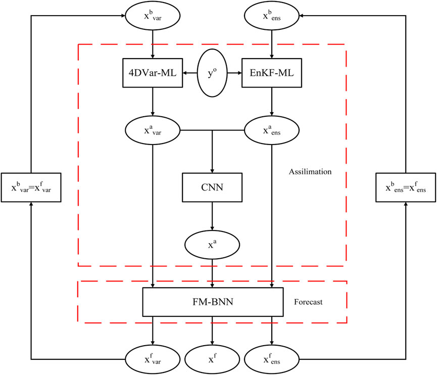
FIGURE 3. The structure diagram of HDA-ML.

The specific process of HDA-ML is as follows:

1) At the ith time, we take the forecasts ${\mathbf{x}}_{\mathit{var}}^b$ and ${\mathbf{x}}_{\mathit{ens}}^b$ of the i − 1st time as the background and input them into the assimilation system. ${\mathbf{x}}_{\mathit{var}}^b$ is input into 4DVar-ML, and ${\mathbf{x}}_{\mathit{var}}^a$ is obtained; ${\mathbf{x}}_{\mathit{ens}}^b$ is input into EnKF-ML, and ${\mathbf{x}}_{\mathit{ens}}^a$ is output after system assimilation.

2) We input ${\mathbf{x}}_{\mathit{var}}^a$ and ${\mathbf{x}}_{\mathit{ens}}^a$ into the CNN, and the final analysis x^a is output.

3) The analysis x^a is employed as the initial field input to the FM-BNN, and the forecast result x^f is obtained; ${\mathbf{x}}_{\mathit{var}}^a$ and ${\mathbf{x}}_{\mathit{ens}}^a$ are also input to the FM-BNN to obtain ${\mathbf{x}}_{\mathit{var}}^f$ and ${\mathbf{x}}_{\mathit{ens}}^f$. Then, ${\mathbf{x}}_{\mathit{var}}^f$ and ${\mathbf{x}}_{\mathit{ens}}^f$ are used as the background at the i + 1st time. Through the analysis cycle of HDA-ML, we can continuously forecast and obtain the state at a future time.

3 Experiments and results

3.1 Experimental setting

3.1.1 The Lorenz-96 model

The numerical prediction system is a compound. It often takes much time to verify a new method in the numerical prediction system, and the workload of modifying the codes in the system is great (Lewis et al., 2006). Thus, we conduct relevant experimental analysis on the Lorenz-96 model. The Lorenz-96 model is a nonlinear system and is often applied to simulate the evolution of atmospheric states over time, so the Lorenz-96 model is widely used in studying DA methods (Whitaker and Hamill, 2002; Nerger, 2015). The definition of the Lorenz-96 model is shown in Eq. 12:

$\frac{d{x}_j}{dt}=\left(x_{j+1}-x_{j-2}\right)x_{j-1}-x_j+F,j=\mathrm{1,2},\dots ,J(12)$

where x_j stands for the state value of the jth grid point, F represents the external forcing parameter, and J represents the number of state variables. The Lorenz-96 adopts cyclic boundary conditions, where x₋₁ = x_J−1, x₀ = x_J, x_J+1 = x₁, J ≥ 4. The Lorenz-96 model includes three terms: the advection term, the dissipation term, and the external forcing term, which are the main features of atmospheric motion. This paper uses J = 40, F = 8, and the fourth-order Runge-Kutta method to integrate Eq. 12 (Brajard et al., 2020; McCabe and Brown, 2021).

3.1.2 Parameter settings for the DA experiments

This paper uses the NMC method to calculate the background error covariance matrix B in Eq. 5, where the calculation formula of the NMC method is shown in Eq. 13. In this paper, the value of α is the maximum value on the diagonal of the covariance matrix. This paper sets the observation error covariance matrix R_i = I and sets the observation operator H_i = I. The length of the assimilation time window is 0.05 MTU. There are 4 observations in an assimilation time window, and the interval of each observation is the same, 0.0125 MTU. The assimilation experiments in this paper are carried out 1,000 times.

$\mathbf{B}\approx \alpha E\left\{\left[{\mathbf{x}}^f\left(48h\right)-{\mathbf{x}}^f\left(24h\right)\right]{\left[{\mathbf{x}}^f\left(48h\right)-{\mathbf{x}}^f\left(24h\right)\right]}^T\right\}(13)$

3.1.3 Data preparation

The true x^t of each experiment is given randomly, and the observations y^o are obtained by adding a disturbance to the true, where the disturbance has a Gaussian distribution with variance 1 and mean 0, as shown in Eq. 14.

$\begin{array}{cc}\hfill {\mathbf{y}}^o& ={\mathbf{x}}^t+\sigma \hfill \\ \hfill \sigma & \sim \mathcal{N}\left(\mathrm{0,1}\right)\hfill \end{array}(14)$

3.1.4 Evaluation indicators

We aim to contrast different assimilation systems and then conduct a systematic and comprehensive evaluation of their assimilation and forecast capabilities, which requires the selection of evaluation indicators. Considering (Ji et al., 2015), we choose the RMSE and R² to assess the assimilation system, and their formulas are shown in Eq. 16:

$\text{RMSE}={\left[\frac{1}{J}\sum _{j=1}^J{\left(x_j-y_j\right)}^2\right]}^{1/2}(15)$

${\text{R}}^2={\left[\frac{{\sum }_{j=1}^J\left(x_j-\bar{x}\right)\left(y_j-\bar{y}\right)}{\sqrt{{\sum }_{j=1}^J{\left(x_j-\bar{x}\right)}^2}\sqrt{{\sum }_{j=1}^J{\left(y_k-\bar{y}\right)}^2}}\right]}^2(16)$

Where x_j and y_j represent the state values on the jth grid point, $\bar{x}$ represents the average value of x, $\bar{y}$ is the average value of y and J represents the total number of grid points. The RMSE reflects the overall error of the system. The value range is $\left[0,+\infty \right)$. The smaller the value is, the smaller the error of the predicted value and the better the model’s performance. R² represents the fitting ability of the model. The value range is [0, 1]. The closer the value is to 1, the stronger the fitting ability of the model is.

3.2 DA experiments

3.2.1 4DVar-ML assimilation experiment

4DVar-ML is applied to construct HDA-ML. Compared with traditional 4DVar, the forecast and tangent linear and adjoint models of 4DVar-ML are derived from the FM-BNN. The experiments below were carried out to compare the assimilation performance of 4DVar-ML and 4DVar. We gave these DA systems the same initial fields, and 1,000 analysis cycles were performed on the observations; then, we calculated the RMSE and R² of x^a. The experimental results are shown in Figure 4. The yellow line indicates 4DVar-ML, and the blue line represents 4DVar. Figure 4A shows the changes in RMSE during assimilation, and Figure 4B indicates the changes in R² during assimilation. As seen in Figure 4, the RMSE of 4DVar-ML is smaller than that of 4DVar, and the R² of 4DVar-ML is greater than that of 4DVar. RMSE and R² are fluctuating. This is because after the spin-up time of the assimilation system, the performance of the assimilation system gradually tends to be stable, and various indicators will change within specific ranges. The experimental results show that the error between the x^a of 4DVar-ML is smaller, and the fitting degree to x^t is higher.

FIGURE 4

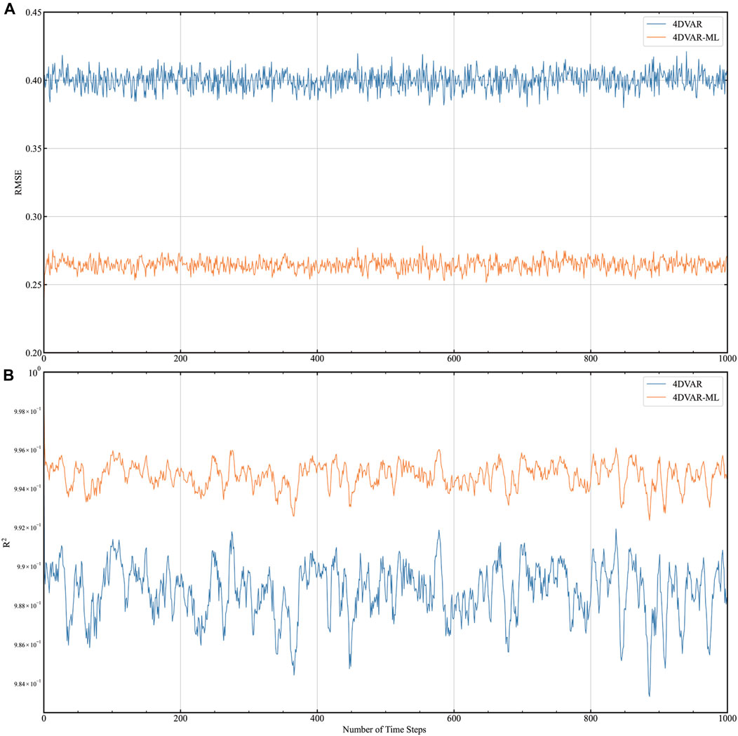
FIGURE 4. Comparison of the RMSE and R² of 4DVar-ML and 4DVar. (A) shows the change in RMSE over time, and (B) depicts the change in R² over time.

To comprehensively and intuitively compare the assimilation performance, forecast quality, and computational efficiency of these DA techniques, we recorded the average RMSE, R², and running time values in Table 1 (bold indicates the best results). Compared with the x^a of 4DVar, the RMSE of 4DVar-ML was reduced by approximately 33.9%, and the R² increased by approximately 6.5%. Compared with the x^f of 4DVar, the RMSE of 4DVar-ML decreased by approximately 31.4%, and the R² increased by approximately 6%. The runtime of 4DVar-ML was approximately 71.2% lower than that of 4DVar. The experimental results show that the assimilation performance, forecast quality, and computational efficiency of 4DVar-ML are better than those of 4DVar, which also indicates that the FM-BNN and the tangent linear and adjoint models of the FM-BNN play a positive role in the assimilation effect.

TABLE 1

TABLE 1. The assimilation performance, forecast quality and computational efficiency of 4DAVar-ML and 4DVar.

3.2.2 EnKF-ML assimilation experiment

The assimilation performance and computational efficiency of the EnKF are related to the number of ensemble members, so we should study and analyse the effect of the number of ensemble members on the assimilation performance and computational efficiency. Figure 5 shows the variation in RMSE and running time with the number of ensemble members. The solid blue line represents the RMSE, and the solid yellow line represents the runtime. Figure 5 shows that as the number of ensemble members increases, the RMSE decreases and the running time increases.

FIGURE 5

FIGURE 5. Variation in the RMSE and running time with the number of ensemble members. (A) shows the variation of RMSE with the number of ensemble members, (B) depicts the variation of the running time with the number of ensemble members.

The RMSE, the running time, and their rates of change are recorded in Table 2, where $\frac{\text{dRMSE}}{\text{dN}}$ indicates the amount of change in the RMSE when adding a collection member and $\frac{\text{dt}}{\text{dN}}$ is the amount of change in the running time when adding a collection member. As shown in Table 2, as the number of ensemble members increases, the RMSE decreases, and the running time changes less. When the ensemble membership grew from 10 to 20, the RMSE decreased by approximately 0.02, which was the most significant decrease in RMSE. Considering the computational cost and assimilation quality comprehensively, we set the number of ensemble members to 20.

TABLE 2

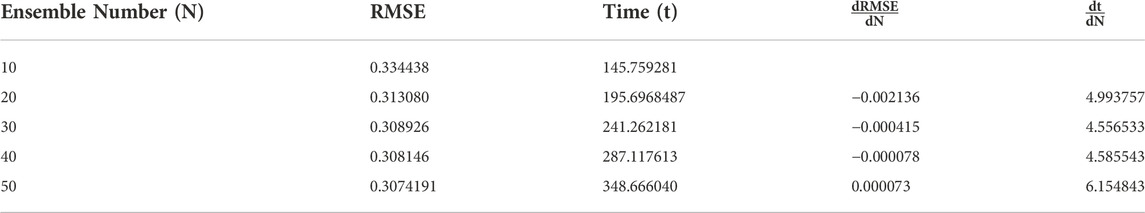
TABLE 2. The assimilation performance and time cost with the number of ensemble members.

We conducted comparative experiments on EnKF-ML and EnKF, and the results are shown in Figure 6. The solid yellow line in this figure represents EnKF-ML, and the blue line represents EnKF. Figure 6A shows changes in the RMSE during assimilation, and Figure 6B shows changes in R² during assimilation. It can be seen that the RMSE and R² of the two are relatively close and that both remain steadily within an interval.

FIGURE 6

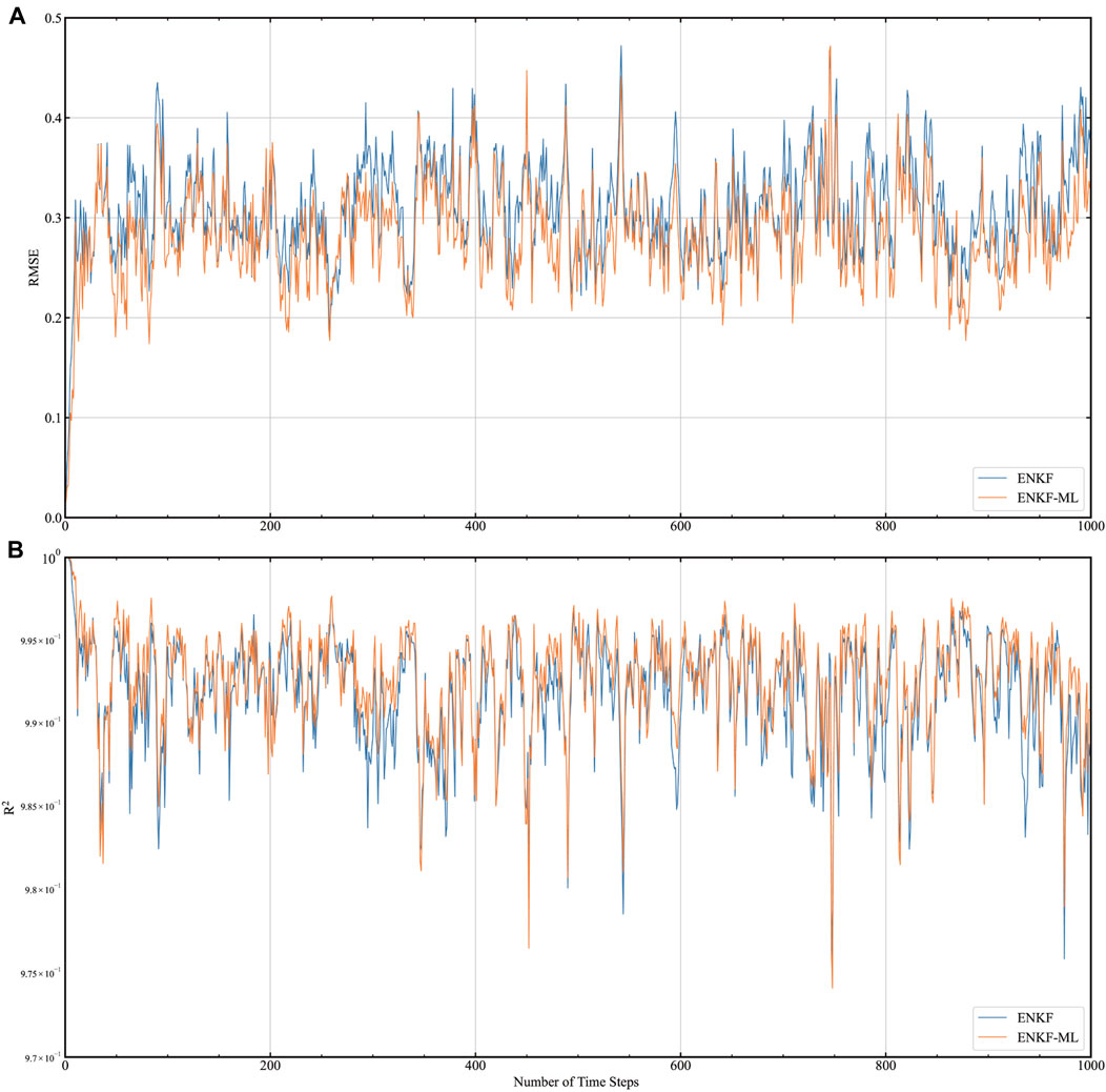
FIGURE 6. Comparison of the RMSE and R² of EnKF-ML and EnKF. (A) shows the change in RMSE over time, and (B) depicts the change in R² over time.

To further compare the assimilation performance, forecast quality, and computational efficiency of EnKF-ML and EnKF, the RMSE, R², and running time are recorded in Table 3. As seen from Table 3, compared with the x^a of EnKF, the RMSE of EnKF-ML is approximately 7.9% lower, and the increase in R² is less than 10⁻⁴. Compared to the forecast of EnKF, the RMSE of EnKF-ML is approximately 8.7% lower, and the increase in R² is less than 10⁻⁴. The running time of EnKF-ML is approximately 38.8% of the running time of EnKF. The above experimental results show that the assimilation performance, forecast quality, and computational efficiency of EnKF-ML are better than those of EnKF.

TABLE 3

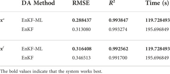
TABLE 3. The assimilation performance, forecast quality and computational efficiency of EnKF-ML and EnKF.

3.2.3 HDA-ML assimilation experiment

We aimed to test the performance of the CNN model. The MLP model is also a standard algorithm that can be used for dimensionality reduction (Omkar et al., 2010), so we compared the properties of the CNN model and the MLP model. We applied the CNN and MLP models to replace the hybrid module in the traditional HDA and then contrasted the accuracy of the results of the two assimilation systems. The results are shown in Table 4. HDA-ML_CNN indicates that the hybrid module is the CNN model, and HDA-ML_MLP means that the hybrid module is the MLP model. It can be seen from the table that the error of x^a of HDA-ML_CNN is smaller, and the fitting ability to x^t is superior. Therefore, we use HDA-ML_CNN as a hybrid module of HDA-ML. HDA-ML is applied instead of HDA-ML_CNN below for brevity.

TABLE 4

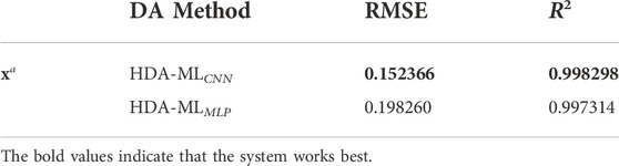
TABLE 4. The assimilation performance of HDA-ML_CNN and HDA-ML_MLP.

Table 5 records the performances of 4DVar-ML, EnKF-ML, and HDA-ML. Table 5 shows that the error between the analysis x^a of HDA-ML and the forecast x^f is the smallest, and the fitting degree with the true x^t is the highest. The experimental results show that the CNN model can play a positive role and improve the accuracy of the assimilation and forecasting results.

TABLE 5

TABLE 5. Comparison of 4DVar-ML, EnKF-ML and HDA-ML

HDA-ML is based on the 4DVar-ML, EnKF-ML, and CNN models. Its forecast model and tangent linear and adjoint models are obtained from the FM-BNN, and its hybrid module makes use of the CNN model to combine the assimilation results of 4DVar-ML and EnKF-ML. We give HDA-ML the same initial fields and observations as HDA to contrast their assimilation performance. We plot the RMSE and R² of the x^a of HDA-ML and HDA during assimilation in Figure 7. The solid yellow line represents HDA-ML, and the solid blue line represents HDA. Figure 7 shows that the variations in the RMSE and R² of the x^a of HDA-ML are smaller than the variations in the RMSE and R² of the x^a of HDA.

FIGURE 7

FIGURE 7. Comparison of the RMSE and R² of HDA-ML and HDA. (A) shows the change in RMSE over time, and (B) depicts the change in R² over time.

Their average RMSE, R², and running time values are recorded in Table 6. In the table, the RMSE of the x^a and x^f of HDA is the largest, the R² is the smallest, and the running time is the longest. Compared with that of the x^a of HDA, the RMSE of the HDA-ML is decreased by approximately 15.9%, and the increase in R² is less than 10⁻⁴. Compared with that of the x^f of HDA, the RMSE of HDA-ML is approximately 21.0% lower, and the increase in R² is less than 10⁻⁴. Compared with the running time of HDA, the running time of HDA-ML is reduced by 26.6%. The experimental results show that the assimilation and forecast results of HDA-ML are more accurate and the computational cost is lower.

TABLE 6

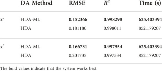
TABLE 6. The assimilation performance, forecast quality and computational efficiency of HDA-ML and HDA.

3.2.4 HDA-ML_o assimilation experiment

Since the true x^t is difficult to obtain in the real world, we should test using observations (The observations are generated as shown in Eq. 14) as dataset labels to train CNN models. On this basis, we established HDA-ML_o. We plot the RMSE and R² of HDA-ML_o for each assimilation moment in Figure 8. The solid blue line represents HDA, and the solid yellow line represents HDA-ML_o. The figure shows that the RMSE of HDA-ML_o varies less than that of HDA.

FIGURE 8

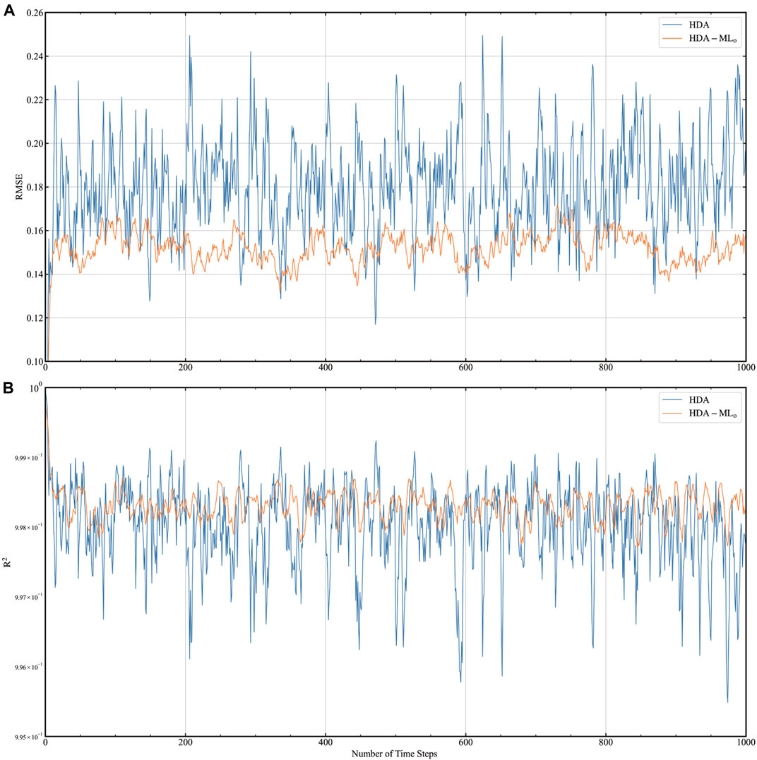
FIGURE 8. Comparison of the RMSE and R² of HDA-ML_o and HDA. (A) shows the change in RMSE over time, and (B) depicts the change in R² over time.

The assimilation performance, prediction quality, and computational cost of HDA-ML_o with respect to HDA are recorded in Table 7. As seen from Table 7, compared with the x^a and x^f of HDA, HDA-ML_o has the smallest RMSE and the largest R². Additionally, the computation time of HDA-ML_o is the shortest. The above experimental results show that the assimilation performance of HDA-ML_o is higher than that of HDA in terms of prediction quality and computational efficiency. The RMSE, R² and computational efficiency of HDA-ML_o and HDA-ML are recorded in Table 7. As seen from Table 7, the difference between the two is minimal. The experimental results show that it is feasible to use observations as labels for training data.

TABLE 7

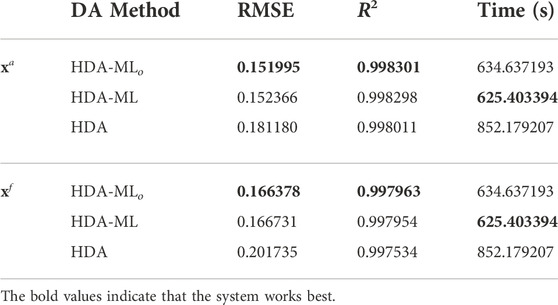
TABLE 7. The assimilation performance, forecast quality and computational efficiency of HDA-ML_o, HDA-ML and HDA.

4 Discussion

In this paper, we replace the prediction model in hybrid DA with FM-BNN and use the tangent linear and adjoint models of FM-BNN in hybrid DA 4DVar. On this basis, we establish 4DVar-ML and EnKF-ML. Then, we combine the analysis of 4DVar-ML with that of EnKF-ML using the CNN model, and in the process, we also train the CNN model with the observations as labels. The results of the discussions of these experiments are as follows:

The FM-BNN can replace the forecast model, while the tangent linear and adjoint models of the FM-BNN can be used to build a 4DVar system. We construct 4DVar-ML and EnKF-ML and compare their performances with those of traditional methods. It can be seen from the experimental results that 4DVar-ML performs better than the conventional 4DVar technique, which indicates that FM-BNN and its tangent linear and adjoint models can play a role in 4DVar. The performance of EnKF-ML is better than that of the traditional EnKF, which shows that using FM-BNN as a prediction model can improve the accuracy of the assimilation results.

The CNN model can also improve the accuracy of the assimilation results. We utilize the CNN model to combine the analysis of both. By comparing the accuracy of 4DVar-ML, EnKF-ML, and HDA-ML, we find that the assimilation performance and prediction quality of HDA-ML are higher than those of 4DVar-ML and EnKF-ML. The experimental results show that the CNN model can enhance the quality of assimilation. In the comparison experiment between HDA-ML and HDA, we can see that the assimilation performance, prediction quality, and computational efficiency of HDA-ML are greatly improved.

Observations can be used as labels to train a CNN model. When training the CNN model, we changed the labels to the observations to better simulate real-world scenarios. It can be seen from the experimental results that the performance of HDA-ML_o is very close to that of HDA-ML and is superior to that of HDA. The experimental results show that using the observations as training labels is feasible.

The related experiments in this paper are carried out on the Lorenz-96 model. Compared to the real atmospheric model, the Lorenz-96 model is simple. Therefore, if we use the ML model to simulate the real atmospheric model, we need to build a complex, suitable network model. These experiments require adequate hardware support. At the same time, most current models are written in Fortran, while many ML codes are written in Python. Coupling Fortran programs with Python programs is a problem to be solved in the future.

5 Conclusion

To simplify the development and maintenance of tangent linear and adjoint models in hybrid data assimilation (HDA) and decrease the errors introduced by artificially chosen hybrid coefficients, we create a hybrid data assimilation method based on ML (HDA-ML). We apply a forecast model based on a bilinear neural network (FM-BNN) to replace the physical forecast model in HDA. The tangent linear and adjoint models of the FM-BNN are employed in 4DVar to build 4DVar-ML. Additionally, we combine the FM-BNN with the EnKF to form EnKF-ML. Then, we use the CNN model to couple the x^a of 4DVar-ML and EnKF-ML. On this basis, we establish HDA-ML. The experimental results show that HDA-ML improves the assimilation result accuracy, enhances the prediction result quality, and reduces the running time.

With the improvement of ML theory, the increase in data volume, the development of computer hardware, and the reduction in the cost of developing ML models, the application scope of ML has become increasingly extensive, and ML can achieve excellent results in some challenging cases. Two primary purposes of using ML in NWP are to improve the model’s prediction accuracy and reduce the model’s computational cost. We conducted related experiments on the Lorenz-96 model. The experiments show the reliability of the ML model and its tangent linear and adjoint models and prove that the ML model can be applied to HDA. In the future, we can design an HDA-ML that can be used for an actual model to facilitate the development of NWP.

Data availability statement

The raw data supporting the conclusion of this article will be made available by the authors, without undue reservation.

Author contributions

CZ provided the research ideas of this paper, and RD and HL carried out related experiments. JS polished the language and pictures in the paper. JZ and XC are responsible for the editing and review of the paper.

Funding

This work is supported by the National Natural Science Foundation of China (Grant No. 41605070) and the National Key R&D Program of China (Grant No. 2018YFC1506704).

Conflict of interest

The authors declare that the research was conducted in the absence of any commercial or financial relationships that could be construed as a potential conflict of interest.

Publisher’s note

All claims expressed in this article are solely those of the authors and do not necessarily represent those of their affiliated organizations, or those of the publisher, the editors and the reviewers. Any product that may be evaluated in this article, or claim that may be made by its manufacturer, is not guaranteed or endorsed by the publisher.

References

Atkinson, K., Han, W., and Stewart, D. E. (2011). Numerical solution of ordinary differential equations. John Wiley & Sons.

Google Scholar

Bannister, R. (2017). A review of operational methods of variational and ensemble-variational data assimilation. Q. J. R. Meteorol. Soc. 143, 607–633. doi:10.1002/qj.2982

CrossRef Full Text | Google Scholar

Bauer, P., Thorpe, A., and Brunet, G. (2015). The quiet revolution of numerical weather prediction. Nature 525, 47–55. doi:10.1038/nature14956

PubMed Abstract | CrossRef Full Text | Google Scholar

Bjerknes, V. (1904). Das problem der wettervorhers-age, betrachtet vom standpunkte der mechanik und der physik. Meteor. Z. 21, 1–7.

Google Scholar

Bowler, N. E., Arribas, A., Mylne, K. R., Robertson, K. B., and Beare, S. E. (2008). The mogreps short-range ensemble prediction system. Q. J. R. Meteorol. Soc. 134, 703–722. doi:10.1002/qj.234

CrossRef Full Text | Google Scholar

Brajard, J., Carrassi, A., Bocquet, M., and Bertino, L. (2020). Combining data assimilation and machine learning to emulate a dynamical model from sparse and noisy observations: A case study with the lorenz 96 model. J. Comput. Sci. 44, 101171. doi:10.1016/j.jocs.2020.101171

CrossRef Full Text | Google Scholar

Carrassi, A., Bocquet, M., Bertino, L., and Evensen, G. (2018). Data assimilation in the geosciences: An overview of methods, issues, and perspectives. WIREs Clim. Change 9, e535. doi:10.1002/wcc.535

CrossRef Full Text | Google Scholar

Cascianelli, S., Bello-Cerezo, R., Bianconi, F., Fravolini, M. L., Belal, M., Palumbo, B., et al. (2018). “Dimensionality reduction strategies for cnn-based classification of histopathological images,” in International conference on intelligent interactive multimedia systems and services (Springer), 21–30.

CrossRef Full Text | Google Scholar

Chen, R. T., Rubanova, Y., Bettencourt, J., and Duvenaud, D. K. (2018). Neural ordinary differential equations. Adv. neural Inf. Process. Syst. 31, 1.

Google Scholar

[Dataset] Krasnopolsky, V. (2002). Using machine learning for model physics: An overview. Ithaca, NY: arxiv.

Google Scholar

Demirtas, M., Barker, D., Chen, Y., Hacker, J., Huang, X.-Y., Snyder, C., et al. (2009). A hybrid data assimilation (wrf-var and ensemble transform kalman filter) system based retrospective tests. Available at: http://www.mmm.ucar.edu/wrf/users/workshops/WS2009/abstracts/2A-10.pdf.

Google Scholar

Dong, R., Leng, H., Zhao, J., Song, J., and Liang, S. (2022). A framework for four-dimensional variational data assimilation based on machine learning. Entropy 24, 264. doi:10.3390/e24020264

PubMed Abstract | CrossRef Full Text | Google Scholar

Dueben, P., Modigliani, U., Geer, A., Siemen, S., Pappenberger, F., Bauer, P., et al. (2021). Technical memo. Reading, UK: European Centre for Medium-Range Weather Forecasts.

Google Scholar

Evensen, G. (1994). Sequential data assimilation with a nonlinear quasi-geostrophic model using Monte Carlo methods to forecast error statistics. J. Geophys. Res. 99, 10143–10162. doi:10.1029/94jc00572

CrossRef Full Text | Google Scholar

Fablet, R., Ouala, S., and Herzet, C. (2018). “Bilinear residual neural network for the identification and forecasting of geophysical dynamics,” in 2018 26th European signal processing conference (EUSIPCO) (IEEE), 1477–1481.

CrossRef Full Text | Google Scholar

Fan, M., Bai, Y., Wang, L., and Ding, L. (2021). Combining a fully connected neural network with an ensemble kalman filter to emulate a dynamic model in data assimilation. IEEE Access 9, 144952–144964. doi:10.1109/access.2021.3120482

CrossRef Full Text | Google Scholar

Frerix, T., Kochkov, D., Smith, J., Cremers, D., Brenner, M., and Hoyer, S. (2021). “Variational data assimilation with a learned inverse observation operator,” in International conference on machine learning (PMLR) (IEEE), 3449–3458.

Google Scholar

Gao, Y., Ma, J., Zhao, M., Liu, W., and Yuille, A. L. (2019). “Nddr-cnn: Layerwise feature fusing in multi-task cnns by neural discriminative dimensionality reduction,” in Proceedings of the IEEE/CVF conference on computer vision and pattern recognition (IEEE), 3205–3214.

CrossRef Full Text | Google Scholar

Geer, A. (2021). Learning Earth system models from observations: Machine learning or data assimilation? Philos. Trans. A Math. Phys. Eng. Sci. 379, 20200089. doi:10.1098/rsta.2020.0089

PubMed Abstract | CrossRef Full Text | Google Scholar

Geer, I. W. (2013). Glossary of weather and climate. Bull. Am. Meteorological Soc. 94, 1936–1937.

Google Scholar

Gettelman, A., Geer, A. J., Forbes, R. M., Carmichael, G. R., Feingold, G., Posselt, D. J., et al. (2022). The future of Earth system prediction: Advances in model-data fusion. Sci. Adv. 8, eabn3488. doi:10.1126/sciadv.abn3488

PubMed Abstract | CrossRef Full Text | Google Scholar

Haltiner, G. J., and Williams, R. T. (1980). Numerical prediction and dynamic meteorology. Manhattan: Tech. rep.

Google Scholar

Houtekamer, P. L., and Mitchell, H. L. (1998). Data assimilation using an ensemble kalman filter technique. Mon. Weather Rev. 126, 796–811. doi:10.1175/1520-0493(1998)126<0796:dauaek>2.0.co;2

CrossRef Full Text | Google Scholar

Houtekamer, P. L., and Zhang, F. (2016). Review of the ensemble kalman filter for atmospheric data assimilation. Mon. Weather Rev. 144, 4489–4532. doi:10.1175/mwr-d-15-0440.1

CrossRef Full Text | Google Scholar

Ixaru, L. G. (1984). Numerical methods for differential equations and applications. Springer.

Google Scholar

Ji, L., Senay, G. B., and Verdin, J. P. (2015). Evaluation of the global land data assimilation system (gldas) air temperature data products. J. Hydrometeorol. 16, 2463–2480. doi:10.1175/jhm-d-14-0230.1

CrossRef Full Text | Google Scholar

Lewis, J. M., Lakshmivarahan, S., and Dhall, S. (2006). Dynamic data assimilation: A least squares approach, vol. 13. Cambridge: Cambridge University Press.

Google Scholar

Lu, J., Ren, K., Li, X., Zhao, Y., Xu, Z., and Ren, X. (2022). From reanalysis to satellite observations: Gap-filling with imbalanced learning. GeoInformatica 26, 397–428. doi:10.1007/s10707-020-00426-7

CrossRef Full Text | Google Scholar

McCabe, J., and Brown, J. (2021). Learning to assimilate in chaotic dynamical systems. Adv. Neural Inf. Process. Syst. 34, 12237–12250.

Google Scholar

Nerger, L. (2015). On serial observation processing in localized ensemble kalman filters. Mon. Weather Rev. 143, 1554–1567. doi:10.1175/mwr-d-14-00182.1

CrossRef Full Text | Google Scholar

Omkar, S., Sivaranjani, V., Senthilnath J, J., and Mukherjee, S. (2010). Dimensionality reduction and classification of hyperspectral data. Int. J. Aerosp. Innovations 2, 157–164. doi:10.1260/1757-2258.2.3.157

CrossRef Full Text | Google Scholar

Rabier, F., Järvinen, H., Klinker, E., Mahfouf, J.-F., and Simmons, A. (2000). The ecmwf operational implementation of four-dimensional variational assimilation. i: Experimental results with simplified physics. Q. J. R. Meteorol. Soc. 126, 1143–1170. doi:10.1002/qj.49712656415

CrossRef Full Text | Google Scholar

Rasp, S., and Lerch, S. (2018). Neural networks for postprocessing ensemble weather forecasts. Mon. Weather Rev. 146, 3885–3900. doi:10.1175/mwr-d-18-0187.1

CrossRef Full Text | Google Scholar

Song, H.-J., and Roh, S. (2021). Improved weather forecasting using neural network emulation for radiation parameterization. J. Adv. Model. Earth Syst. 13, e2021MS002609. doi:10.1029/2021ms002609

CrossRef Full Text | Google Scholar

Vapnik, V. N. (2019). Complete statistical theory of learning. Autom. Remote Control 80, 1949–1975. doi:10.1134/s000511791911002x

CrossRef Full Text | Google Scholar

Whitaker, J. S., and Hamill, T. M. (2002). Ensemble data assimilation without perturbed observations. Mon. Weather Rev. 130, 1913–1924. doi:10.1175/1520-0493(2002)130<1913:edawpo>2.0.co;2

CrossRef Full Text | Google Scholar

Yuval, J., and O’Gorman, P. A. (2020). Stable machine-learning parameterization of subgrid processes for climate modeling at a range of resolutions. Nat. Commun. 11 (1), 1–10. doi:10.1038/s41467-020-17142-3

PubMed Abstract | CrossRef Full Text | Google Scholar

Zebari, R., Abdulazeez, A., Zeebaree, D., Zebari, D., and Saeed, J. (2020). A comprehensive review of dimensionality reduction techniques for feature selection and feature extraction. J. Appl. Sci. Technol. Trends 1, 56–70. doi:10.38094/jastt1224

CrossRef Full Text | Google Scholar