Quantification of gas, ash, and sulphate aerosols in volcanic plumes from open path Fourier transform infrared (OP-FTIR) emission measurements at Stromboli volcano, Italy

Field-portable Open Path Fourier Transform Infrared (OP-FTIR) spectrometers can be used to remotely measure the composition of volcanic plumes using absorption spectroscopy, providing invaluable data on total gas emissions. Quantifying the temporal evolution of gas compositions during an eruption helps develop models of volcanic processes and aids in eruption forecasting. Absorption measurements require a viewing geometry which aligns infrared source, plume, and instrument, which can be challenging. Here, we present a fast retrieval algorithm to estimate quantities of gas, ash and sulphate aerosols from thermal emission OP-FTIR measurements, and the results from two pilot campaigns on Stromboli volcano in Italy in 2019 and 2021. We validate the method by comparing time series of SO₂ slant column densities retrieved using our method with those obtained from a conventional UV spectrometer, demonstrating that the two methods generally agree to within a factor of 2. The algorithm correctly identifies ash-rich plumes and gas bursts associated with explosions and quantifies the mass column densities and particle sizes of ash and sulphate aerosols (SA) in the plume. We compare the ash sizes retrieved using our method with the particle size distribution (PSD) of an ash sample collected during the period of measurements in 2019 by flying a Remotely Piloted Aircraft System into the path of a drifting ash plume and find that both modes of the bimodal PSD (a fine fraction with diameter around 5–10 μm and a coarse fraction around 65 μm) are identified within our datasets at different times. We measure a decrease in the retrieved ash particle size with distance downwind, consistent with settling of larger particles, which we also observed visually. We measure a decrease in the SO₂/SA ratio as the plume travels downwind, coupled with an increase in measured SA particle size (range 2–6 μm), suggesting rapid hygroscopic particle growth and/or SO₂ oxidation. We propose that infrared emission spectroscopy can be used to examine physical and chemical changes during plume transport and opens the possibility of remote night-time monitoring of volcanic plume emissions. These ground-based analyses may also aid the refinement of satellite-based aerosol retrievals.

1 Introduction

Emissions of gas and particulate matter accompany volcanic activity of all types, from mild effusive eruptions to large explosions. They form volcanic plumes consisting of a mixture of gases and particulates, including sulphate aerosols (SA) and sometimes volcanic ash (Carey and Bursik, 2015), which interact with the atmosphere as they travel away from their source, affecting the environment locally, and sometimes regionally or globally (Delmelle, 2003; Mather, 2015). Depending on the intensity of the emissions, the duration of a particular eruptive episode and the injection height, volcanic emissions can present significant hazards to local populations (Horwell, 2007; Gudmundsson, 2011; Tang et al., 2020; Carlsen et al., 2021), infrastructures (Barsotti et al., 2010; Wilson et al., 2014) and air traffic (Carn et al., 2009; Schmidt et al., 2014). The emergence of automated, continuous monitoring of volcanic plume composition provides valuable insights into the behaviour of volatiles over the course of volcanic crises and technical advances in instrumentation now offer new possibilities to measure plume composition in real-time and in a safe manner (Kern et al., 2022). Here we present a new method to measure gas and particle composition in volcanic plumes using an Open Path Fourier Transform Infrared (OP-FTIR) spectrometer collecting passive emission measurements.

FTIR spectroscopy is a powerful tool to identify and quantify atmospheric composition, as a number of trace gases present distinctive rotational and vibrational features at wavelengths from the near-infrared to the far-infrared. Since the emergence of relatively portable OP-FTIR spectrometers, it has been used extensively by the volcanic gas community over the past 30 years (Notsu et al., 1993; Mori et al., 1995; Mori and Notsu, 1997; Oppenheimer et al., 1998a; Francis et al., 1998; Horrocks et al., 1999; Horrocks et al., 2001). The most common method utilizes hot eruptive material (lava flow, lava dome, lava fountains, etc.) as a source of infrared (IR) radiation to measure the absorption features of the emitted gases directly at the source (Burton et al., 2000; Burton et al., 2007; La Spina et al., 2015; Pfeffer et al., 2018). In order to target passive gas plumes, measurements can also be performed by using the Sun or the Moon as the source of radiation, a method known as solar/lunar occultation (Francis et al., 1998; Burton et al., 2001; Duffell et al., 2001; Butz et al., 2017); or, when the plume travels at or passes through, ground-level, using an artificial IR radiation source placed on the other side of the plume from the observer or combined with a mirror to achieve a longer path length (Burton et al., 2000; Vanderkluysen et al., 2014). These methods all rely on the principle of absorption spectroscopy, whereby the variable of interest (i.e., the quantity of a given gas species) is related to the strength of absorption of radiation by said gas, and the gas quantity is retrieved by fitting a modelled spectrum to the measured spectrum (Burton et al., 2000; Burton et al., 2007). While absorption spectroscopy using a hot radiation source (>∼300°C) offers the key advantage of a relatively simple retrieval of the amounts of the most abundant volcanic gases, a specific geometry to align a hot source, the volcanic plume and the instrument is required. This is quite straightforward to achieve when using the Sun as a source of radiation, but the long atmospheric path then precludes quantification of key gases such as CO₂ and H₂O, although near-infrared solar retrievals of volcanic CO₂ have been demonstrated (Butz et al., 2017). OP-FTIR is most useful when there is explosive volcanic activity, as this provides an ample radiation source. In the case of ash-rich eruption columns only the cooler gas on the outside of the plume is measurable, but this is sufficient to produce accurate retrievals of the key gas species. In these conditions in-situ sensors are extremely challenging to use, so OP-FTIR provides the best opportunity for gas quantification. This has been successfully applied to plumes from effusive or fire fountaining activity using incandescent vents and flows as a source of radiation (Allard et al., 2005; Edmonds and Gerlach, 2007; La Spina et al., 2010; La Spina et al., 2015; Allard et al., 2016), or passive emissions using artificial sources (Burton et al., 2000; Vanderkluysen et al., 2014; Sellitto et al., 2019). When using solar/lunar occultation (Burton et al., 2001; Duffell et al., 2001; Butz et al., 2017), available time windows for measurements are also constrained by the position of the celestial objects in the sky. OP-FTIR is generally used for short regular measurements, where data are collected for a few minutes, rather than for continuous monitoring. One example of continuous monitoring is the Cerberus instrument on Stromboli volcano in Italy (La Spina et al., 2013), a system using hot rocks from the crater walls as a source of IR radiation and capable of determining gas composition from individual vents, which operated between 2009 and 2019 when it was destroyed by a paroxysm episode. Long-term regular (∼weekly) solar FTIR measurements of SO₂, HCl and HF have been conducted on Mt Etna in Italy, and regular daytime measurements of the plume of Popocatépetl volcano in Mexico have been conducted for 4 years (Taquet et al., 2019) using a solar-tracking OP-FTIR instrument originally meant for long-term atmospheric composition monitoring, and which intersected the passive emissions generated by the nearby volcano when the wind direction was favourable.

In contrast, emission spectroscopy quantifies the radiance produced by volcanic gases when viewed against a cold background (i.e., a clear sky or clouds at higher altitudes). The method was first introduced to volcanology by Love et al. (1998), and used to quantify volcanic gases in the gas plume produced by Popocatépetl volcano in Mexico (Love et al., 1998; Love et al., 2000; Goff et al., 2001). The main assumption of the method is of a thermal contrast between a cold sky and a relatively warmer plume. It is therefore best suited for plumes measured close to their emission source (where they are more likely to be warmer than the background atmosphere) and with a relatively high viewing angle, both of which are factors maximizing the thermal contrast. Following these early efforts, the method had been largely unused until more recent studies, once again at Popocatépetl, demonstrated its use for routine measurements of a passive plume (Stremme et al., 2012; Taquet et al., 2017). These most recent efforts focus exclusively on gases, using individual, relatively narrow retrieval windows dedicated to each target gas. When using absorption spectroscopy, the strength of absorption for various gases is quantified by reproducing the observed unprocessed intensity signal (i.e., without performing radiometric calibration), with a model in which the source intensity is simulated by a polynomial function that represents a series of physical parameters, including the Planck function for the source temperature, the instrument response function and, crucially, the broadband absorption of light by particulate species. Similarly, in previous emission studies (Love et al., 1998; Love et al., 2000; Goff et al., 2001; Stremme et al., 2012; Taquet et al., 2017), particulate species which are likely often present in the volcanic plume are treated as interfering with the retrieval and require a correction during data processing or are dismissed during quality control. However, the radiometric calibration performed during the pre-processing stage of emission measurements provides a way of characterizing most of the physical parameters which form the polynomial function described above, and therefore presents a unique opportunity to isolate and quantify the contribution from species with broader spectral features, such as sulphate aerosols and ash. Sellitto et al. (2019) have shown that the simultaneous retrieval of SO₂ and sulphate aerosols is possible from active absorption measurements where the intensity of the radiative source can be assumed to remain constant. They show that the presence of sulphate aerosols may lead to significant overestimation in SO₂ amounts if not accounted for. Accurate quantification of particulate matter (PM) concentration and size in plumes is also important in its own right when forecasting, for example, the respiratory hazards and environmental consequences associated with volcanic emissions (e.g., Ilyinskaya et al., 2017).

In this study we present a fast retrieval algorithm capable of simultaneously extracting slant column densities (SCDs) of gas and particles from OP-FTIR data collected in emission mode in near real-time, using a broad fitting window.

2 Methods

2.1 Data acquisition strategy

We present data from two separate measurement campaigns at Stromboli volcano in Italy: September 9–11, 2019, and September 23–25, 2021 (Figure 1). Thermal emission measurements were performed using a Bruker EM27 OP-FTIR spectrometer lent by the Osservatorio Etneo dell’Istituto Nazionale di Geofisica e Vulcanologia (INGV). The EM27 consists of a “Rock Solid interferometer” (corner cube mirrors on a pendulum around the beam splitter) directing radiation towards a Stirling-cooled Mercury-Cadmium-Telluride (MCT) detector using entirely reflective optics (i.e., no external telescope was added) with an optical path difference of 1.8 cm and a field-of view (FOV) of 30 mrad. Spectra were acquired in the frequency range 600—2,000 cm⁻¹ with a resolution of ∼0.5 cm⁻¹ (or a ∼0.25 cm⁻¹ spectral sampling), and averaged with five co-adds, resulting in a sampling interval of 8–10 s. Radiometric calibration was performed using an internal blackbody target with adjustable temperature. Using two blackbody spectra at two different temperatures (typically around 20°C and 40°C), we created an instrument calibration function which can be applied to convert the single beam spectrum to calibrated radiance or brightness temperature. Clear sky spectra were collected by pointing the instrument towards an area of sky outside of the plume while keeping the inclination angle as close to that of the plume measurements as possible. The duration of acquisition periods varied between 30 min and several hours, and calibration and clear sky measurements were performed every hour or so to account for the thermal drift of the instrument and to reflect changing atmospheric conditions. In datasets for which multiple calibration sets were acquired, we account for instrument drift by interpolating the blackbody spectra between the calibration sets, thereby creating a time-dependent calibration function with unique values for each measurement. We also create a similar time-dependent representation of the expected background spectrum by interpolating between clear sky spectra. This is especially important when working with longer datasets or with datasets acquired at the time of local sunrise and sunset, when the thermal profile of the atmosphere changes rapidly.

FIGURE 1

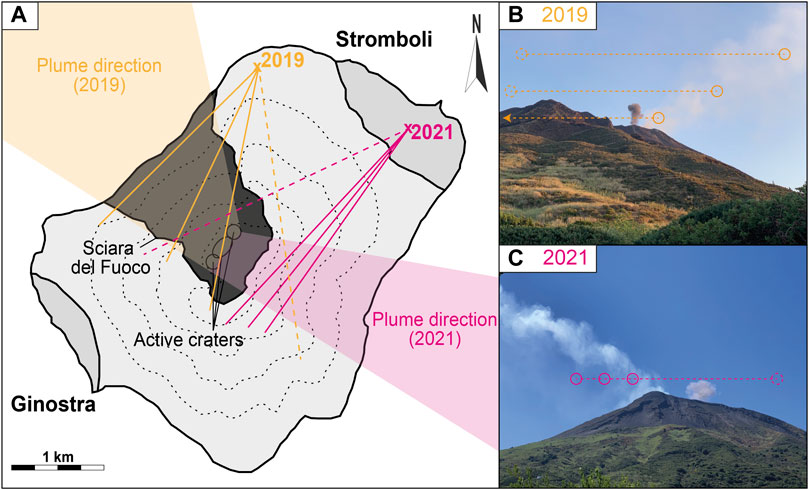
FIGURE 1. (A) Sketch map of the island of Stromboli, depicting the measurement locations and approximate plume geometries during the two measurement campaigns [2019 in yellow, 2021 in magenta]. Grey shaded areas (labeled Stromboli and Ginostra) represent settlements on the island. The black shaded area represents the collapse feature known as the Sciara del Fuoco. The approximate location of the three main crater areas (Northeast, Central and Southwest) is indicated by ellipses. Shaded coloured polygons represent the general plume direction during measurements. Coloured lines represent the range of azimuths during plume (solid) and clear sky (dashed) measurements (B and C) Photographs taken from the measurement location in the 2019 (B) and 2021 (C) campaigns. Circles represent the approximate location of the instrument field of view during plume (solid) and clear sky (dashed) measurements.

During the first field campaign in 2019, measurements were performed from the l’Osservatorio restaurant, providing a direct view of the craters (Figure 1). Wind direction was relatively constant during the 3-day period, and the plume drifted over the Sciara del Fuoco in a NE direction. We collected multiple short sets of 30–60 min of measurements, moving the instrument field-of-view to intersect the plume at various distances from the vent. The activity during this campaign was typical for Stromboli, with explosive events occurring every 5 min on average. Events at the crater were logged manually in a notebook, with the observer entering the time, nature of the event and crater of origin as far as it was possible to observe. We also organized a series of flights with a Remotely Piloted Aircraft System (RPAS) developed and built at the University of Manchester, with the aim of sampling ash from the drifting volcanic plume during the measurement period (Figure 2). The RPAS was a quadcopter carrying a hoover-like sampling mechanism. Once the RPAS had reached the desired location within the plume, the sampling mechanism was triggered remotely, turning on a high mass-flow ducted fan to direct airflow and ash into a small vacuum cleaner bag connected to the system. We were able to collect a single sample at 17:02 local time on 11 September 2019 (analysis results in Section 3.1). The particle size distribution (PSD) of the sample collected during the RPAS flight was measured using a Retch Camsizer X2 particle size analyser at the University of Leeds. Further, the sample was mounted onto SEM stubs using clear epoxy, polished and carbon-coated for analysis with an Electron Microprobe Analyser (EMPA) at the University of Oxford, to determine the chemical composition of individual phases.

FIGURE 2

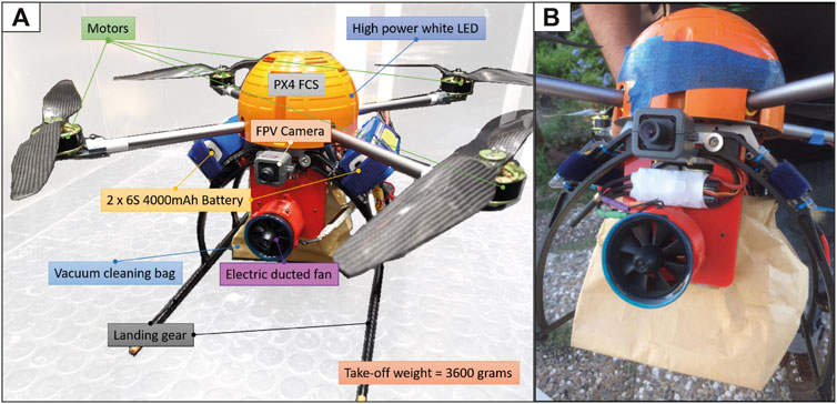
FIGURE 2. (A) Photograph of the Remotely Piloted Aircraft System (RPAS) used during field deployment. The red 3D printed housing seen in the middle of the multirotor houses an electric ducted fan system used to pull air and ash into the sample bag. Acronyms: LED—Light-Emitting Diode; FPV—First-Person View; FCS—Flight Controller System (B) Photograph of the RPAS after successful collection at Stromboli on 11 September 2019. Note the ash particles collected on a piece of tape affixed to the FCS housing in order to confirm plume intercept.

In 2021, measurements were performed from the roof of the Pedra Residence hotel in Stromboli village. The wind direction was approximately to the East, and the line of sight of the instrument intersected the plume as it passed over the summit of the island. We collected longer datasets (3-4 h) with the specific purpose of evaluating the usefulness of the method as a monitoring tool. A GoPro camera was used to capture time-lapse imagery from the observer’s vantage point, and the eruptive events were logged by reviewing the footage. Although the method allows for a continuous record of events over long periods, weaker events and those without an associated ash-rich plume were often not detectable in the footage because we did not have a direct view of the craters. Therefore, we could not assign a specific vent to any given event either. During this second campaign, we also collected simultaneous spectra with a UV spectrometer to validate the infrared SO₂ retrieval. Light was collected using a collimated telescope (diameter = 25.4 mm, f = 100 mm), connected to an Ocean Optics USB 2000+ spectrometer via an optical fibre. The spectrometer was controlled and powered by a connected laptop via USB cable. SO₂ slant column densities were retrieved using the iFit method (Esse et al., 2020). The wavelength window for the retrieval was 310—320 nm and the fit included absorption cross-sections for SO₂ at 295 K (Rufus et al., 2003) and O₃ at 223 K (Serdyuchenko et al., 2014), a Ring spectrum, a wavelength shift and stretch and a linear intensity offset. The instrument line shape (ILS) was characterised using a super-Gaussian with the shape parameters also fitted for each spectrum to account for changes with time (e.g., due to changes in temperature).

2.2 Retrieval algorithm

The emission spectrum retrieval algorithm (developed in Python and available at https://www.github.com/jfsmekens/plumeIR) follows the basic principles laid out by Love et al. (1998), where the simplified radiative transfer expression comprises three layers (Figure 3): 1) a lower layer between the observer and the plume, 2) a plume layer, and 3) an upper layer encompassing the atmosphere in the line-of-sight behind the plume. Given a plume height (h) and a vertical plume thickness (z_v), the plume layer is defined between the height $h_1=h-z_v/2$ and $h_2=h+z_v/2$. The forward model computes the radiance difference between a clear sky and a plume measurement, which offers the advantage of isolating the spectral features of the volcanic species. The aim is to provide a tool which can be used in the field to quantify target species in real time as the measurements are taken (i.e., with a target processing time of <10 s for each individual spectrum, comparable to the acquisition time between consecutive spectra). The algorithm was developed around an iterative non-linear least-squares fitting method. High-resolution radiative transfer calculations (.04 cm⁻¹ spectral sampling) over the entire vertical atmospheric profile are performed in a pre-processing stage to generate reference spectra used in the forward model. In contrast to recent efforts undertaken at Popocatépetl (Stremme et al., 2012; Taquet et al., 2017), where the effects of particulate species are simulated using a polynomial, we use a broad retrieval window (700–1,300 cm⁻¹) and model the radiation and attenuation due to particulate species from Mie theory, allowing us to retrieve SCDs for those species as well. The radiance difference method presents the advantage of emphasizing the spectral features due to the presence of a volcanic layer, thereby minimising the influence of atmospheric variables such as temperature and water vapour volume mixing ratios at higher altitude in the vertical profile.

FIGURE 3

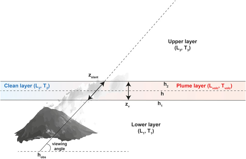
FIGURE 3. Simplified model of the viewing geometry and key parameters defining the measurements. h_obs: observer altitude; viewing angle: zenith angle determining the slant line-of-sight through the atmosphere; h: plume centre height; h₁: plume bottom height; h₂: plume top height; z_v: plume vertical thickness; z_slant: plume thickness along the line-of-sight; L_i: layer radiance; T_i: layer transmittance. In the model, the plume layer contains only the volcanic species, and coexists with the slice of “clean” air in layer 2.

2.2.1 Reference spectra

The first step in the retrieval is to create a set of reference radiance and optical depth spectra for each layer (Figure 4), which are then scaled in the forward model without having to perform computationally expensive radiative transfer calculations. For this task, we use the Reference Forward Model (RFM version 5), a radiative transfer model developed at the University of Oxford (Dudhia, 2017), capable of simulating atmospheric transmittance and emission at high spectral resolution using line data and reference cross-sections for individual gases extracted from the high-resolution transmission molecular absorption database (HITRAN, Rothman et al., 2009). Firstly, we determine the radiance and transmittance of each layer (L_x and T_x) in the absence of a plume. Starting with a standard mid-latitude summer atmospheric profile evaluated with measurements from the Michelson Interferometer for Passive Atmospheric Sounding (MIPAS) (https://eodg.atm.ox.ac.uk/RFM/atm/) and adjusted to reflect present-day CO₂ concentration (400 ppm), we consider a small number of absorbing gases (H₂O, CO₂, N₂O, CH₄ and O₃) over a broad spectral window of 700–1,300 cm⁻¹. The vertical profile is then modified in the layers below 30 km to match the pressure, temperature and relative humidity from a local meteorological balloon sounding taken at a time closest to data acquisition from the station of Trapani in Sicily (launched twice daily and available at https://weather.uwyo.edu/upperair/sounding.html). It should be noted that Trapani is located >100 km west of Stromboli. The sounding might therefore be less representative than desired, and accuracy could be improved with dedicated local soundings. Finally, we resample the profile over an uneven vertical grid (spacing increases with altitude) with 25 layers. The profile is split into the three layers described above (Section 2.2; Figure 3) and RFM simulations are performed to extract radiance (L), transmittance (T), and optical depth (τ) for each of the three layers. Simulations are run with varying amounts of water vapour (21 steps from zero to two times the original concentrations). This allows the forward model to account for changes in relative humidity over the entire profile.

FIGURE 4

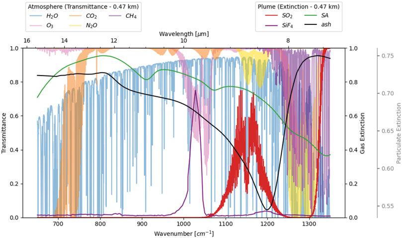
FIGURE 4. Reference spectra for the gases and particles considered in the retrieval. The transmittance of the atmospheric gases in layer two is shown in lighter shades [axis on the left], while the extinction of the plume species is shown in darker shades [axes on the right]. Note that the particulate species are plotted on a separate y-axis [offset to the right in grey] to emphasize their spectral features. Volume mixing ratios for each species were chosen to emphasize spectral shapes and are not necessarily representative of the actual quantities encountered during the retrieval process, except in the case of H₂O, where we show the actual transmittance at plume height. Note the strong water vapour continuum absorption.

Next, we generate reference optical depth spectra for each target volcanic species (SO₂, ash and sulphate aerosols), assuming a homogeneous distribution of gas within layer 2 (Figure 4). Temperature and pressure are derived from the atmospheric profile at the plume height, which was set at around 1 km from visual observations placing the plume just above the craters. The optical depth for each species is derived for any given volume concentration by relating it to the reference concentration as follows:

${\tau }_i=\frac{{\rho }_i}{{\rho }_{i,ref}}{\tau }_{i,ref}(1)$

where τ_i is the optical depth and ρ_i is the volume mixing ratio (VMR in ppmv) for gas i within the layer. Atmospheric gases are also added as “plume” species and allowed to take positive or negative concentrations, which is meant to introduce an ad hoc correction in the forward model to account for small variations of the background gases in each plume measurement.

In addition to absorbing gases, we consider two types of volcanic particles: aqueous sulphate aerosols (SA) and silicate ash. For SA, we consider droplets of a binary solution of H₂SO₄ and H₂O. The H₂SO₄ mixing ratio and relevant temperature can be chosen by the user, and the extinction (${\beta }_{ext}$) and absorption (${\beta }_{abs}$) coefficients are calculated following Mie theory using complex refractive indices found in Lund Myhre et al. (2003) and the PyMieScatt software package (Sumlin et al., 2018). We follow a similar process for ash particles, and the user can choose between refractive indices for natural samples found in previous studies (Reed et al., 2018; Deguine et al., 2020) or calculated based on bulk chemical composition (SiO₂ wt%) using the parameterisation found in Prata et al. (2019). Assuming a reference mass volume concentration of particles (1×10⁻³ g cm⁻³ for ash, 5×10⁻³ g cm⁻³ for SA), the mass is distributed into size bins so that the number fraction follows a log-normal particle size distribution (PSD) around a mean effective diameter (d_eff), which can be set by the user or retrieved as a quantitative parameter. Particle shape is not considered in the model and particles are assumed to be spherical. This assumption is reasonable for SA particles but may lead to significant differences due to inhomogeneous scattering in the case of ash particles. Figure 5 shows the expected variations in shape and intensity of the optical depth spectra in the plume layer for a given mass volume concentration as a function of chemical composition and particle size. As documented previously, the H₂SO₄ mixing ratio has a significant effect on the expected shape of spectral extinction for aqueous SA (Biermann et al., 2000; Sellitto and Legras, 2016). However, we observe rather modest variations when considering a given mass concentration and varying the H₂SO₄ mixing ratios (Figure 5B). Variations in particle size also lead to significant changes in the spectral features of SA (Figure 5A). Consistent with previous observations, we observe an increase in maximum extinction on the order of 20%–30% when the effective diameter increases from .1 μm to 1 μm. For larger particles, the volume to surface area ratio increases dramatically, and the scattering coefficient becomes dominant in the spectral shape, leading to a flattening of the spectral features for a given mass concentration. In this study, we have chosen to fix the chemical composition of the particle species and leave particle size as a free parameter in the retrieval.

FIGURE 5

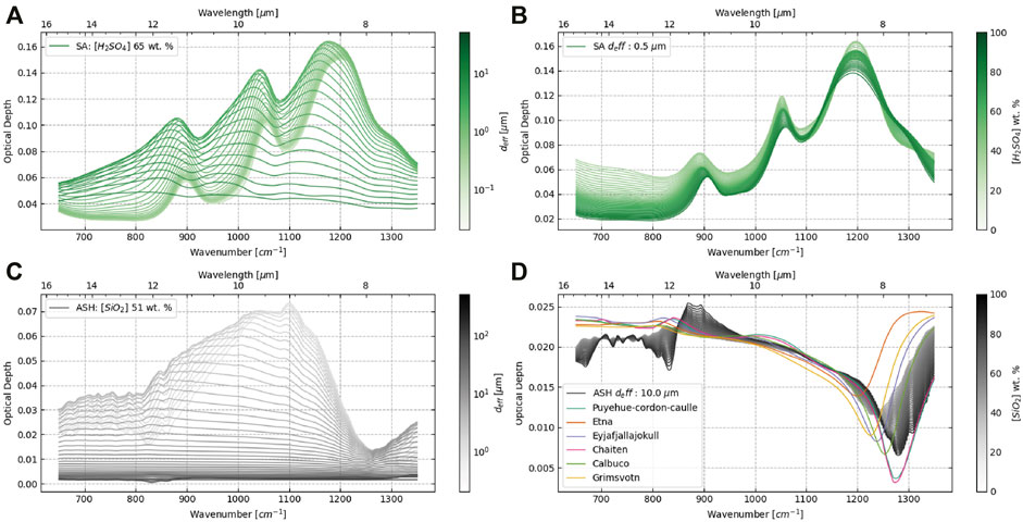
FIGURE 5. Optical depth reference spectra for both particle types considered in the retrieval: sulphate aerosols (SA) ((A,B)—green) and ash ((C, D—grey) (A and C) Optical depth cross sections as a function of particle size. All reference spectra are calculated for the same mass volume concentration of 1x10⁻³ g m⁻³, and only the particle size distribution (PSD) varies. PSDs are log-normal with a mean effective diameter varying according to the colour scale (0.1–10 μm for SA and 0.1–200 μm for ash) and a sigma value of 1.5 (B and D) Optical depth spectra as a function of chemical composition. The effective particle diameter is kept constant (0.5 μm for SA, 10 μm for ash), and only the composition varies. SA compositions range from 38 to 81 wt% H₂SO₄, and spectra are calculated using refractive indices from (Lund Myhre et al., 2003). Ash bulk compositions range from 45 to 80 wt% SiO₂, and spectra are calculated using the parameterization algorithm for complex refractive indices found in (Prata et al., 2019). The mass volume concentration is again fixed at 1x10⁻³ g m⁻³. Also shown are some example spectra calculated for natural samples from recent eruptions with refractive indices found in (Deguine et al., 2020) for the same particle size.

Volcanic ash can be described according to its bulk chemical composition in terms of the relative mass percentage of silica (SiO₂ wt%), with values ranging from 45 wt% for the more basaltic compositions (e.g., Eyjafjallajökull 2010; Sigmundsson et al., 2010) to 75% for the most silicic (e.g., Chaitén 2008; Alfano et al., 2011). In Figures 5A, D a range of attenuations are shown for ash with bulk composition ranging from 45 to 80 wt% SiO₂ using the parameterization developed by Prata et al. (2019), as well as those for a selection of natural samples from several recent eruptions (Reed et al., 2018). For SA, we consider a composition of 65 wt% H₂SO₄ - a value similar to the one recently measured by absorption FTIR spectroscopy for primary aerosols in the Masaya plume (Sellitto et al., 2019)—and use refractive indices measured for this composition by Lund Myhre et al. (2003). Ash optical depth spectra from natural samples follow a general trend with a shift of the spectral minimum and a deepening of the Si-O bond spectral feature as bulk SiO₂ content increases. This dependency of the position and depth of the Si-O bond absorption feature on bulk SiO₂ composition has been thoroughly documented within the planetary science literature (Lyon, 1965; Ramsey and Christensen, 1998; Michalski, 2004; Rogers and Nekvasil, 2015; Henderson et al., 2021), as well as within datasets using natural ash samples from recent eruptions (e.g., Reed et al., 2018; Deguine et al., 2020; Piontek et al., 2021), and is accurately captured by the Prata et al. (2019) parameterization (grey shades in Figure 5D). We use a value of 51 wt% SiO₂ (based on the bulk composition of our sample, see Section 3.1) to calculate the reference extinction spectra for ash. A dependency of the spectral shape on particle size like that observed for SA also exists for ash.

Rather than modelling the measured radiance of a plume spectrum, the forward model replicates the radiance difference at the observer height between a plume measurement and a clear sky measurement (ΔL) from the parameters listed in Table 1. This is done to minimize the effects of the total atmospheric column amounts of background gases and instrument calibration and emphasize the spectral signatures of the volcanic components. The SCDs of all gas and particulate species within the plume layer are retrieved (ash, SA and SO₂), along with ad hoc correction factors for O₃, CO₂, N₂O and CH₄ and a scaling factor for H₂O in all three layers. The size of each particulate species can also be retrieved.

TABLE 1

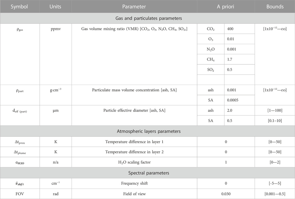
TABLE 1. Retrieved parameters for the forward model along with their bounds and a priori guess.

Following radiative transfer theory, the radiance measured at the observer position (L_obs) in this simplified model can be expressed as:

$L_{obs}=L_1+T_1\left({L_2+T}_2{L}_3\right)(2)$

where L_x represents the radiance and T_x the transmittance of layer x. In the presence of a volcanic plume, the slice of “clean” air in layer 2 (see Figure 3) is replaced by a plume layer, which contains the volcanic components in addition to the atmospheric gases; such that the radiance difference between a plume measurement and a clear sky measurement (ΔL) is:

$\mathit{\Delta }L=T_1\left(L_{plume}-L_2+L_3\left(T_{plume}-T_2\right)\right)(3)$

In the forward model, both the volcanic layer and the clean air slice are assigned separate optical depths. Firstly, we calculate the optical depth of the clean air slice (${\tau }_2$), adjusted for relative changes in water vapour content. The simple linear relationship expressed in Eq. 1) does not hold for H₂O, due to the existence of a continuum absorption, such that an accurate optical depth spectrum cannot simply be scaled from a reference quantity. Instead, we calculate a series of reference spectra for a range of scaling factors (0–2) applied to the original H₂O VMR at plume height. At each wavenumber $\stackrel{\sim }{\upsilon }$, we fit a polynomial to represent the dependency of the optical depth to the adjusted VMR, such that:

${\tau }_{2,\alpha ,\stackrel{\sim }{\upsilon }}={\displaystyle \sum }_{j=0}^p{c}_{j,\stackrel{\sim }{\upsilon }}{\alpha }^j(4)$

where α is the H₂O scaling factor, p is the degree of the polynomial, and c_j is the coefficient in the polynomial expression for the term of degree j. In the forward model, this set of polynomials can be used to accurately calculate optical depth spectra for any continuous value of parameter α as long it is strictly restricted to within the range used in the reference set. This approach avoids having to call RFM to derive H₂O extinction coefficients during the iterative process. We found that this method is computationally much faster than a classical interpolation method and yields accurate results within the bounds of the parameterization. The adjusted transmittance for layer 2 is then simply:

$T_{2,adj}=e^{-{\tau }_{2,adj}}(5)$

Next, we calculate the optical depth of the volcanic species (${\tau }_{volc}$) by summing individual optical depth spectra for each volcanic species:

${\tau }_{volc}={\displaystyle \sum }_i{\tau }_i(6)$

where ${\tau }_i$ is the optical depth for gas i derived from reference spectra calculated at the plume height and temperature using the relationship in Eq. 1). For ash and SA, we use the same polynomial fitting approach expressed in Equation 4 to quantify the relationship between effective particle diameter and optical depth for each wavenumber (see Figure 5):

${\tau }_{i,d_{eff},\stackrel{\sim }{\upsilon }}={\displaystyle \sum }_{j=0}^n{c}_{j,\stackrel{\sim }{\upsilon }}{d_{eff}}^j(7)$

where d_eff is the mean effective diameter of the particles for particulate species i (either ash or SA). This allows the model to accurately calculate optical depth spectra for any continuous value of d_eff within the bounds used in the reference set (0.1–10 μm for SA; 1–200 μm for ash). The transmittance of the volcanic layer (T_volc) is then given simply by:

$T_{volc}=e^{-{\tau }_{volc}}(8)$

The volcanic and clean layers are treated separately (i.e., each given a separate optical depth) but are geometrically occupying the same location. They have identical height, thickness and pressure, but the temperature of the plume species is allowed to differ from that of the ambient gases by a fixed amount (Δt_plume). The radiance for each layer is calculated using the transmittances obtained in equations Eqs. 5, 6, such that the total plume radiance (L_plume) is:

$L_{plume}=B_{t_2}\left(1-T_{2,adj}\right)+B_{\left(t_2+{∆\mathrm{t}}_{plume}\right)}\left(1-T_{plume}\right)(9)$

where B_t is the blackbody radiance calculated using the Planck relationship, t₂ is the atmospheric temperature at plume height, and Δt_plume is the temperature difference between plume and ambient temperature. This temperature difference only affects the radiance of the volcanic components and is usually set to a fixed value in our retrievals. The transmittance of the plume layer (T_plume) is simply the product of the transmittance of both layers:

$T_{plume}=T_{volc}{T}_{2,adj}(10)$

Each atmospheric gas is also included as an individual species in the volcanic layer in order to enable ad hoc corrections to compensate for small differences in total column that could arise between a clear sky measurement and the plume measurement (due to changes in temperature profiles and/or viewing angles). The VMRs and temperature of those gases is fixed within layers 1 and 3 (foreground and background) in the forward model. Adding them as free parameters within the plume layer offers a way of improving the fits around their spectral features. Large variations of the total column of H₂O should also be expected, even over relatively short time windows. These can arise from changes in relative humidity and temperature over the course of the acquisition period. In contrast with previous studies where these large variations are circumvented by using spectral micro-windows in between water vapour absorption lines (e.g., Clarisse et al., 2012; Carboni et al., 2016; Sellitto and Legras, 2016; Sellitto et al., 2019; Guermazi et al., 2021), here we accounted for them using an ad hoc scaling factor for H₂O applied to all layers. Finally, the temperature in the proximal layer (layer 1) can be modified, allowing for small changes in temperature in the proximal layer over the course of a measurement set, which results in a non-uniform offset in the measured radiance difference ΔL. It should be noted that the mathematical expression of the forward model described above does not consider radiance scattered within the line of sight from other directions or multiple scattering.

Up to this point, all computations are performed using high-resolution RFM reference spectra. The last steps in the forward model are to 1) apply a spectral shift to the model grid (the magnitude of the frequency shift is a retrieved parameter); 2) convolve the spectrum with the ILS function (the width of the FOV is also a retrieved parameter, though the retrieved value is stable at 30 mrad throughout all our measurements); and 3) resample the convolved spectrum to match instrument resolution. The resulting radiance difference is the final processed spectrum used in the fitting algorithm. Optimal parameters are determined using an iterative non-linear least-squares method, and the Root Mean Square Error (RMSE) and coefficient of determination (R²) are calculated for the best fit model result.

3 Results

3.1 RPAS ash sample analysis

The ash sample collected during the first measurement campaign in 2019 was analysed for particle size and chemical composition. This section details the results of these analyses, which were used to a) guide the selection of the most appropriate ash refractive indices in the retrieval, and b) compare particle size information between the sample and the values retrieved by the algorithm. The sample’s mass-equivalent PSD (Figure 6) is bimodal, with a population of coarser particles (200–400 μm) and a separate population of finer particles (70–100 μm), seemingly lacking very fine particles. This PSD is generally similar to that of fallout samples collected at the summit of Stromboli in 2015 (Freret-Lorgeril et al., 2019). However, this representation can be misleading, as the Camsizer measurement describes the volume fraction of particles based on their equivalent diameter (X_area: diameter of the area equivalent circle of each particle projection). In these terms, the larger particles take an outsized representation, as the very fine fraction (<10 μm) represents a negligible volume within the overall sample, despite representing the vast majority of the particles. In order to emphasize this effect, we also show the PSD in terms of fractional number density (N-density) of particles by size—calculated based on the measured volume fraction and assuming spherical particles - which is heavily shifted towards smaller particle size bins. The resulting N-density PSD is also bimodal with a large peak around 5–10 μm, and a second one around 65 μm. We argue that the relatively small number of very large particles has a limited effect on the overall optical properties of the ash within the FOV of the OP-FTIR instrument, especially for dilute plumes, and that the comparatively large number of finer particles dictates the shape of the overall extinction profile. Therefore, we believe the N-density PSD is more directly comparable with the sizes retrieved in this work, as the strongest effects on the overall shape of the particle extinction coefficients from Mie scattering largely depend on the number density of particles with diameters close to that of the measured wavelength (i.e., 8–12 μm, see Figure 5).

FIGURE 6

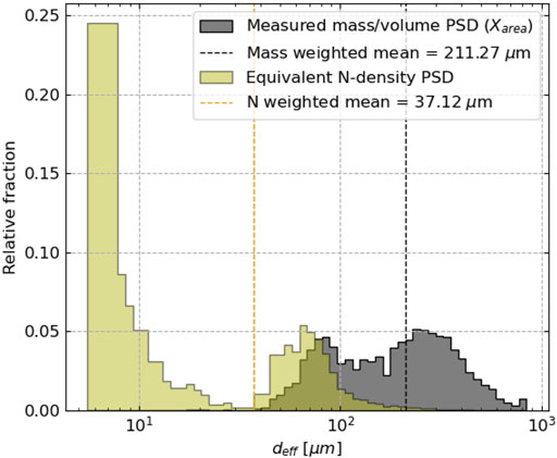
FIGURE 6. Particle size distribution (PSD) measured in the ash sample collected with the RPAS on 11 September 2019. [grey] Original measurement from Camsizer. Volumetric fraction of the particles with regards to their equivalent diameter (X_area: diameter of the area equivalent circle of each particle projection), yielding a mass fraction PSD with a mean at 211.17 μm. [yellow] Number density PSD, where the relative fraction is based on the number of particles instead, converted from volumetric fraction assuming spherical particles. N-density PSD is heavily skewed towards smaller particles (mean of 37.12 μm) and is more directly comparable with retrieved sizes in this work.

The chemical composition of several crystalline phases, as well as the glass matrix as determined via EMPA analysis are presented in Table. 2. The glass composition represents a basaltic trachyandesite, and the main crystalline phases are olivine (Ol), clinopyroxene (Cpx) and plagioclase (Plag). Using the backscattered images from the EPMA analysis, we estimated the relative surface area fractions for each phase (Glass: 60%; Ol: 5%; Cpx: 10%, Plag: 25%) and used these relative fractions to calculate an approximate bulk composition for the sample. This bulk composition (a trachybasalt with ∼51 wt% SiO₂) was used to parameterize the refractive index of the ash during the retrieval (see sect. 2).

TABLE 2

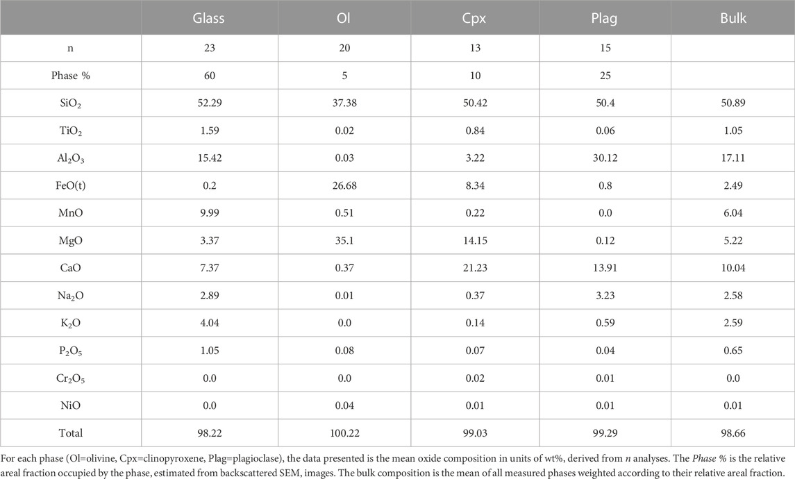
TABLE 2. Chemical composition of crystalline phases and glass measured in the ash sample collected with the RPAS on 11 September 2019.

3.2 Spectral fits

Figure 7 illustrates typical results of individual fits for selected spectra. Over the broad fitting window, the radiance difference spectra are dominated by a broadband contour representing the water vapour continuum. This contour can be positive or negative in absolute value, representing either an increase or a decrease in total water vapour column between the plume and clear sky measurements. The dashed line in the top panel of each figure emphasises this effect and shows the expected difference before considering the contributions from the plume. It is obtained by computing the radiance difference using best-fit parameters for water vapour scaling and observer temperature only and omitting all plume species. The shape of this baseline spectrum at the start of measurements depends on the respective positions of the line-of-sight between clear sky and plume and should approach zero for a clear sky taken at the plume location. Note that this radiance difference already contains recognisable spectral features for H₂O (continuum and narrow absorption/emission lines), O₃ and CO₂ resulting from the overall change in total atmosphere transmission when simply moving the line-of-sight of the instrument. In Figure 7A, showing a spectrum acquired in 2019, O₃ (1,000–1,080 cm⁻¹) and CO₂ (925–1,000 cm⁻¹) appear as emission lines (due to the reduced transmission associated with a H₂O scaling factor <1), and the baseline minimum value goes from −1 to −6 mW/(m²⋅sr⋅cm⁻¹) over the course of ∼30 min. This value is expected to gradually change over the course of measurements, as the background atmospheric conditions evolve. In contrast, Figure 7B shows a spectrum acquired in 2021, where the baseline is a positive radiance difference (H₂O scaling factor >1) and O₃ and CO₂ appear as absorption features. The fitting window was deliberately chosen to include areas on either side where the atmosphere is virtually opaque (<730 cm⁻¹ and >1,270 cm⁻¹). The radiance at those wavelengths represents the blackbody emission at the temperature of the most proximal layer, and we can use the value of the radiance difference to retrieve the temperature of the proximal layer (layer 1).

FIGURE 7

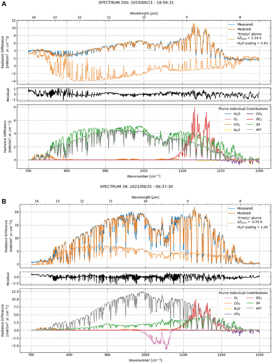
FIGURE 7. Example of fit results for selected individual spectra. In each subpanel: the top plot shows the measured [blue] and modelled [orange] spectra, along with the expected radiance difference without a plume in the line of sight [dotted orange] based on best-fit parameters for water vapour scaling and observer temperature; the middle plot shows the residual between modelled and measured spectra [black]; and the bottom plot shows the individual contribution of each plume species to the modelled spectrum (A) Plume spectrum with both ash and sulphate aerosol (SA) particulates, highlighting the differences in spectral shape between the two species, acquired on 11 September 2019 (B) Ash-rich plume spectrum acquired on 25 September 2021. Note the large O₃ adjustment needed to fit the depth of the measured absorption feature.

The bottom panel in each figure shows the contributions of each plume species (including the ad hoc corrections for atmospheric gases) superimposed over the baseline radiance difference. Each individual contribution is computed using the forward model and zeroing all quantities within the plume except for the species of interest. Note that because the background and foreground atmosphere are always an inherent part of the forward model, water vapour absorption lines still appear in the contribution from each individual species. The most instantly recognisable feature is the emission associated with SO₂. In particulate-rich spectra, a strong O₃ absorption is visible, related to the severe decrease in transmission introduced by the heavy particle burden and often requiring an ad hoc correction.

3.3 Side-by-side IR and UV measurements

Figure 8 shows the time series of SO₂ SCDs retrieved from our FTIR measurements for one dataset acquired during our second measurement campaign in 2021. We also present SO₂ SCDs measured using a co-located UV spectrometer. Disagreement in both absolute values of the SCD and timing of individual peaks are to be expected. They may arise as a consequence of differences in a series of factors between the two methods, such as: 1) the size of the respective FOVs (.03 rad for the IR, .1 rad for the UV); 2) the alignment of the telescopes; 3) the integration time (0.2 s in the UV, 8.9 s in the IR); and 4) different random and systematic error sources between the two methods. The UV time series was smoothed using a kernel of length equal to the IR integration time and resampled to match the temporal x-axis in the IR time series. Moreover, we determined the optimal lag using a cross-correlation method and shifted the UV time series accordingly. We would expect this lag to vary over the course of the measurements, as it is tied to the plume velocity, and plumes associated with crater explosions will travel at greater velocities. However, we found that an overall lag of ∼71 s resulted in a good match between the timing of the main events. Retrieved SCDs between the IR and UV measurements generally agree within a factor of ∼2 (scatter plot in Figure 8A). The main discrepancies occur towards the beginning and end of datasets with the IR method retrieving systematically lower SCDs than the UV method at the beginning of the dataset in Figure 8A, and systematically higher SCDs towards the end of the dataset.

FIGURE 8

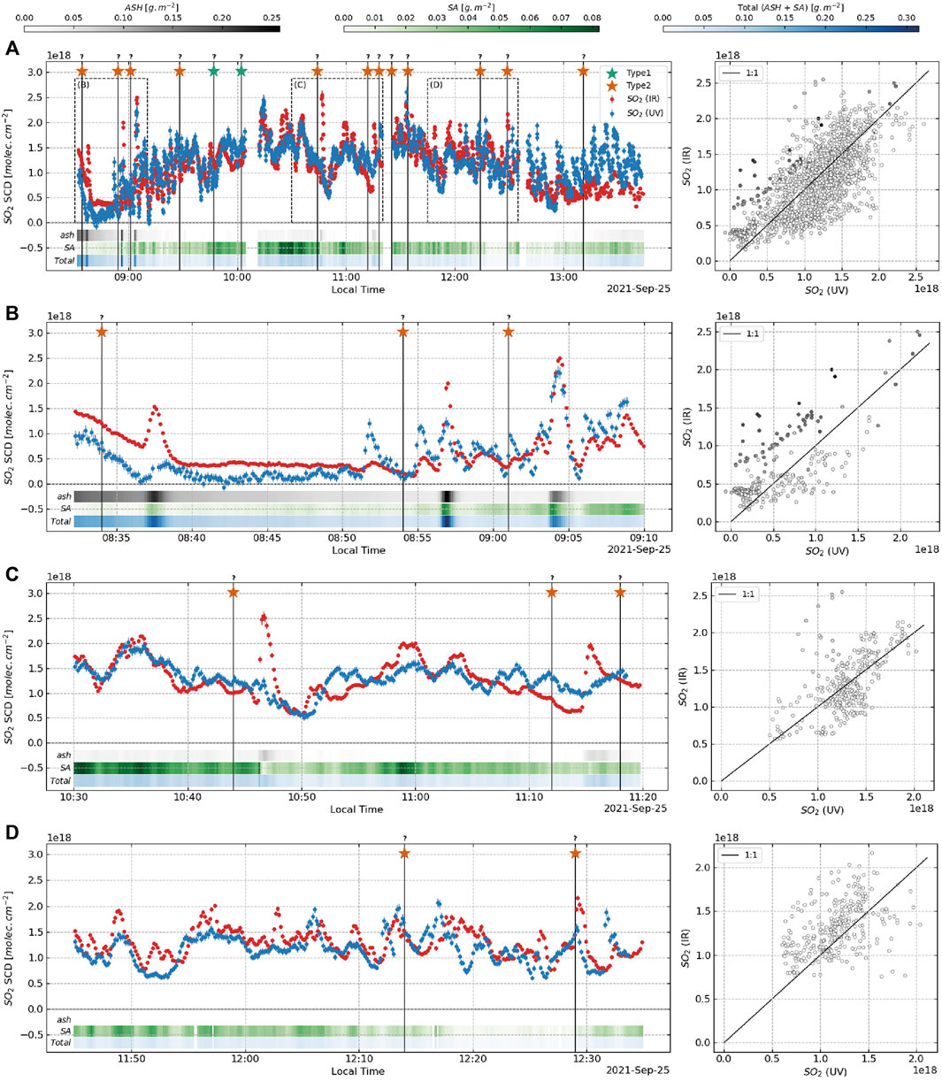
FIGURE 8. Time series of SO₂ SCDs measured on 25 September 2021. SCDs retrieved from the IR dataset are shown in red. SCDs retrieved from UV measurements are shown in blue. The UV time series was resampled after cross-correlation and has been shifted by 71 s to correct for the misalignment between the telescopes. Also shown are the mass SCDs for ash [grey], sulphate aerosols [SA, green] and total particulates [blue]. Stars represent individual events, recorded at the time when a plume is visible over the crater rim in video footage. Inset on the right shows a scatter plot between UV and IR SCDs, and the datapoints are coloured according to the retrieved ash SCD. Time and y-axis scales change between panels, but colour scales remain the same (A) Full dataset. Zoom windows for subsequent panels are shown as dashed boxes. Note that systematic disagreement between UV and IR retrieval occur towards the beginning and end of the measurement periods (B) Zoom window showing three ash-bearing events between 08:30 and 09:10. Most data points departing from the 1:1 line on the scatter plot are associated with higher ash burdens. Note the relatively high ash burden during the first 7–8 min leading to the first ash event and the corresponding disagreement between UV and IR retrievals during that period (C) Zoom window showing two ash-bearing events between 10:30 and 11:20. Note that relatively high SA SCDs before the first event do not lead to significant disagreement between UV and IR retrievals (D) Zoom window with no ash-bearing event between 11:45 and 12:35. Note the change in scale in the ash SCD colour scale.

Figure 8 further documents explosive events, as recorded in GoPro time-lapse footage (orange stars). Here we only report ash explosions, defined as type 1 events following the terminology in Patrick et al. (2007), and mark them at the time of their first appearance above the crater rim from our vantage point. Type 2 events (essentially bubble bursts associated with ballistics) were much more difficult to identify from the 2021 vantage point without a direct view of the craters (Figure 1). It is also impossible to assign a specific crater of origin for individual events for the 2021 time series. All documented events are followed by a marked increase in retrieved SO₂, SA and ash contents, after a delay of 1-2 min representing the time needed for the plume to move into the FOV of the instruments.

3.4 Near-vent measurements

During the 2019 campaign, we performed measurements from the l’Osservatorio restaurant, with a direct view of the crater area (Figure 1B). We were able to move the FOV of the instrument to intersect the plume directly above the vent. A time series of the retrieved quantities for a dataset collected in this configuration is shown in Figure 9. During this period, we captured the baseline passive degassing plume, as well as plumes resulting from explosive events. Events were documented through visual observation and logged manually. As we had a direct view of the crater area, the explosive plumes can be separated into two classes with relation to the event types defined by Patrick et al. (2007). Type 1 events (bubble bursts + ballistics) produce plumes with low ash content and elevated concentrations of SO₂ (green stars). Type 2 events, on the other hand, are ash-rich with a visibly dark plume (orange stars). The FOV of the instrument was positioned directly above the NE crater area. As a result, this dataset mainly contains events originating from the NE and central vents (which were directly behind the NE vents along the line of sight). Some emissions from the SW crater area may have entered our FOV but, given the wind direction during our measurements, this was challenging to determine visually. Type 1 events originated from both NE and C areas, and type 2 events mainly originated from the NE craters. Absolute retrieved SCDs for SO₂, ash and sulphate aerosols above the vents are relatively high (peak SO₂: 6 × 10¹⁸ molec⋅cm⁻², peak ash: 1.75 g⋅m⁻², peak SA: 1.2 g⋅m⁻²). Peaks in SO₂ within the time series generally occur shortly after the onset of each event. Retrieved SA particle sizes are shown in the bottom plot in Figures 9E, F. The probability density function, where each measurement of particle size is weighed according to the associated SCD, exhibits a mode around .8 μm, representative of the typical size retrieved during low level degassing (mean d_eff value of 1.79 ± 3.08 μm). There are also several peaks at higher diameters, representing d_eff values retrieved during the explosive events (i.e., type 2 ca 18:56, 18:58 and 19:02 and type 1 ca 18:36 and 18:43, Figure 9E).

FIGURE 9

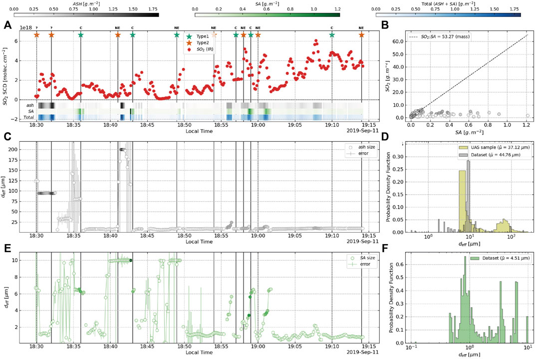
FIGURE 9. Time series of retrieved quantities for a dataset collected directly above the vents on 11 September 2019 (A) SO₂ SCDs [red]. Error bars represent the modelling error only (i.e., the covariance estimated during the linear regression). Stars represent individual events visually documented in the crater area (type 1 or 2), labelled according to the vent from which they originated (NE: northeast; C central). The mass SCDs for ash [grey], sulphate aerosols [SA, green], and the total particulates [blue] for each individual measurement are also shown in colour bars located at the bottom of the plot (colour scales at the top) (B) Scatter plot between SO₂ and SA SCDs, and the linear fit for this data (SO₂/SA ratio = 53.27). Individual data points are coloured according to the ash SCD (C) Retrieved effective diameter for ash particles (D) Histogram of the retrieved ash sizes over the entire dataset [light grey] weighted according to the ash SCD to minimise the importance of measurements with very low amounts of ash. For comparison the particle size distribution measured in the ash sample collected with the RPAS is also shown [yellow] (E) Retrieved effective diameters for the SA (F) Histogram of the retrieved sizes over the entire dataset [light green] weighted according to the SA SCD to minimise the importance of measurements with very low amounts of SA. Note that size distributions for both ash and SA are bimodal.

In a scatter plot between SO₂ and SA over the entire dataset (Figure 9B), the measurements with lower amounts of particulates (light shades) define a ratio line. We calculate SO₂/SA mass ratios using a robust linear regression (Siegel, 1982) which emphasises the overall trend rather than more extreme data points, in order to minimise the effects of those measurements with high amounts of particulates during the explosive events. This is done so we can quantify the sulphur partitioning in the gas plume during passive degassing periods. We observe a ratio of ∼53 by mass in this dataset. Values from similar datasets range between 40 and 80.

Retrieved ash particle sizes are shown in the middle plot in Figures 9C, D. The retrieved size for ash particles increases during explosive events. The probability density function exhibits a clear mode at ∼10 μm during non-explosive phases (range between 5 and 15 μm). During the most intense ash-rich type 2 events (e.g., ca 18:30–18:33 and ca 18:42 in Figure 10), ash d_eff reaches much higher values, up to 200 μm, the upper bound for ash size set in the algorithm. During type 2 events of lower intensity (e.g., three events in quick succession ca. 18:56, 18:58 and 19:00), particle size also increases during each event, but to lower values of 10–30 μm.

FIGURE 10

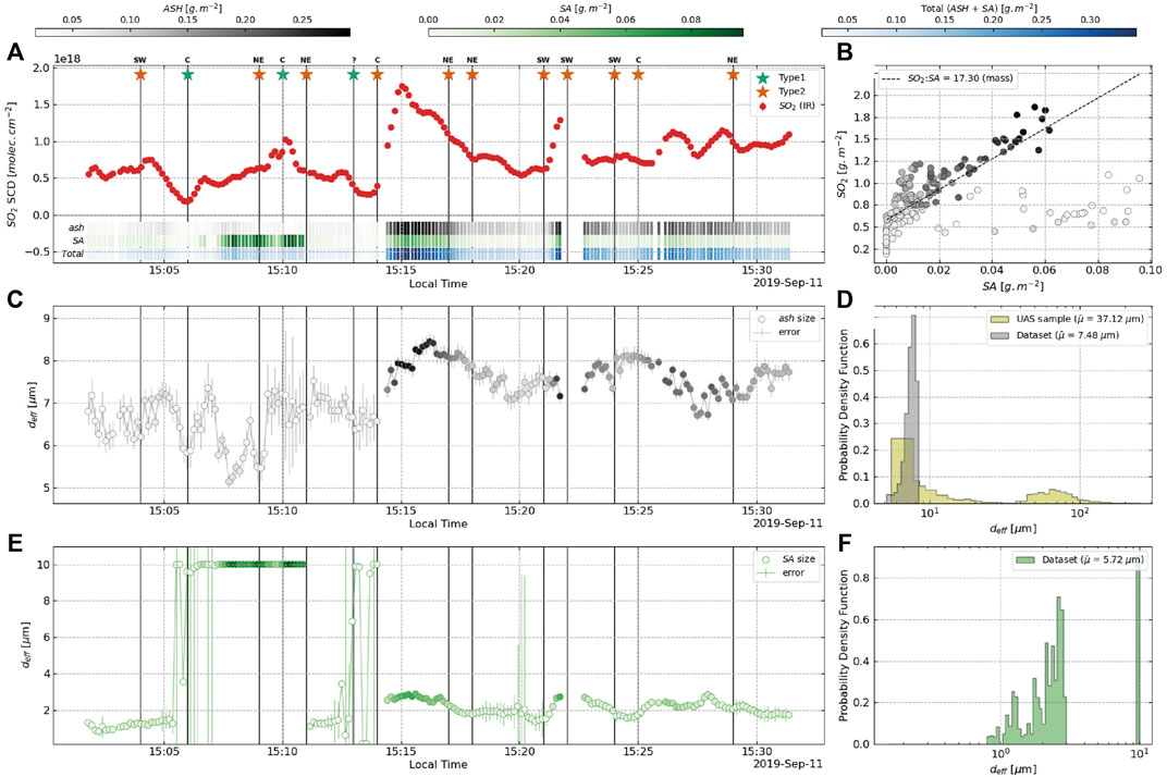
FIGURE 10. Time series of retrieved quantities for a dataset collected downwind on 11 September 2019 (A) SO₂ SCDs [red]. Error bars represent the modelling error only (i.e., the covariance estimated during the linear regression). Stars represent individual events visually documented in the crater area (type 1 or 2), labelled according to the vent from which they originated (NE: northeast; C central; SW: southwest; ? unknown). The mass SCDs for ash [grey], sulphate aerosols [SA, green], and the total particulates [blue] for each individual measurement are also shown in colour bars located at the bottom of the plot (colour scales at the top) (B) Scatter plot between SO₂ and SA SCDs, and the linear fit for this data (SO₂/SA ratio = 17.3). Individual data points are coloured according to the ash SCD (C) Retrieved effective diameter for ash particle (D) Histogram (N density) of the retrieved sizes over the entire dataset [light grey] weighted according to the ash SCD so that sizes retrieved during ash bursts are represented more heavily. For comparison the particle size distribution measured in the sample collected with the RPAS is also shown [yellow] (E) Retrieved effective diameters for the SA (F) Histogram of the retrieved sizes over the entire dataset [light green] weighted according to the SA SCD.

3.5 Downwind measurements

Figure 10 shows a time series of measurements acquired from the same vantage point and on the same day (11 September 2019) as those measurements shown in Figure 9, but where the instrument FOV intersected the plume ∼0.8 km downwind (Figure 1B). The measured SCDs for all target species (peak SO₂: 2 × 10¹⁸ molec⋅cm⁻², peak ash: .3 g⋅m⁻², peak SA: .1 g⋅m⁻²) are lower than in the near-vent measurements, representing the dilution of the plume and loss processes (e.g., SO₂ oxidation and settling of PM) as it travels. Wind speed on that day was relatively low, and this distance corresponds to a plume age of approximately 3–5 min. Recorded type 1 and type 2 events at the vents appear disassociated with peaks in the SO₂ time series. However, we identify three individual events within the time series: one event with elevated SO₂ and SA, with a slow onset at ca. 15:07, assumed to be a type 2 event), and two events with sharper onsets at ca. 15:14 and 15:21 showing elevated SO₂, SA and ash contents (assumed to be type 2 events). The mean SO₂/SA mass ratio for this particular dataset is ∼17, and values for downwind datasets range between 10 and 30.

Retrieved sizes for the SA downwind are 5.21 ± 4.27 μm during low level degassing, and 2.19 ± 0.36 μm on average during explosive events (type 1 and type 2). Sizes retrieved during a type 1 event with a high SA SCD (ca 15:07–15:10 in Figure 10) show elevated values, reaching the upper bound for SA size set in the algorithm (10 μm). Retrieved sizes for ash in the downwind dataset are 6.66 ± 0.57 μm outside of ash-rich events, and 7.68 ± 0.38 during ash-rich events. Both values are in good agreement with the smaller mode of the particle size distribution found in our collected sample (Figure 6).

4 Discussion

4.1 Sensitivity to plume temperature

The principal source of uncertainty in the method comes from the estimation of plume temperature in the FTIR forward model. This is illustrated by systematic disagreements between the UV and IR retrievals of SO₂ SCDs towards the beginning and end of datasets (see Figure 8A). As the measurement period evolves, the actual temperature at plume height increases or decreases (depending on time of day), while the assumed plume temperature in our model remains the same (extracted from the reference atmospheric sounding, which is taken only in 12 h intervals, and at a location >100 km away from the measurement location). If the assumed temperature is colder than the plume actually is, the amount of SO₂ retrieved by our method will be an overestimate of the actual SO₂ in the plume. Conversely, if the assumed temperature is warmer than the actual temperature, our measurements will be an underestimate. UV spectroscopy is not affected by this assumption and thus differences may arise between the retrieved quantities from the FTIR and the UV measurements. A further complication is that both plume height and atmospheric temperature at plume height may vary over the course of the measurements, leading to systematic errors in all quantities retrieved by the method. As the radiance difference is calculated using a clear sky spectrum acquired at the beginning or end of the measurements, exacerbating the differences in measured radiance which result from changing atmospheric conditions in spectra collected further away from the calibration period, using more frequent clear sky measurements will yield more consistent results. In addition, plume temperature might be higher due to the presence of the volcanic plume, i.e., the actual temperature in layer 2 may differ from the one recorded in the atmospheric profile due to the hot volcanic gas and particles.

To quantify the error linked with the plume layer temperature, we introduced a fixed temperature difference (Δt_plume) between the temperature in the volcanic layer at the time of measurement and the clean air layer temperature in the clear sky measurement and performed the retrieval on a subset of 1,000 measurements from 25 September 2021, for various values of Δt_plume (Figure 11). The temperature of the plume at Stromboli is frequently recorded using a Multi-component Gas Analyser System (Multi-GAS) at the summit (Aiuppa et al., 2009; Aiuppa et al., 2010). Although temperature measurements are not reported in published studies, they are recorded by the instrument and typically fall within 1–3 degrees of the ambient temperature when the plume drifts over the summit (INGV personal communication). Therefore, we vary Δt_plume between values of −5 K and + 5 K. In addition, we ran the retrieval on the same data subset leaving the temperature of the volcanic layer as a free parameter. This latter approach yielded unrealistic results, with Δt_plume ranging from −30 K to + 30 K within the same dataset, leading to overestimates of up to a factor of four in the retrieved SO₂ SCD in spectra with the highest amounts of particulates. However, these results allow us to quantify the expected errors related to plume temperature. When plotting the ratio between the SO₂ SCD retrieved with a free t_plume and the SO₂ SCD retrieved with a fixed t_plume against the associated Δt_plume, they outline a very clear relationship, which can be approximated using an exponential decay function. We estimate that uncertainties in assumed plume temperature will lead to errors in the retrieved SO₂ SCDs of a factor of ∼3.5% per K. When considering a realistic range of assumed plume temperatures, this translates to overestimates of up to 19% (Δt_plume = −5 K) and underestimates of up 16% (Δt_plume = + 5 K). Measurements with high SCDs of particulates depart from this overall relationship and introduce larger overestimates. Similar values are found when examining other retrieved quantities (summarised in Table 3). These uncertainties are much larger than the typical fitting error of ∼2.2% and represent the largest limitation in the method. Local measurements of temperature at plume height and accurate visual determination of the plume height will help mitigate the potential for error.

FIGURE 11

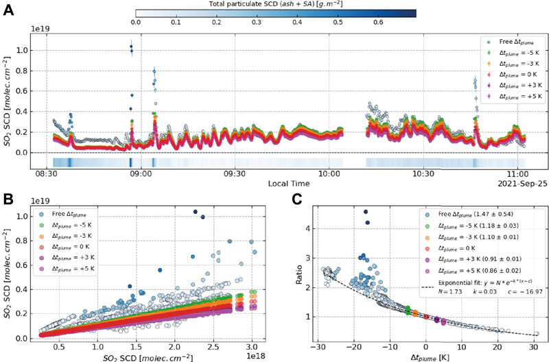
FIGURE 11. Sensitivity analysis of the effect of plume temperature on the retrieved SO₂ SCDs. (A) Time series of SO₂ SCDs for a subset of 1,000 spectra measured on 25 September 2021, using various values of Δt_plume (green: −5 K; orange: −3 K; red: 0 K; purple: +3 K; magenta: +5 K; blue: free parameter). Bar plot at the bottom shows the total SCD for all particulate species (colour scale at the top), highlighting the eruptive events with high ash or sulphate aerosols (SA). Data points in the free T_plume retrieval are also coloured according to the total particulate SCD (B) Retrieved SO₂ SCDs for each of the time series mentioned above against the corresponding SO₂ SCD in the reference retrieval (Δt_plume = 0 K). Note that measurements with high amounts of particulates produce larger overestimates in the retrieved SO₂ (C) Ratio between retrieved SO₂ in each time series against the reference retrieval (Δt_plume = 0 K). Measurements with low particulate content outline an exponential relationship, with an expected uncertainty of ∼3.5% per K.

TABLE 3

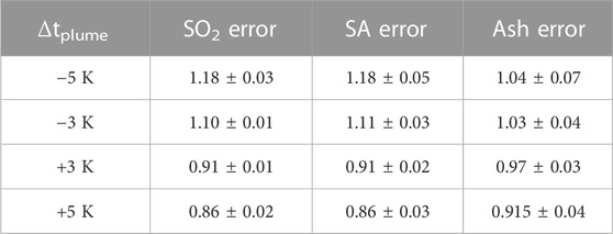
TABLE 3. Estimated errors associated with plume temperature. Expressed as the ratio of the retrieved SCD over a reference dataset with Δt_plume = 0 K.

4.2 Plumes with high optical thickness

Previous measurements have shown the PM-related optical properties of the Stromboli plume to vary with the occurrence of individual events (Sellitto et al., 2021). Our results further support these observations, with type 1 events generally associated with a peak in SO₂ SCD, and an increase in SA SCD, whereas type 2 events are associated with increased amounts of both ash and SA SCD (Figure 9). Some type 1 and type 2 events were not accompanied by particle increases and in one case no SO₂ peak was observed. This may reflect the fact that some plumes drifted above the FOV of our instrument, either because the explosion that produced them injected significant momentum into the plumes, or because shifts in wind direction or speed caused the plume to rise more vertically in some cases than others. As the dataset shown in Figure 9 was acquired in the run up to sunset (approximately 19:15 local time), it is also possible that our manual observations are incomplete or inaccurate, particularly towards the end of the dataset as it became darker.

The presence of high amounts of particulates within a plume (e.g., ash-bearing plumes after explosions or those with a high optical thickness due to large amounts of aerosols) can negatively affect UV measurements and lead to large errors in retrieved SO₂ SCDs if realistic radiative transfer is not taken into account (Kern et al., 2010; Kern et al., 2012; Kern et al., 2013; Varnam et al., 2020). Although both over- and underestimations are possible, depending on the specific conditions within a plume (i.e., magnitude of the SO₂ column amounts and nature of the scattering aerosol), underestimates are more likely in plumes with high optical thicknesses, particularly if the particulate species within the plume also exhibit strong absorbing properties, as is the case for ash-laden plumes captured close to the vent (Kern et al., 2013). In such cases, IR retrievals may offer an advantage, as they are less likely to be impacted by multiple scatterings (typical sizes for volcanic particles are often much smaller than the 8–12 μm wavelength range of the method) and by light dilution effects. Our method offers a means of quantifying the aerosol optical thickness and SO₂ SCDs from a single measurement. For optically thick plumes containing very large amounts of ash or PM, underestimates in our IR retrievals should still be expected, as the radiance collected at the instrument would originate mainly from the surface of the plume. However, for moderate particle concentrations, our method offers a way to compensate for the expected loss of radiance from within the plume layer. This is apparent at several points in the time series presented in Figure 8 and highlighted in subpanels B-C, where ash-rich plumes are generally associated with higher retrieved SO₂ SCDs in the IR, by factors ranging from 2 to 5. We propose that this represents an underestimate of the true SO₂ burden by the UV method, and that the SCDs retrieved in the IR are closer to the concentrations within the plume at the time of measurement. Alternatively, it is possible that plumes with high amounts of ash retain heat more efficiently, and as a result the assumption of a plume in thermal equilibrium with the atmosphere is no longer valid. In such a case, the retrieved SO₂ SCD with the IR method would constitute an overestimate of the real values, as warmer plumes emit more radiation. These discrepancies merit further investigation within a dedicated, systematic side-by-side experiment in which multiple scattering and light dilution effects are accounted for in both UV and IR retrievals.

4.3 Sulphur speciation during plume transport

Table 4 summarises sulphur speciation values previously reported and measured in proximal plumes (<1 km from source) at Stromboli and elsewhere. Sulphur partitioning between the gas and aerosol phases is generally reported as the molar ratio of SO₄^2- ions to SO₂ (SO₄^2-/SO₂) when measured with filter packs. Alternatively, when retrieved with spectroscopic techniques, the reported value is often the mass ratio of the gas phase over the aerosol phase, including the water (SO₂/SA). The conversion between the two values depends on the acidity of the aerosols themselves, which is not always reported. For a simple comparison, we assume an acidity of 65 wt% H₂SO₄ (the value used to generate our reference extinction spectra), and present both ratios. The SO₂/SA measured in our near-vent measurements is on the lower side of the range observed in proximal plumes at other volcanoes, suggesting the presence of large amounts of primary sulphate aerosols (i.e., those condensed directly from the high-temperature gas emitted from the magma) in the passive plume and during type 1 events (which typically have lower particulate loads than type 2 events). Alternatively, this could reflect the rapid formation of sulphate via oxidation of SO₂ condensing onto the primary particles in the plume or a higher water content of the SA in our measurements. This is supported by the observations that the sizes measured here (Figure 9) are rather large compared to those expected for newly formed particles (<.1 μm for particles within the “nucleation mode”) (Whitby, 1978; Mather et al., 2003b).

TABLE 4

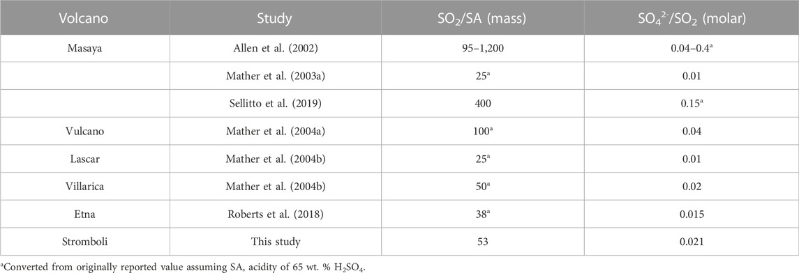
TABLE 4. Sulphur speciation in proximal volcanic plumes from this and previous studies.

SO₂/SA ratios in diluted downwind datasets (range 10–30, mean of ∼17 in the dataset illustrated in Figure 10) are lower than those found near-vent (range 40–80, mean of ∼53 in the dataset illustrated in Figure 9), suggesting either an increase in sulphate aerosol mass and/or a decrease in SO₂ mass as the plume ages. Several mechanisms exist which could explain the observed decrease in SO₂/SA ratio with plume age. SO₂ depletion by oxidation into sulphuric acid is a commonly proposed mechanism (Eatough et al., 1994) and has been documented in volcanic plumes, with SO₂ loss rates in tropospheric plumes ranging between 10⁻⁷ and 10⁻³ s⁻¹ (Oppenheimer et al., 1998b; McGonigle et al., 2004; Rodríguez et al., 2008). As SO₂ is oxidized, the decrease in SO₂/SA ratio then results from both a loss of gaseous SO₂ in the plume, and from condensation of sulphate formed as SO₂ is oxidized, either increasing the size of existing particles, or nucleating new particles, and ultimately causing an increase in aerosol mass. However, even assuming a fast depletion rate at the upper bound of the range documented above (10⁻³ s⁻¹), it is not clear that this oxidation process would be fast enough to explain the changes observed here, which took place over distances of <1 km and for plume ages of only a few minutes. Alternatively, the mass of SA may also be increased by condensation of water into the aerosol, a process by which the existing sulphate aerosols lower the supersaturation threshold required to grow droplets (Mather et al., 2004a; Mather et al., 2004b), potentially ultimately acting as seeds for the formation of clouds (Pianezze et al., 2019). This process would increase the overall mass of the SA while decreasing their relative acidity. Given the fixed parameter for SA acidity in our retrieval, our model is not able to measure this change in acidity. However, hygroscopic growth is consistent with both the slight increase in retrieved SA size (during periods of passive degassing) and the decrease in SO₂/SA mass ratio in the downwind measurements and is therefore a plausible mechanism to explain our observations. Two recent studies have investigated the evolution of SO₂ and SA in the Stromboli and Etna plume (Pianezze et al., 2019; Sahyoun et al., 2019). Both studies found an increase in the number concentration of SA particles with distance from the vent, combined with an increase in the size of the measured particles. Although the mechanisms investigated by these studies take place over much larger distances and targeting older plumes, their interpretations are broadly consistent with our observations, and suggest the mechanisms of particle growth that ultimately can result in cloud condensation occur even in very young plumes such as those we measured. Further investigation of these mechanisms might elucidate volcanic impacts and interactions with cloud cover in the troposphere (e.g., Ebmeier et al., 2014).

4.4 Ash settling during plume transport

As mentioned previously, the sensitivity of the retrieval to particle sizes above 20 μm is not well established, and it is possible that the retrieved values do not represent the true size within the plume. Nevertheless, our observations of significant increases in optical depth in the long-wave infrared spectrum and rapid shifts in particle size during type 2 events are consistent with the increase in aerosol optical depth and decrease in the Angstrom exponent observed at shorter wavelengths by Sellitto et al. (2021) and are the likely the result of an injection of coarser particles from the explosions. Sizes retrieved over the entirety of the dataset capture the full range of ash particle sizes found in the sample collected with the RPAS, with the fine fraction often found during low-level degassing and the coarser particles during type 2 events.

The size of ash retrieved in diluted plumes (either downwind or above the vent during non-explosive activity) is remarkably consistent, with values of 5–10 μm in both datasets. This value is also consistent with the fine size fraction in our collected sample. Coarser particles (65–200 μm) retrieved from near-vent measurements are not detected in the downwind measurements, even when a high SCD of ash is retrieved, suggesting that they have already been removed by sedimentation at that point. This is consistent with our visual observations during the measurement period of large “fingers” of ash raining from the drifting plumes and depositing the coarser particles on the slopes of the volcano, as documented in Freret-Lorgeril et al. (2020). It is also consistent with the observations of Sellitto et al. (2020) who found a decrease in aerosol size with increasing distance from the vent in the proximal (<20 km) plume at Etna volcano, which they interpreted as due to the sedimentation of ash (and possibly coarser SA). It should be noted that the sensitivity of the IR retrieval to particle size is most pronounced in the range of particle sizes 1–10 μm, where the size of the particles approaches the wavelength of radiation. The spectral shape for ash shows relatively little variation with increasing sizes above 20 μm (see Figure 5), and the detection of coarser particle sizes in this work should be taken as an indication of their presence rather than an accurate determination of their actual size.

5 Conclusion and future work

Here we present a new method for simultaneous quantification of gases and particulates in volcanic plumes using emission OP-FTIR measurements. Using a broad fitting window, the method allows for identification and quantification of ash and sulphate aerosols within a plume, and the determination of particle size. Retrieved SO₂ column densities are in reasonable agreement (within a factor of 2) with those retrieved using UV spectroscopy with the larger discrepancies occurring during ash-rich events. SO₂ SCDs retrieved with the IR method are generally larger than those retrieved with traditional UV methods. The ability to measure particles and gas simultaneously could prove useful in understanding and quantifying the underestimation of SO₂ column densities by UV methods which results from multiple scattering, either in plumes containing large amounts of particulates or when measurements are performed from large distances (e.g., Kern et al., 2013; Campion et al., 2014; Varnam et al., 2020). This invites further investigation of ash- and SA-rich plumes using simultaneous measurements with both methods.

Using this new methodology, we document the plume composition during different types of volcanic activity at Stromboli (passive degassing, type 1 ash-poor and type 2 ash-rich explosions) and its evolution over a short distance downwind of the active vent. Our algorithm consistently identifies a fine ash fraction (5–10 μm) present even during non-explosive phases and in distal plumes, as well as coarser ash particles (30–200 μm, ∼65 μm mean) found only in datasets collected near the vent after type 2 events. We collected an in-situ sample of ash during an explosive event using a Remotely Piloted Aircraft System (RPAS), allowing us to compare particle sizes measured remotely with those found directly within the plume. Both size modes detected by our FTIR method were found in the RPAS sample, providing validation for the retrieval algorithm. The measured loss of the coarse ash size at a short distance (∼.8 km) from the vent is consistent with visual observations of particle settling below the drifting plume. Measurements of SA size (slightly coarser particles found in downwind datasets) and SO₂/SA mass ratios (from 53 near the vent to 17 downwind) suggest rapid aerosol growth over these short distances as well, which we propose to be dominated by water uptake. Long-term deployment of this method might provide useful additional metrics alongside a baseline of SO₂ data to investigate physical and chemical processes occurring within tropospheric plumes over short (1–10 km) distances. Emission IR measurements also enable measurements during periods when UV methods cannot be used (i.e., at night) and without the need to align the spectrometer with an IR source, opening the possibility for flexible 24 h gas monitoring.

Given the encouraging results reported here, we suggest the method should be further developed to explore its full potential. Future work will focus on longer term deployment at Stromboli and other volcanoes, with the aim of creating time series spanning days or weeks, and to evaluate the usefulness of the method for continuous monitoring. As well, systematic comparison with UV retrievals should be explored, with the aim of improving SO₂ quantification in particulate-rich plumes. Finally, a number of improvements and extensions should be tested and implemented within the source code: 1) fitting of individual absorption lines for gases such as CO₂ following the method outlined in Goff et al. (2001); 2) quantitative retrieval of SiF₄; 3) improved spectral fits focused on the particulate species using spectral micro-windows in order to alleviate the effects of water vapour absorption; and 4) exploring the evolution in aerosol composition by fixing the particle size and targeting SA particle composition, including the possibility of sulphate-coated ash particles.

Data availability statement

The raw data supporting the conclusions of this article will be made available by the authors, without undue reservation.

Author contributions

J-FS designed and supervised the measurement campaigns, developed the algorithm, processed the data and wrote the manuscript first draft. TM and MB supervised all work, participated in field campaigns and assisted in the development of the algorithm. AS provided the OP-FTIR instrument, assisted in data collection and analysis. BE and MV assisted in the collection and analysis of UV measurements, RG advised on the implementation of the quantitative retrieval for particulates. All authors edited the manuscript.

Funding

The work outlined in this manuscript was supported by NERC award NE/S004025/1.

Acknowledgments

The authors would like to thank INGV-Catania, and particularly Giuseppe Salerno, for facilitating access to Stromboli volcano during the field campaigns and for loaning UV equipment. We would also like to thank Evgenia Ilyinskaya for her help in the PSD analysis of the ash sample, Zoltán Taracsák for performing the EMPA measurements, and Anu Dudhia for insightful discussions about the physics behind the method and the use of the RFM software. We also thank Simon Carn, Pasquale Sellitto and Wolfgang Stremme for their insightful comments and suggestions which led to significant improvement of the manuscript. For the purpose of Open Access, the author has applied a CC BY public copyright licence to any Author Accepted Manuscript (AAM) version arising from this submission.

Conflict of interest

The authors declare that the research was conducted in the absence of any commercial or financial relationships that could be construed as a potential conflict of interest.

Publisher’s note

All claims expressed in this article are solely those of the authors and do not necessarily represent those of their affiliated organizations, or those of the publisher, the editors and the reviewers. Any product that may be evaluated in this article, or claim that may be made by its manufacturer, is not guaranteed or endorsed by the publisher.

References

Aiuppa, A., Federico, C., Giudice, G., Giuffrida, G., Guida, R., Gurrieri, S., et al. (2009). The 2007 eruption of Stromboli volcano: Insights from real-time measurement of the volcanic gas plume CO₂/SO₂ ratio. J. Volcanol. Geotherm. Res. 182, 221–230. doi:10.1016/j.jvolgeores.2008.09.013

CrossRef Full Text | Google Scholar

Aiuppa, A., Bertagnini, A., Métrich, N., Moretti, R., Di Muro, A., Liuzzo, M., et al. (2010). A model of degassing for Stromboli volcano. Earth Planet. Sci. Lett. 295, 195–204. doi:10.1016/j.epsl.2010.03.040

CrossRef Full Text | Google Scholar

Alfano, F., Bonadonna, C., Volentik, A. C. M., Connor, C. B., Watt, S. F. L., Pyle, D. M., et al. (2011). Tephra stratigraphy and eruptive volume of the May, 2008, Chaitén eruption, Chile. Bull. Volcanol. 73, 613–630. doi:10.1007/s00445-010-0428-x

CrossRef Full Text | Google Scholar

Allard, P., Burton, M., and Muré, F. (2005). Spectroscopic evidence for a lava fountain driven by previously accumulated magmatic gas. Nature 433, 407–410. doi:10.1038/nature03246

PubMed Abstract | CrossRef Full Text | Google Scholar

Allard, P., Burton, M., Sawyer, G., and Bani, P. (2016). Degassing dynamics of basaltic lava lake at a top-ranking volatile emitter: Ambrym volcano, Vanuatu arc. Earth Planet. Sci. Lett. 448, 69–80. doi:10.1016/j.epsl.2016.05.014

CrossRef Full Text | Google Scholar

Allen, A. G., Oppenheimer, C., Ferm, M., Baxter, P. J., Horrocks, L. A., Galle, B., et al. (2002). Primary sulfate aerosol and associated emissions from Masaya volcano, Nicaragua: Primary sulfate aerosol from masaya volcano. J.-Geophys.-Res. 107, ACH 5-1–ACH 5-8. doi:10.1029/2002JD002120

CrossRef Full Text | Google Scholar

Barsotti, S., Andronico, D., Neri, A., Del Carlo, P., Baxter, P. J., Aspinall, W. P., et al. (2010). Quantitative assessment of volcanic ash hazards for health and infrastructure at Mt. Etna (Italy) by numerical simulation. J. Volcanol. Geotherm. Res. 192, 85–96. doi:10.1016/j.jvolgeores.2010.02.011

CrossRef Full Text | Google Scholar

Biermann, U. M., Luo, B. P., and Peter, Th. (2000). Absorption spectra and optical constants of binary and ternary solutions of H₂SO₄, HNO₃, and H₂O in the mid infrared at atmospheric temperatures. J. Phys. Chem. A 104, 783–793. doi:10.1021/jp992349i

CrossRef Full Text | Google Scholar

Burton, M. R., Oppenheimer, O., Horrocks, L. A., and Francis, P. W. (2000). Remote sensing of CO₂ and H₂O emission rates from Masaya volcano, Nicaragua. Geology 28, 915–918. doi:10.1130/0091-7613(2000)028<0915:rsocah>2.3.co;2

CrossRef Full Text | Google Scholar

Burton, M. R., Oppenheimer, C., Horrocks, L. A., and Francis, P. W. (2001). Diurnal changes in volcanic plume chemistry observed by lunar and solar occultation spectroscopy. Geophys. Res. Lett. 28, 843–846. doi:10.1029/2000GL008499

CrossRef Full Text | Google Scholar

Burton, M., Allard, P., Mure, F., and La Spina, A. (2007). Magmatic gas composition reveals the source depth of slug-driven strombolian explosive activity. Science 317, 227–230. doi:10.1126/science.1141900

PubMed Abstract | CrossRef Full Text | Google Scholar

Butz, A., Dinger, A. S., Bobrowski, N., Kostinek, J., Fieber, L., Fischerkeller, C., et al. (2017). Remote sensing of volcanic CO₂, HF, HCl, SO₂, and BrO in the downwind plume of Mt. Etna. Atmos. Meas. Tech. 10, 1–14. doi:10.5194/amt-10-1-2017

CrossRef Full Text | Google Scholar

Campion, R., Delgado-Granados, H., and Mori, T. (2014). Image-based correction of the light dilution effect for SO₂ camera measurements. J. Volcanol. Geotherm. Res. 300, 48–57. doi:10.1016/j.jvolgeores.2015.01.004

CrossRef Full Text | Google Scholar

Carboni, E., Grainger, R. G., Mather, T. A., Pyle, D. M., Thomas, G. E., Siddans, R., et al. (2016). The vertical distribution of volcanic SO₂ plumes measured by IASI. Atmos. Chem. Phys. 16, 4343–4367. doi:10.5194/acp-16-4343-2016

CrossRef Full Text | Google Scholar

Carey, S., and Bursik, M. (2015). “Volcanic plumes,” in The encyclopedia of volcanoes (Elsevier), 571–585. doi:10.1016/B978-0-12-385938-9.00032-8

CrossRef Full Text | Google Scholar

Carlsen, H. K., Ilyinskaya, E., Baxter, P. J., Schmidt, A., Thorsteinsson, T., Pfeffer, M. A., et al. (2021). Increased respiratory morbidity associated with exposure to a mature volcanic plume from a large Icelandic fissure eruption. Nat. Commun. 12, 2161. doi:10.1038/s41467-021-22432-5

PubMed Abstract | CrossRef Full Text | Google Scholar

Carn, S. A., Krueger, A. J., Krotkov, N. A., Yang, K., and Evans, K. (2009). Tracking volcanic sulfur dioxide clouds for aviation hazard mitigation. Nat. Hazards 51, 325–343. doi:10.1007/s11069-008-9228-4

CrossRef Full Text | Google Scholar

Clarisse, L., Hurtmans, D., Clerbaux, C., Hadji-Lazaro, J., Ngadi, Y., and Coheur, P.-F. (2012). Retrieval of sulphur dioxide from the infrared atmospheric sounding interferometer (IASI). Atmos. Meas. Tech. 5, 581–594. doi:10.5194/amt-5-581-2012

CrossRef Full Text | Google Scholar

Deguine, A., Petitprez, D., Clarisse, L., Guđmundsson, S., Outes, V., Villarosa, G., et al. (2020). Complex refractive index of volcanic ash aerosol in the infrared, visible, and ultraviolet. Appl. Opt. 59, 884–895. doi:10.1364/AO.59.000884

PubMed Abstract | CrossRef Full Text | Google Scholar

Delmelle, P. (2003). Environmental impacts of tropospheric volcanic gas plumes. Geol. Soc. Lond. Spec. Publ. 213, 381–399. doi:10.1144/GSL.SP.2003.213.01.23

CrossRef Full Text | Google Scholar

Dudhia, A. (2017). The reference forward model (RFM). J. Quantitative Spectrosc. Radiat. Transf. 186, 243–253. doi:10.1016/j.jqsrt.2016.06.018

CrossRef Full Text | Google Scholar

Duffell, H., Oppenheimer, C., and Burton, M. (2001). Volcanic gas emission rates measured by solar occultation spectroscopy. Geophys. Res. Lett. 28, 3131–3134. doi:10.1029/2000GL012425

CrossRef Full Text | Google Scholar

Eatough, D. J., Caka, F. M., and Farber, R. J. (1994). The conversion of SO2 to sulfate in the atmosphere. Israel J. Chem. 34, 301–314. doi:10.1002/ijch.199400034

CrossRef Full Text | Google Scholar

Ebmeier, S. K., Sayer, A. M., Grainger, R. G., Mather, T. A., and Carboni, E. (2014). Systematic satellite observations of the impact of aerosols from passive volcanic degassing on local cloud properties. Atmos. Chem. Phys. 14, 10601–10618. doi:10.5194/acp-14-10601-2014

CrossRef Full Text | Google Scholar

Edmonds, M., and Gerlach, T. M. (2007). Vapor segregation and loss in basaltic melts. Geology 35, 751–754. doi:10.1130/G23464A.1

CrossRef Full Text | Google Scholar

Esse, B., Burton, M., Varnam, M., Kazahaya, R., and Salerno, G. (2020). iFit: A simple method for measuring volcanic SO₂ without a measured Fraunhofer reference spectrum. J. Volcanol. Geotherm. Res. 163, 107000. doi:10.1016/j.jvolgeores.2020.107000

CrossRef Full Text | Google Scholar

Francis, P., Burton, M. R., and Oppenheimer, C. (1998). Remote measurements of volcanic gas compositions by solar occultation spectroscopy. Nature 396, 567–570. doi:10.1038/25115

CrossRef Full Text | Google Scholar

Freret-Lorgeril, V., Donnadieu, F., Eychenne, J., Soriaux, C., and Latchimy, T. (2019). In situ terminal settling velocity measurements at Stromboli volcano: Input from physical characterization of ash. J. Volcanol. Geotherm. Res. 374, 62–79. doi:10.1016/j.jvolgeores.2019.02.005

CrossRef Full Text | Google Scholar

Freret-Lorgeril, V., Gilchrist, J., Donnadieu, F., Jellinek, A. M., Delanoë, J., Latchimy, T., et al. (2020). Ash sedimentation by fingering and sediment thermals from wind-affected volcanic plumes. Earth Planet. Sci. Lett. 534, 116072. doi:10.1016/j.epsl.2020.116072

CrossRef Full Text | Google Scholar

Goff, F., Love, S. P., Warren, R. G., Counce, D., Obenholzner, J., Siebe, C., et al. (2001). Passive infrared remote sensing evidence for large, intermittent CO2 emissions at Popocatépetl volcano, Mexico. Chem. Geol. 177, 133–156. doi:10.1016/S0009-2541(00)00387-9

CrossRef Full Text | Google Scholar

Gudmundsson, G. (2011). Respiratory health effects of volcanic ash with special reference to Iceland. A review: Respiratory health effects of volcanic ash. Clin. Respir. J. 5, 2–9. doi:10.1111/j.1752-699X.2010.00231.x

PubMed Abstract | CrossRef Full Text | Google Scholar

Guermazi, H., Sellitto, P., Cuesta, J., Eremenko, M., Lachatre, M., Mailler, S., et al. (2021). Quantitative retrieval of volcanic sulphate aerosols from IASI observations. Remote Sens. 13, 1808. doi:10.3390/rs13091808

CrossRef Full Text | Google Scholar

Henderson, M. J. B., Horgan, B. H. N., Rowe, M. C., Wall, K. T., and Scudder, N. A. (2021). Determining the volcanic eruption style of tephra deposits from infrared spectroscopy. Earth Space Sci. 8. doi:10.1029/2019EA001013

CrossRef Full Text | Google Scholar

Horrocks, L., Burton, M., Francis, P., and Oppenheimer, C. (1999). Stable gas plume composition measured by OP-FTIR spectroscopy at Masaya Volcano, Nicaragua, 1998-1999. Geophys. Res. Lett. 26, 3497–3500. doi:10.1029/1999GL008383

CrossRef Full Text | Google Scholar

Horrocks, L. A., Oppenheimer, C., Burton, M. R., Duffell, H. J., Davies, N. M., Martin, N. A., et al. (2001). Open-path Fourier transform infrared spectroscopy of SO ₂ : An empirical error budget analysis, with implications for volcano monitoring. J. Geophys. Res. 106, 27647–27659. doi:10.1029/2001JD000343

CrossRef Full Text | Google Scholar

Horwell, C. J. (2007). Grain-size analysis of volcanic ash for the rapid assessment of respiratory health hazard. J. Environ. Monit. 9, 1107–1115. doi:10.1039/b710583p

PubMed Abstract | CrossRef Full Text | Google Scholar

Ilyinskaya, E., Schmidt, A., Mather, T. A., Pope, F. D., Witham, C., Baxter, P., et al. (2017). Understanding the environmental impacts of large fissure eruptions: Aerosol and gas emissions from the 2014–2015 Holuhraun eruption (Iceland). Earth Planet. Sci. Lett. 472, 309–322. doi:10.1016/j.epsl.2017.05.025

CrossRef Full Text | Google Scholar

Kern, C., Deutschmann, T., Vogel, L., Wöhrbach, M., Wagner, T., and Platt, U. (2010). Radiative transfer corrections for accurate spectroscopic measurements of volcanic gas emissions. Bull. Volcanol. 72, 233–247. doi:10.1007/s00445-009-0313-7

CrossRef Full Text | Google Scholar

Kern, C., Deutschmann, T., Werner, C., Sutton, A. J., Elias, T., and Kelly, P. J. (2012). Improving the accuracy of SO₂ column densities and emission rates obtained from upward-looking UV-spectroscopic measurements of volcanic plumes by taking realistic radiative transfer into account. J. Geophys. Res. Atmos. 117, D20302. doi:10.1029/2012JD017936

CrossRef Full Text | Google Scholar

Kern, C., Werner, C., Elias, T., Sutton, A. J., and Lübcke, P. (2013). Applying UV cameras for SO₂ detection to distant or optically thick volcanic plumes. J. Volcanol. Geotherm. Res. 262, 80–89. doi:10.1016/j.jvolgeores.2013.06.009

CrossRef Full Text | Google Scholar

Kern, C., Aiuppa, A., and de Moor, J. M. (2022). A golden era for volcanic gas geochemistry? Bull. Volcanol. 84, 43. doi:10.1007/s00445-022-01556-6

CrossRef Full Text | Google Scholar

La Spina, A., Burton, M., and Salerno, G. G. (2010). Unravelling the processes controlling gas emissions from the central and northeast craters of Mt. Etna. J. Volcanol. Geotherm. Res. 198, 368–376. doi:10.1016/j.jvolgeores.2010.09.018

CrossRef Full Text | Google Scholar

La Spina, A., Burton, M. R., Harig, R., Mure, F., Rusch, P., Jordan, M., et al. (2013). New insights into volcanic processes at Stromboli from Cerberus, a remote-controlled open-path FTIR scanner system. J. Volcanol. Geotherm. Res. 249, 66–76. doi:10.1016/j.jvolgeores.2012.09.004

CrossRef Full Text | Google Scholar

La Spina, A., Burton, M., Allard, P., Alparone, S., and Mur�, F. (2015). Open-path FTIR spectroscopy of magma degassing processes during eight lava fountains on Mount Etna. Earth Planet. Sci. Lett. 413, 123–134. doi:10.1016/j.epsl.2014.12.038

CrossRef Full Text | Google Scholar

Love, S. P., Goff, F., Counce, D., Siebe, C., and Delgado-Granados, H. (1998). Passive infrared spectroscopy of the eruption plume at Popocatepetl volcano, Mexico. Nature 396, 563–567. doi:10.1038/25109

CrossRef Full Text | Google Scholar

Love, S. P., Goff, F., Schmidt, S. C., Counce, D., Pettit, D., Christenson, B. W., et al. (2000). “Passive infrared spectroscopic remote sensing of volcanic gases: Ground-based studies at White Island and Ruapehu, New Zealand, and Popocatépetl, Mexico,” in Geophysical monograph series. Editors P. J. Mouginis-Mark, J. A. Crisp, and J. H. Fink (Washington, D. C.: American Geophysical Union), 117–138. doi:10.1029/GM116p0117

CrossRef Full Text | Google Scholar

Lund Myhre, C. E., Christensen, D. H., Nicolaisen, F. M., and Nielsen, C. J. (2003). Spectroscopic study of aqueous H₂ SO₄ at different temperatures and compositions: Variations in dissociation and optical properties. J. Phys. Chem. A 107, 1979–1991. doi:10.1021/jp026576n

CrossRef Full Text | Google Scholar

Lyon, R. J. P. (1965). Analysis of rocks by spectral infrared emission (8 to 25 microns). Econ. Geol. 60, 715–736. doi:10.2113/gsecongeo.60.4.715

CrossRef Full Text | Google Scholar

Mather, T. A., Allen, A. G., Oppenheimer, C., Pyle, D. M., and McGonigle, A. J. S. (2003a). Size-Resolved characterisation of soluble ions in the particles in the tropospheric plume of Masaya volcano, Nicaragua: Origins and plume processing. J. Atmos. Chem. 46, 207–237. doi:10.1023/a:1026327502060

CrossRef Full Text | Google Scholar

Mather, T. A., Pyle, D. M., and Oppenheimer, C. (2003b). “Tropospheric volcanic aerosol,” in Geophysical monograph series. Editors A. Robock, and C. Oppenheimer (Washington, D. C.: American Geophysical Union), 189–212. doi:10.1029/139GM12

CrossRef Full Text | Google Scholar

Mather, T. A., Oppenheimer, C., Allen, A. G., and McGonigle, A. J. S. (2004a). Aerosol chemistry of emissions from three contrasting volcanoes in Italy. Atmos. Environ. 38, 5637–5649. doi:10.1016/j.atmosenv.2004.06.017

CrossRef Full Text | Google Scholar

Mather, T. A., Tsanev, V. I., Pyle, D. M., McGonigle, A. J. S. S., Oppenheimer, C., and Allen, A. G. (2004b). Characterization and evolution of tropospheric plumes from Lascar and Villarrica volcanoes, Chile. J. Geophys. Research-Atmospheres 109. doi:10.1029/2004JD004934

CrossRef Full Text | Google Scholar

Mather, T. A. (2015). Volcanoes and the environment: Lessons for understanding Earth’s past and future from studies of present-day volcanic emissions. J. Volcanol. Geotherm. Res. 304, 160–179. doi:10.1016/j.jvolgeores.2015.08.016

CrossRef Full Text | Google Scholar

McGonigle, A. J. S., Delmelle, P., Oppenheimer, C., Tsanev, V. I., Delfosse, T., Williams-Jones, G., et al. (2004). SO ₂ depletion in tropospheric volcanic plumes: Volcanic SO ₂ depletion. Geophys. Res. Lett. 31. doi:10.1029/2004GL019990

CrossRef Full Text | Google Scholar

Michalski, J. R. (2004). Thermal infrared analysis of weathered granitic rock compositions in the Sacaton Mountains, Arizona: Implications for petrologic classifications from thermal infrared remote-sensing data. J. Geophys. Res. 109, E03007–E03015. doi:10.1029/2003JE002197

CrossRef Full Text | Google Scholar

Mori, T., and Notsu, K. (1997). Remote CO, COS, CO₂, SO₂, HCl detection and temperature estimation of volcanic gas. Geophys. Res. Lett. 24, 2047–2050. doi:10.1029/97GL52058

CrossRef Full Text | Google Scholar

Mori, T., Notsu, K., Tohjima, Y., Wakita, H., Nuccio, P. M., and Italiano, F. (1995). Remote detection of fumarolic gas chemistry at Vulcano, Italy, using an FT-IR spectral radiometer. Earth Planet. Sci. Lett. 134, 219–224. doi:10.1016/0012-821X(95)00119-W

CrossRef Full Text | Google Scholar

Notsu, K., Mori, T., Igarashi, G., Tohjima, Y., and Wakita, H. (1993). Infrared spectral radiometer: A new tool for remote measurement of SO₂ of volcanic gas. Geochem. J. 27, 361–366. doi:10.2343/geochemj.27.361

CrossRef Full Text | Google Scholar

Oppenheimer, C., Francis, P., Burton, M., Maciejewski, A. J. H., and Boardman, L. (1998a). Remote measurement of volcanic gases by Fourier transform infrared spectroscopy. Appl. Phys. B Lasers Opt. 67, 505–515. doi:10.1007/s003400050536

CrossRef Full Text | Google Scholar

Oppenheimer, C., Francis, P., and Stix, J. (1998b). Depletion rates of sulfur dioxide in tropospheric volcanic plumes. Geophys. Res. Lett. 25, 2671–2674. doi:10.1029/98GL01988

CrossRef Full Text | Google Scholar

Patrick, M. R., Harris, A. J. L., Ripepe, M., Dehn, J., Rothery, D. A., and Calvari, S. (2007). Strombolian explosive styles and source conditions: Insights from thermal (FLIR) video. Bull. Volcanol. 69, 769–784. doi:10.1007/s00445-006-0107-0

CrossRef Full Text | Google Scholar

Pfeffer, M., Bergsson, B., Barsotti, S., Stefánsdóttir, G., Galle, B., Arellano, S., et al. (2018). Ground-based measurements of the 2014–2015 holuhraun volcanic cloud (Iceland). Geosciences 8, 29. doi:10.3390/geosciences8010029

CrossRef Full Text | Google Scholar

Pianezze, J., Tulet, P., Foucart, B., Leriche, M., Liuzzo, M., Salerno, G., et al. (2019). Volcanic plume aging during passive degassing and low eruptive events of Etna and Stromboli volcanoes. J. Geophys. Res. Atmos. 124, 11389–11405. doi:10.1029/2019JD031122

CrossRef Full Text | Google Scholar

Piontek, D., Hornby, A. J., Voigt, C., Bugliaro, L., and Gasteiger, J. (2021). Determination of complex refractive indices and optical properties of volcanic ashes in the thermal infrared based on generic petrological compositions. J. Volcanol. Geotherm. Res. 411, 107174. doi:10.1016/j.jvolgeores.2021.107174

CrossRef Full Text | Google Scholar

Prata, G. S., Ventress, L. J., Carboni, E., Mather, T. A., Grainger, R. G., and Pyle, D. M. (2019). A new parameterization of volcanic ash complex refractive index based on NBO/T and SiO₂ content. J. Geophys. Res. Atmos. 124, 1779–1797. doi:10.1029/2018JD028679

CrossRef Full Text | Google Scholar

Ramsey, M. S., and Christensen, P. R. (1998). Mineral abundance determination Quantitative deconvolution of thermal emission spectra. J. Geophys. Res. 103, 577–596. doi:10.1029/97JB02784

CrossRef Full Text | Google Scholar

Reed, B. E., Peters, D. M., McPheat, R., and Grainger, R. G. (2018). The complex refractive index of volcanic ash aerosol retrieved from spectral mass extinction. J. Geophys. Res. Atmos. 123, 1339–1350. doi:10.1002/2017JD027362

CrossRef Full Text | Google Scholar

Roberts, T. J., Vignelles, D., Liuzzo, M., Giudice, G., Aiuppa, A., Coltelli, M., et al. (2018). The primary volcanic aerosol emission from Mt Etna: Size-resolved particles with SO₂ and role in plume reactive halogen chemistry. Geochimica Cosmochimica Acta 222, 74–93. doi:10.1016/j.gca.2017.09.040

CrossRef Full Text | Google Scholar

Rodríguez, L. A., Watson, I. M., Edmonds, M., Ryan, G., Hards, V., Oppenheimer, C. M. M., et al. (2008). SO₂ loss rates in the plume emitted by Soufrière Hills volcano, Montserrat. J. Volcanol. Geotherm. Res. 173, 135–147. doi:10.1016/j.jvolgeores.2008.01.003

CrossRef Full Text | Google Scholar

Rogers, A. D., and Nekvasil, H. (2015). Feldspathic rocks on mars: Compositional constraints from infrared spectroscopy and possible formation mechanisms: Feldspathic rocks on mars: Constraints. Geophys. Res. Lett. 42, 2619–2626. doi:10.1002/2015GL063501

CrossRef Full Text | Google Scholar

Rothman, L. S., Gordon, I. E., Barbe, A., Benner, D. C., Bernath, P. F., Birk, M., et al. (2009). The HITRAN 2008 molecular spectroscopic database. J. Quantitative Spectrosc. Radiat. Transf. 110, 533–572. doi:10.1016/j.jqsrt.2009.02.013

CrossRef Full Text | Google Scholar

Rufus, J., Stark, G., Smith, P. L., Pickering, J. C., and Thorne, A. P. (2003). High-resolution photoabsorption cross section measurements of SO ₂ , 2: 220 to 325 nm at 295 K: SO ₂ photoabSOrption cross sections. J. Geophys. Res. 108. doi:10.1029/2002JE001931

CrossRef Full Text | Google Scholar

Sahyoun, M., Freney, E., Brito, J., Duplissy, J., Gouhier, M., Colomb, A., et al. (2019). Evidence of new particle formation within Etna and Stromboli volcanic plumes and its parameterization from airborne in situ measurements. J. Geophys. Res. Atmos. 124, 5650–5668. doi:10.1029/2018JD028882

CrossRef Full Text | Google Scholar

Schmidt, A., Witham, C. S., Theys, N., Richards, N. A. D., Thordarson, T., Szpek, K., et al. (2014). Assessing hazards to aviation from sulfur dioxide emitted by explosive Icelandic eruptions. J. Geophys. Res. Atmos. 119, 14180–14196. doi:10.1002/2014JD022070

CrossRef Full Text | Google Scholar

Sellitto, P., Guermazi, H., Carboni, E., Siddans, R., and Burton, M. (2019). Unified observation co-existing volcanic sulphur dioxide and sulphate aerosols using ground-based Fourier transform infrared spectroscopy. Atmos. Meas. Tech. Discuss., 1–12. doi:10.5194/amt-2019-186

CrossRef Full Text | Google Scholar

Sellitto, P., Salerno, G., Spina, A. L., Caltabiano, T., Boselli, A., Leto, G., et al. (2020). Small-scale volcanic aerosols variability, processes and direct radiative impact at Mount Etna during the EPL-RADIO campaigns. Sci. Rep. 1, 15224–15313. doi:10.1038/s41598-020-71635-1

PubMed Abstract | CrossRef Full Text | Google Scholar

Sellitto, P., Salerno, G., Doussin, J.-F., Triquet, S., Dulac, F., and Desboeufs, K. (2021). Photometric observations of aerosol optical properties and emission flux rates of Stromboli volcano plume during the PEACETIME campaign. Remote Sens. 13, 4016. doi:10.3390/rs13194016

CrossRef Full Text | Google Scholar

Sellitto, P., and Legras, B. (2016). Sensitivity of thermal infrared nadir instruments to the chemical and microphysical properties of UTLS secondary sulfate aerosols. Atmos. Meas. Tech. 9, 115–132. doi:10.5194/amt-9-115-2016

CrossRef Full Text | Google Scholar

Serdyuchenko, A., Gorshelev, V., Weber, M., Chehade, W., and Burrows, J. P. (2014). High spectral resolution ozone absorption cross-sections – Part 2: Temperature dependence. Atmos. Meas. Tech. 7, 625–636. doi:10.5194/amt-7-625-2014

CrossRef Full Text | Google Scholar

Siegel, A. F. (1982). Robust regression using repeated medians. Biometrika 69, 242–244. doi:10.1093/biomet/69.1.242

CrossRef Full Text | Google Scholar

Sigmundsson, F., Hreinsdóttir, S., Hooper, A., Árnadóttir, T., Pedersen, R., Roberts, M. J., et al. (2010). Intrusion triggering of the 2010 Eyjafjallajökull explosive eruption. Nature 468, 426–430. doi:10.1038/nature09558

PubMed Abstract | CrossRef Full Text | Google Scholar

Stremme, W., Krueger, A., Harig, R., and Grutter, M. (2012). Volcanic SO₂ and SiF₄ visualization using 2-D thermal emission spectroscopy Part 1: Slant-columns and their ratios. Atmos. Meas. Tech. 5, 275–288. doi:10.5194/amt-5-275-2012

CrossRef Full Text | Google Scholar

Sumlin, B. J., Heinson, W. R., and Chakrabarty, R. K. (2018). Retrieving the aerosol complex refractive index using PyMieScatt: A Mie computational package with visualization capabilities. J. Quantitative Spectrosc. Radiat. Transf. 205, 127–134. doi:10.1016/j.jqsrt.2017.10.012

CrossRef Full Text | Google Scholar

Tang, Y., Tong, D. Q., Yang, K., Lee, P., Baker, B., Crawford, A., et al. (2020). Air quality impacts of the 2018 Mt. Kilauea volcano eruption in Hawaii: A regional chemical transport model study with satellite-constrained emissions. Atmos. Environ. 237, 117648. doi:10.1016/j.atmosenv.2020.117648

CrossRef Full Text | Google Scholar

Taquet, N., Meza Hernández, I., Stremme, W., Bezanilla, A., Grutter, M., Campion, R., et al. (2017). Continuous measurements of SiF₄ and SO₂ by thermal emission spectroscopy: Insight from a 6-month survey at the Popocatépetl volcano. J. Volcanol. Geotherm. Res. 341, 255–268. doi:10.1016/j.jvolgeores.2017.05.009

CrossRef Full Text | Google Scholar

Taquet, N., Stremme, W., Grutter, M., Baylón, J., Bezanilla, A., Schiavo, B., et al. (2019). Variability in the gas composition of the popocatépetl volcanic plume. Front. Earth Sci. 7, 1–14. doi:10.3389/feart.2019.00114

CrossRef Full Text | Google Scholar

Vanderkluysen, L. L., Burton, M. R., Clarke, A. B., Hartnett, H. E., and Smekens, J. F. F. (2014). Composition and flux of explosive gas release at LUSI mud volcano (East Java, Indonesia). Geochem. Geophys. Geosystems 15, 2932–2946. doi:10.1002/2014GC005275

CrossRef Full Text | Google Scholar

Varnam, M., Burton, M., Esse, B., Kazahaya, R., Salerno, G., Caltabiano, T., et al. (2020). Quantifying light dilution in ultraviolet spectroscopic measurements of volcanic SO₂ using dual-band modeling. Front. Earth Sci. 8, 1–11. doi:10.3389/feart.2020.528753

CrossRef Full Text | Google Scholar

Whitby, K. T. (1978). “The physical characteristics of sulfur aerosols,” in Sulfur in the atmosphere (Elsevier), 135–159. doi:10.1016/B978-0-08-022932-4.50018-5

CrossRef Full Text | Google Scholar

Wilson, G., Wilson, T. M., Deligne, N. I., and Cole, J. W. (2014). Volcanic hazard impacts to critical infrastructure: A review. J. Volcanol. Geotherm. Res. 286, 148–182. doi:10.1016/j.jvolgeores.2014.08.030

CrossRef Full Text | Google Scholar