Depthwise separable convolution Unet for 3D seismic data interpolation

In seismic exploration, dense and evenly spatial sampled seismic traces are crucial for successful implementation of most seismic data processing and interpretation algorithms. Recently, numerous seismic data reconstruction approaches based on deep learning have been presented. High dimension-based methods have the benefit of making full use of seismic signal at different perspectives. However, with the transformation of data dimension from low to high, the parameter capacity and computation cost of training deep neural network increase significantly. In this paper, we introduce depthwise separable convolution instead of standard convolution to reduce the operation cost of Unet for 3D seismic data missing trace interpolation. The structural similarity (SSIM), $L_1$ hybrid loss function, and switchable normalization further improve the reconstruction performance of the network. The comparative experiments on the synthetic and field seismic data show that depthwise separable convolution can effectively reduce the number of network parameters and computation intensity with the interpolation results comparable to the standard convolution results.

1 Introduction

Prestack seismic data reconstruction has been a longstanding issue in the field of seismic data processing. It is hard to spatially collect seismic data densely and evenly due to the economic and geological constraints, which influence the implementation of subsequent seismic data processing and interpretation methods (Jia and Ma, 2017). Seismic data reconstruction or interpolation is an effective and cost-saving technique to acquire dense and regular sampled seismic data in the seismic exploration community (Huang and Liu, 2020; Huang, 2022).

Seismic data reconstruction is important in seismic imaging. Many traditional intelligent methods have been proposed to solve various problems in seismic imaging, such as seismic resolution enhancement (Alaei et al., 2018; Soleimani, 2016; Soleimani, 2017; Soleimani et al., 2018; Mahdavi et al., 2021), complex geological structure identification (Soleimani, 2015; Farrokhnia et al., 2018; Kahoo et al., 2021; Khasraji et al., 2021; Hosseini-Fard et al., 2022; Khayer et al., 2022a; Khayer et al., 2022b), and noise attenuation (Gholtashi et al., 2015; Siahsar et al., 2017; Anvari et al., 2018; Anvari et al., 2020). In recent years, deep learning has achieved outstanding successes in a variety of domains, including computer vision (Ferdian et al., 2020; Manor and Geva, 2015) and medical image processing (Li et al., 2021; Tavoosi et al., 2021), with its powerful representing ability. In the field of geophysics, deep learning methods have also been applied to many research directions recently, such as seismic inversion (Shahbazi et al., 2020; Wu et al., 2020; Li et al., 2022), fault analysis (Wu et al., 2019; Lin et al., 2022; Wang et al., 2022; Zhu et al., 2022), denoising (Qiu et al., 2022; Jiang et al., 2022; Yang et al., 2021; Yang et al., 2022), and interpolation (Liu et al., 2021; Li et al., 2022; Yu and Wu, 2022).

Compared with traditional interpolation methods, deep learning pays more attention to the principles contained inside the data and learns how to interpolate the missing traces directly from the data itself. Mandelli et al. (2018) exploited convolutional auto encoder to interpolate missing traces of prestack seismic data. Oliveira et al. (2018) designed a trace interpolation algorithm and used conditional generative adversarial network (CGAN) to interpolate irregular corrupted seismic data. Wei et al. (2021) used the Wasserstein distance when training CGAN to avoid gradient vanishing and model collapse, thereby improving the interpolation effect of the model. Liu et al. (2021) introduced “deep-seismic-prior” into a convolutional neural network to obtain an unsupervised seismic data reconstruction method. Yoon et al. (2021) processed seismic data as a time-series sequence and used deep bidirectional long short-term memory (LSTM) for seismic trace interpolation. Chai et al. (2020, 2021) extended the 2D seismic reconstruction task to 3D by using an ordinary 3D Unet and obtained good interpolation results. Kong et al. (2022) proposed a multi-resolution Unet with 3D convolution kernels which belongs to the deep prior family for unsupervised 3D seismic data interpolation. Compared to 2D seismic data, 3D seismic data can help the network better reconstruct the missing data by exploiting correlations in different dimensions of seismic data volumes. However, the 3D neural network has huge parameters and complex calculation, which is often limited by hardware (GPU) memory during training. To a large extent, it affects the task of 3D seismic data interpolation for practical application.

Although deep learning methods show excellent performance in seismic data reconstruction, one of its main shortcomings extending to high-dimension data operation is that a large amount of computational memory is required when training the network. There have been a lot of research studies on how to mitigate this problem, and one of the solutions is to use depthwise separable convolution. In the field of image processing, many related methods have been proposed, especially for the task of image segmentation. Many of these works reduce the number of parameters and computation of the network by replacing the standard convolution in Unet with the depthwise separable convolution (Qi et al., 2019; Beheshti et al., 2020; Gadosey et al., 2020; Zhang et al., 2020; Rao et al., 2021). Moreover, depthwise separable convolution also has similar applications on the task of image reconstruction. For example, Zabihi et al. (2021) integrated depthwise separable convolution and Atrous Spatial Pyramid Pooling (ASPP) module into Unet, which not only improved the reconstruction accuracy of magnetic resonance imaging (MRI) but also reduced the number of parameters and memory consumption by the network. The aforementioned methods using depthwise separable convolution are two-dimensional, while in geophysics, many seismic data are three- or five-dimensional.

Thus, we propose DS-Unet in this paper, which is a 3D Unet (Chai et al., 2021) with depthwise separable convolution (Howard et al., 2017), for 3D irregular missing seismic trace interpolation. The depthwise separable convolution effectively reduces the parameters and computation cost required in the convolution operation by splitting the standard convolution into two steps: depthwise convolution and pointwise convolution. The structure of this paper is as follows: First, we introduce the hybrid loss function, switchable normalization, and depthwise separable convolution in detail. Next, our proposed DS-Unet architecture is presented. Then, our proposed network is tested on a SEG C3 synthetic dataset and Mobil Avo Viking Graben Line 12 field dataset. The workflow of the experiments and analysis is shown in Figure 1. The experiment results show that the depthwise separable convolution can make the network more lightweight, while the obtained results are on par with those using standard convolution. In the last section, conclusions are presented.

FIGURE 1

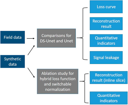
FIGURE 1. Scheme of the numerical experiments and analysis.

2 Theory and method

2.1 Loss function

The network training process updates network parameters using an optimizer according to the loss function. The suitable loss function can help to capture the intrinsic features of the inverse problem and speed up the convergence of the network (Huang et al., 2022). In this paper, we use a hybrid loss function (Yu and Wu, 2022) to obtain information from the missing part and global structure which is effective for seismic data reconstruction. The following describes the loss function used in this paper in detail.

1) $L_1$ loss function: Given the model prediction result $x$ and reference label data $y$, $L_1$ is calculated as

${Loss}_{L_1}=\frac{{\displaystyle \sum }_{i=1}^l{\displaystyle \sum }_{j=1}^m{\displaystyle \sum }_{k=1}^{n}w\left[i,j,k\right]\bullet \left|x\left[i,j,k\right]-y\left[i,j,k\right]\right|}{{\displaystyle \sum }_{i=1}^l{\displaystyle \sum }_{j=1}^m{\displaystyle \sum }_{k=1}^{n}w\left[i,j,k\right]},(1)$

where $x\left[i,j,k\right]$ and $y\left[i,j,k\right]$ are the seismic amplitude of $x$ and $y$, respectively; $l\bullet m\bullet n$ is the total number; and $w\left[i,j,k\right]$ represents a 3D binary mask which is equal to one at data missing position and zero elsewhere. Using $L_1$ as loss function makes the deep neural network pay more attention to recovering details of missing traces during training.

2) SSIM loss function: The structural similarity (SSIM) loss is used to capture the overall structural texture information of seismic data. SSIM is an indicator that measures the similarity between data, which is calculated from brightness, contrast, and structure (Wang et al., 2004). For the interpolation result of network output $x$ and corresponding labeled data $y$, the expression formula of $SSIM\left(x,y\right)$ is

$SSIM\left(x,y\right)=\frac{\left(2{\mu }_x{\mu }_y+c_1\right)\left(2{\sigma }_{xy}+c_2\right)}{\left({\mu }_x^2+{\mu }_y^2+c_1\right)\left({\sigma }_x^2+{\sigma }_y^2+c_2\right)},(2)$

where ${\mu }_x,{\mu }_y$ are the means; ${\sigma }_x,{\sigma }_y$ are the standard deviations; ${\sigma }_{xy}$ is the covariance; and $c_1,c_2$ are small constants. The value range of $SSIM\left(x,y\right)$ is $\left[\mathrm{0,1}\right]$; the closer to $1$, the more similar $x$ and $y$ is. We set the SSIM loss function as

${Loss}_{SSIM}=1-SSIM\left(x,y\right).(3)$

Since the calculation results of the two loss functions are in range $\left[\mathrm{0,1}\right]$, the hybrid loss function formula used in this paper is set as

${Loss}_{L_1+SSIM}={Loss}_{L_1}+{Loss}_{SSIM}.(4)$

Compared with the single loss function, the ${Loss}_{L_1+SSIM}$ captures both local and global information which is more suitable for the seismic missing trace reconstruction task (Yu and Wu, 2022).

2.2 Switchable normalization

We use switchable normalization ($SN$) (Luo et al., 2018) instead of batch normalization ($BN$) to eliminate the influence of minibatch size on $BN$ due to the increase of data dimension. The expression for switchable normalization is

$SN=w_{bn}\times BN+w_{in}\times IN+w_{\mathit{ln}}\times \mathit{LN},(5)$

where $IN$ is the instance normalization and $\mathit{LN}$ is the layer normalization. Since the mean and variance of $BN$ are calculated on a minibatch, the smaller the minibatch, the greater the noise generated by the estimation of this statistical information, which will lead to excessive regularization of model training and affect the generalization ability of the model. $IN$ and $\mathit{LN}$ are independent of the minibatch in calculation, but they cannot reach the accuracy of $BN$ due to the lack of regularization ability when the minibatch is large. $SN$ allows the network to learn the value of $w_{bn},w_{in},w_{\mathit{ln}}$ according to the data so that different normalization methods interact to overcome the aforementioned problems.

2.3 Depthwise separable convolution

Compared with 2D seismic data, the additional dimension of 3D seismic data can obtain more information from multi-dimension, which is beneficial for data interpolation. However, with the increasing dimensionality, the calculation operation of each component in the network will be greatly increased. Thus, we introduce depthwise separable convolution to replace standard convolution in some layers to reduce parameters and computation of the network. Depthwise separable convolution decomposes the standard convolution into two steps, namely, depthwise convolution and pointwise convolution. In the following, we first introduce the depthwise separable convolution on 2D data and then further introduce the depthwise separable convolution in the 3D case.

2.3.1 Convolution on 2D data

To make it easier to understand, we first introduce a simple example of using standard convolution and depthwise separable convolution, respectively, on 2D data, as shown in Figure 2. We assume that the 2D input data has 3 channels, and the size of the feature maps of each channel is $\mathrm{H}\times \mathrm{W}$. In addition, we use zero padding and the stride is set to 1 in both standard convolution and depthwise separable convolution. The following describes the process of these two kinds of convolution methods, as well as their parameter quantity and computation cost.

1) Standard convolution: As can be seen in Figure 2, $4$ convolution filters with the size of $3\times 3\times 3$ are directly applied to convolve the $3\times \mathrm{H}\times \mathrm{W}$ input data, and the output data are $4$ feature maps with the size of $\mathrm{H}\times \mathrm{W}$. The parameter quantity $P_{STD}$ and computation cost $C_{STD}$ required by the standard convolution are as follows:

$P_{STD}=4\times 3\times 3\times 3=108,(6)$

$C_{STD}=3\times 3\times H\times W\times 3\times 4=108\times H\times W.(7)$

2) Depthwise separable convolution: Unlike the standard convolution, the depthwise separable convolution is divided into two steps: depthwise convolution and pointwise convolution. It first uses depthwise convolutions to apply a single filter per input channel. Then, a simple 1×1 convolution named pointwise convolution is used to calculate a linear combination of the outputs of depthwise convolution for generating new features (Howard et al., 2017). For our 2D case in Figure 2, we first performed the depthwise convolution: applying $3$ convolution filters with the size of $3\times 3$ to the $3$ channels of $3\times \mathrm{H}\times \mathrm{W}$ input data, respectively, and obtaining $3$ feature maps with the size of $\mathrm{H}\times \mathrm{W}$. Then, we perform the pointwise convolution: $4$ convolution filters of size $1\times 1\times 3$ are applied to the $3$ feature maps obtained in the previous step, producing $4$ feature maps with the size of $\mathrm{H}\times \mathrm{W}$. The parameter quantity $P_{DS}$ and computation cost $C_{DS}$ required by the depthwise separable convolution are as follows:

$P_{DS}=3\times 3\times 3+1\times 1\times 3\times 4=39,(8)$

$C_{DS}=3\times H\times W\times 3\times 3+3\times 3\times 3\times 4=108+27\times H\times W.(9)$

FIGURE 2

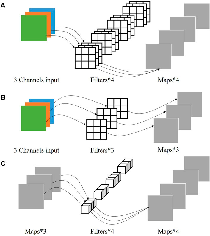
FIGURE 2. (A) Standard convolution; (B) depthwise convolution; and (C) pointwise convolution.

According to the aforementioned analysis, compared with standard convolution, depthwise separable convolution can effectively reduce the parameter and computation cost of the convolution layer, and the larger the size of input data is, the more parameter and computation cost are reduced. When dealing with practical problems, it often happens that the data size to be handled relies on the device hardware memory (GPU). The use of depthwise separable convolution can effectively mitigate this problem.

2.3.2 Convolution on 3D data

The input data in this paper is the 3D seismic data volume. In the training process, the input of convolution layers are usually 4D data with the size of $N\times H\times W\times D$, where $N$ is the number of channels and $H\times W\times D$ is the 3D feature map size. Based on the previous depthwise separable convolution for 2D data, we derive the depthwise separable convolution for 3D data used in this paper and compare it with the 3D standard convolution. Moreover, when applying depthwise separable convolution on 3D seismic data, we first conduct depthwise convolution along inline and crossline and then pointwise convolution along time axis. As shown in Figure 3, we assume that the 3D input data are a cube which has $N$ channels and the size of the feature map of each channel is $D_I\times D_I\times D_I$. Padding and stride are not specified in this 3D case.

1) Standard convolution: As shown in Figure 3, $M$ 3D convolution filters with the size of $D_k\times D_k\times D_k$ are directly applied to the $N\times D_I\times D_I\times D_I$ input data, producing the output data with the size of $M\times D_o\times D_o\times D_o$. The parameter quantity $P_{STD}$ and computation cost $C_{STD}$ in 3D standard convolution can be expressed as follows:

$P_{STD}=M\bullet D_k\bullet D_k\bullet D_k,(10)$

$C_{STD}=D_k\bullet D_k\bullet D_k\bullet N\bullet M\bullet D_I\bullet D_I\bullet D_I.(11)$

2) Depthwise separable convolution: Similar to the 2D case, $N$ convolution filters with size $1\times D_k\times D_k$ are first applied to the $N\times D_I\times D_I\times D_I$ input data for depthwise convolution, and a 3D feature map with $N$ channels and size of $D_o\times D_o\times D_I$ is obtained. Then, $M$ convolution filters with the size of $1\times 1\times D_k$ are used to perform pointwise convolution on the previously obtained feature map to produce the output data with the same size as the standard convolution. The parameter quantity $P_{DS}$ and computation cost $C_{DS}$ in depthwise separable convolution are:

$P_{DS}=N\bullet D_k\bullet D_k+M\bullet D_k,(12)$

$C_{DS}=D_k\bullet D_k\bullet N\bullet N\bullet D_I\bullet D_I\bullet D_I+D_k\bullet M\bullet N\bullet D_O\bullet D_O.(13)$

FIGURE 3

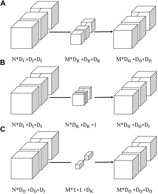
FIGURE 3. (A) Standard convolution; (B) depthwise convolution; and (C) pointwise convolution. $N,M$ are the channel number of input and output. $D_I,D_O,D_k$ are the spatial dimensions of input, output, and convolution kernels assumed to be square, respectively.

It can be concluded that the use of depthwise separable convolution can reduce the calculation workload of the network. The experimental part in this paper further verifies that the depthwise separable convolution can reduce the computation cost and parameter amount of 3D convolution neural network with close seismic data reconstruction results to standard convolution.

3 Network architecture

We design a 3D Unet network equipped with depthwise separable convolution for interpolation of 3D seismic data which coined as DS-Unet. In the experiment, we found that replacing all standard convolution with the depthwise separable convolution slows down the time of network training. Tan et al. (2021) pointed out that although the depthwise separable convolution greatly reduces the number of parameters, it divides the original one-step standard convolution into two steps, which increases the depth of the network and the intermediate variables that need to be saved and read. Then, a lot of time is spent on reading and writing data, resulting in slow training speed. Tan et al. (2021) addressed this problem by replacing the depthwise separable convolution in shallow layers with standard convolution. Likewise, in this paper, we use standard convolution in three layers close to the input and output of Unet, and use the depthwise separable convolution in the middle four layers. The underlying principle is that deeper layers have smaller feature maps, saving more time on reading and writing intermediate variables. The specific structural framework of the proposed network is shown in Figure 4.

FIGURE 4

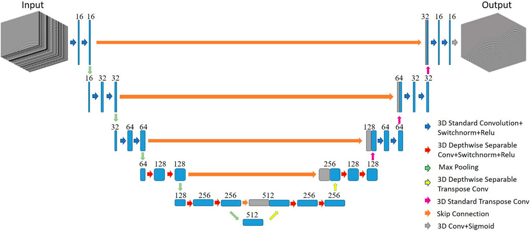
FIGURE 4. Architecture of DS-Unet. The left side is encoder, the right side is decoder, and the orange arrow in the middle is the jump connection layer. The red arrows and yellow arrows are depthwise separable convolution and Transpose convolution, respectively.

The construction of 3D Unet is to replace the 2D convolution, pooling, and up-sampling layers in 2D Unet with the corresponding 3D versions. Based on 3D Unet, our 3D DS-Unet entirely replaces the standard convolution (blue arrow) in the middle four layers with depthwise separable convolution (red and yellow arrow). Like the ordinary Unet, the input seismic data are first convolved and down sampled several times to obtain a feature map with 512 channels. This process is used to extract representative features of the input seismic data, which is called the encoder. Then, the feature map finally obtained by the encoder is convolved and up sampled for the same number of times to get the final result. This process is used to reconstruct the seismic data, which is called the decoder. In addition, the skip connection concatenates the feature maps of encoder layer and decoder layer to make up for the information lost in the down sampling process.

4 Experiments

4.1 Synthetic data

The synthetic dataset we used in the experiment is the SEG C3 dataset, which is a publicly available dataset, including 45 shots with 8 ms sample rate. Each shot has 201 × 201 receiver grids with 625 time samples per trace. We use the sliding window method to expand the data, selecting 1,710 cubes with the size of 128 × 128 × 128 from the whole dataset, of which 1,026 are used for training, 342 and 342 for validation and testing, respectively. Training, validation, and test dataset are extracted from shots with index number 1–27, 28–36, and 37–45, respectively, in order to ensure the generalization performance of the network. This ensures no overlapping on training, validation, and testing datasets. For each 128 × 128 × 128 cube, we randomly selected 30% traces in crossline direction and set the corresponding value to zero. We used the Adam optimization method with initial learning rate 0.001 in our paper. The number of training epochs is 25, and the batch size is 1. All network training in the experiments is implemented under the Pytorch framework, and GPU (GeForce RTX 2080 Ti) is used to speed up the computation.

Unet with standard convolution alone and DS-Unet with both standard and depthwise separable convolution are trained under the same conditions. We emphasize that both the models adopt hybrid loss function and switchable normalization, and the only difference between them is whether the depthwise separable convolution is used. The loss curves of two networks are shown in Figure 5; we can see that after 10 epochs, the training loss curves of the two models have coincided. For the validation loss, although the curves of the two models do not coincide, there is little difference, and the validation loss of DS-Unet even converges to a smaller value.

FIGURE 5

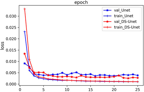
FIGURE 5. Loss curves of the two networks on the SEG C3 synthetic data.

Figure 6, Figures 7, and 8 are the time, inline, and crossline slices of the interpolation results obtained by the two networks on the SEG C3 synthetic dataset, respectively. The reconstruction results obtained by DS-Unet (Figure 6D, Figures 7D, 8D) are, in general, comparable with those obtained by Unet (Figure 6C, Figures 7C, 8C), and the different between them is almost indiscernible to the naked eye. Meanwhile, the results of the two models are very close to the ground truth (Figure 6B, Figures 7B, 8B).

FIGURE 6

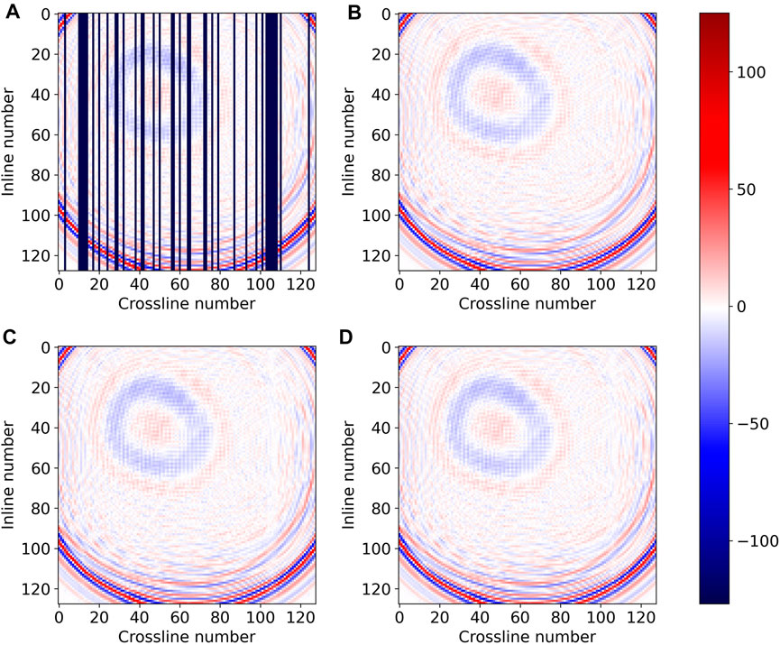
FIGURE 6. Time slice of interpolation results on the SEG C3 synthetic data: (A) missing traces data; (B) ground truth; (C) Unet (Chai et al., 2021); and (D) DS-Unet.

FIGURE 7

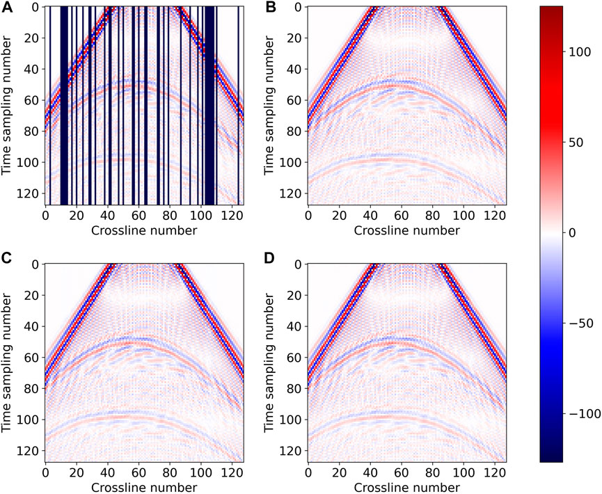
FIGURE 7. Inline slice of interpolation results on the SEG C3 synthetic data: (A) missing traces data; (B) ground truth; (C) Unet (Chai et al., 2021); and (D) DS-Unet.

FIGURE 8

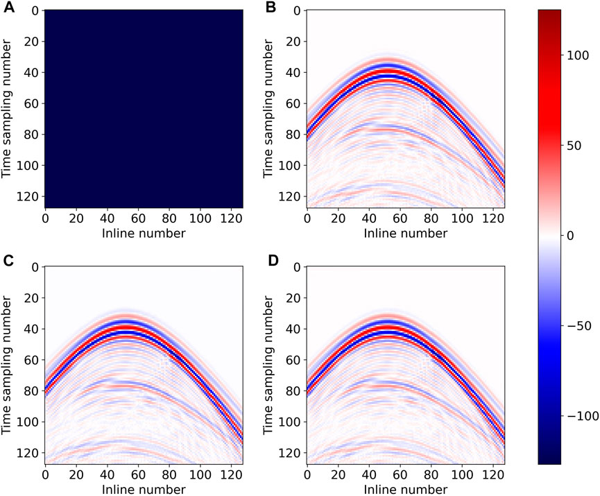
FIGURE 8. Crossline slice of interpolation results on the SEG C3 synthetic data: (A) (complete crossline) missing traces data; (B) ground truth; (C) Unet (Chai et al., 2021); and (D) DS-Unet.

To compare the interpolation results from a different perspective, we drew wiggle plots of crossline slice which display the reconstruction result of single trace, as shown in Figure 9. It is evident that the reconstruction result of Unet (Figure 9 left column) and DS-Unet (Figure 9 right column) represented by the black dashed line are very similar and almost coincide with the ground truth (red solid line). Inspecting these results, we can find that the reconstruction profiles obtained by our proposed DS-Unet are not significantly different from those obtained by Unet, and they are both close to the ground truth.

FIGURE 9

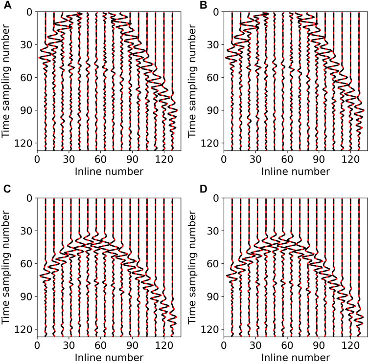
FIGURE 9. Wiggle plots on the SEG C3 synthetic data: (A) No.60 crossline slice of Unet; (B) No.60 crossline slice of DS-Unet, (C) No.110 crossline slice of Unet (Figure 8C), and (D) No.110 crossline slice of DS-Unet (Figure 8D); black dashed lines indicate reconstruction results and red solid line, ground truth.

To further compare the performance of the two models, we also calculated two quantitative indicators: MSE and SSIM, and the number of parameters and training time of the model, shown in Table 1. The interpolation results of the two networks are only slightly different in two metrics. However, comparing the number of parameters and training time of the model, the parameters of DS-Unet account for only 58% of Unet, which greatly reduces the memory usage of Unet. Moreover, the training time of DS-Unet is shortened by about 20% per epoch, compared to Unet. Experiments show that the DS-Unet can effectively reduce the operation cost of the network while maintaining the accuracy of network reconstruction results.

TABLE 1

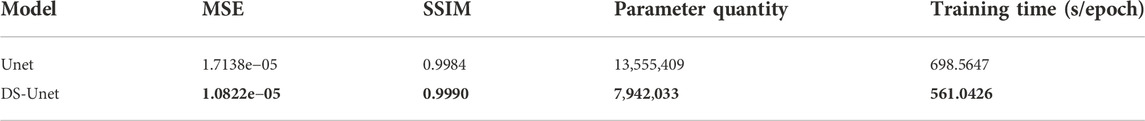
TABLE 1. Comparison of two networks on SEG C3 synthetic data (the bold font indicates the best value).

For better visualization and comparison, we draw the waveform of the interpolated traces and ground truth on 60th and 110th crosslines in Figure 9. As shown in Figure 10, the residual of interpolation results for the 110th crossline slice are presented. The left side of Figure 10 shows the residual of Unet, and the right side is that for DS-Unet; the SNR values are 19.1211 (Figure 10A), 23.7704 (Figure 10B), 19.5989 (Figure 10C), and 23.2223 (Figure 10D). Both the residual and SNR value show that signal leakage is more significant in the result of Unet compared to DS-Unet, indicating that DS-Unet has better reconstruction performance.

FIGURE 10

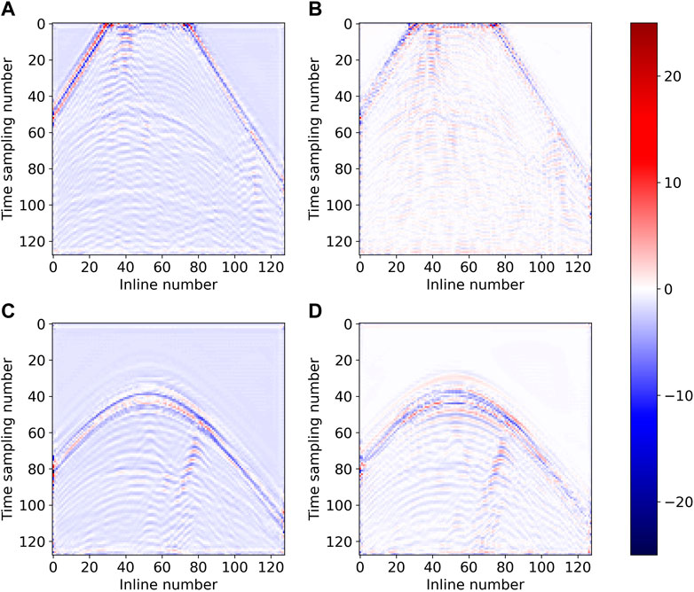
FIGURE 10. Residual of (A) Unet on No.60 crossline slice, (B) DS-Unet on No.60 crossline slice, (C) Unet on No.110 crossline slice (Figure 8C), and (D) DS-Unet on No.110 crossline slice (Figure 8D).

4.2 Field data

The experiment on field data is conducted on Mobil AVO Viking graben line 12, which is a public dataset composed of 1,001 shots. Each shot has 120 traces, and each trace has 1,500 samples. The time sampling interval and space sampling interval are 4 ms and 25 m, respectively. It is worth noting that although the dataset is 2D profile, it can be regarded as 3D data composed of three dimensions: shot position, receiver position, and time. A similar processing can be seen in the study by Chai et al. (2021), which also treated this 2D field seismic data as 3D data for 3D seismic data interpolation tests. We still use the sliding window method to divide the whole 3D data volume into a large number of small cubes to expand the training samples. Additionally, the size of each cube is set to 96 × 96 × 96. We perform the sliding window method on the first 600 shots to obtain 1,092 cubes as training samples, and perform the same operation on the subsequent 400 shots to obtain 504 samples, 252 of which are taken as the validation dataset and others as test dataset. Traces are still 30% randomly missing in the receiver direction. We test the performance of DS-Unet and Unet on this field dataset. Except for the number of epochs which is set to 30, other hyperparameter settings and training conditions are same as those of the experiment of synthetic data.

Figure 11 shows the convergence curves of DS-Unet and Unet. It can be observed that although the training loss of Unet finally converges to a smaller value, the difference between the training losses of the two models are both very small after 20 epochs. In addition, for validation loss curves, the two models almost coincide after 20 epochs.

FIGURE 11

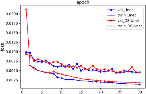
FIGURE 11. Loss curves of the two networks on field data.

Figures 12–14 compare the reconstruction results of the two models in three dimensions: time, shot position, and receiver position. Figures 12C–13C–14C and Figures 12D–13D–14D show the seismic data reconstructed by Unet and DS-Unet in three dimensions, respectively. It can be observed that they are very close to the ground truth (Figures 12B–13B–14B), indicating both models can achieve good interpolation results. Further comparing the reconstruction results of the two models, we can find that the differences between them are visually undetectable in the three dimension slices. In conclusion, DS-Unet with depthwise separable convolution reduces the memory and computation required when training the network and achieves comparable interpolation accuracy as Unet.

FIGURE 12

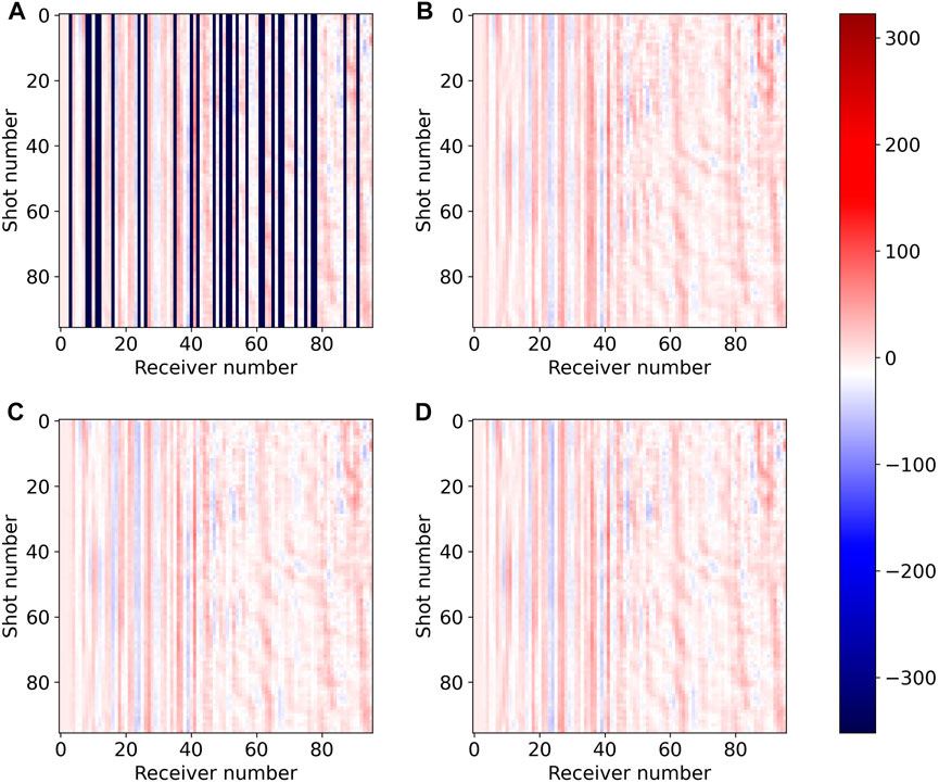
FIGURE 12. Time slice of interpolation results on field data: (A) missing traces data, (B) ground truth, (C) Unet (Chai et al., 2021), and (D) DS-Unet.

FIGURE 13

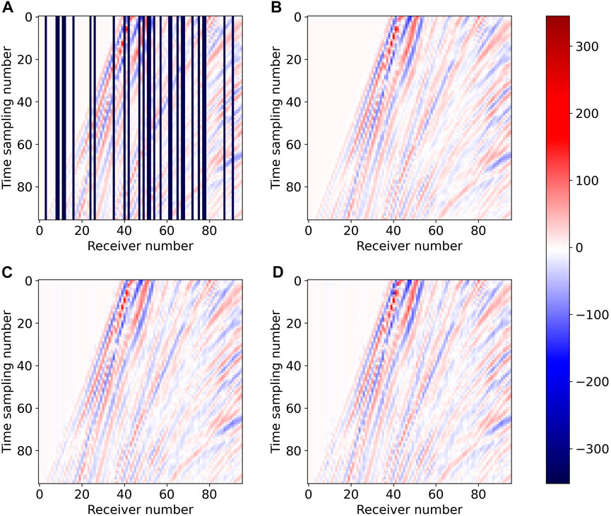
FIGURE 13. Shot slice of interpolation results on field data: (A) missing traces data, (B) ground truth, (C) Unet (Chai et al., 2021), and (D) DS-Unet.

FIGURE 14

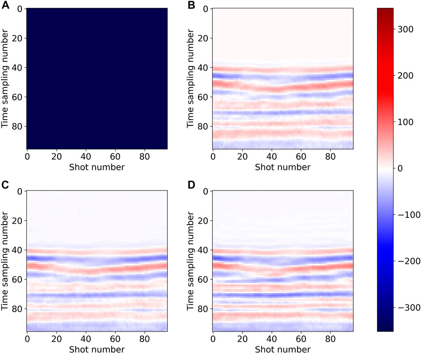
FIGURE 14. Receiver slice of interpolation results on field data: (A) (complete receiver) missing traces data, (B) ground truth, (C) Unet (Chai et al., 2021), and (D) DS-Unet.

In addition, we also drew wiggle plots of common receiver gather, that is, plot seismic trace with a fixed receiver number for different shots to compare the reconstruction results of single seismic trace, shown in Figure 15. It indicates that the reconstructed seismic data of the two models represented by the black dashed line well fit the real seismic data represented by the red solid line.

FIGURE 15

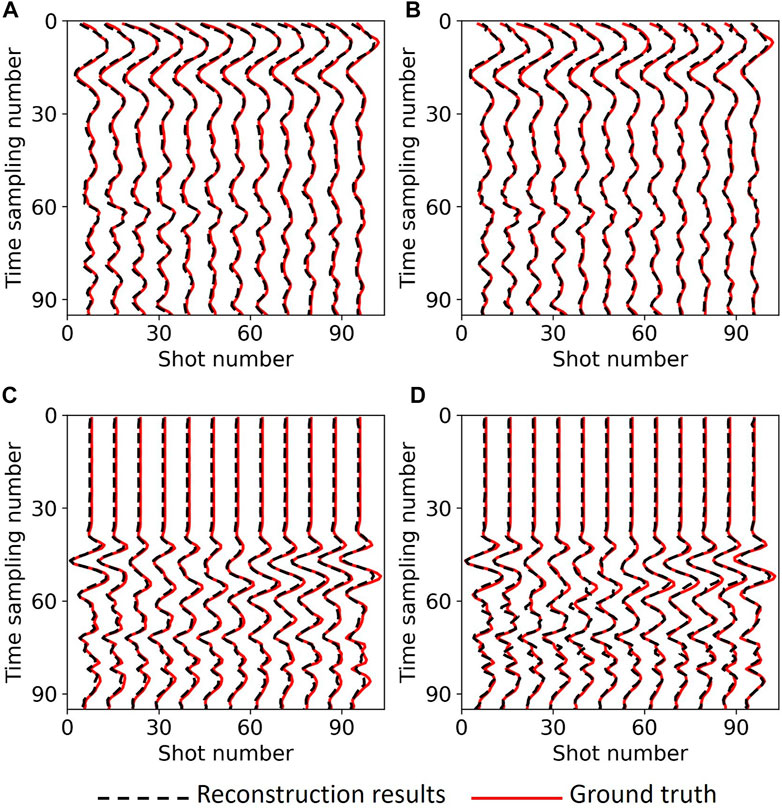
FIGURE 15. Wiggle plots on field data: (A) No.49 receiver slice of Unet, (B) No.49 receiver slice of DS-Unet, (C) No.24 receiver slice of Unet (Figure 14C), and (D) No.24 receiver slice of DS-Unet (Figure 14D); black dashed lines indicate reconstruction results, and red solid line, ground truth.

Quantitative indicators are shown in Table 2. Comparing MSE and SSIM in the table, it can be seen that Unet outperforms DS-Unet by small margins. However, the parameter quantity and training time of DS-Unet are significantly decreased compared to Unet, which are reduced by 40% and 13%, respectively. Therefore, although DS-Unet using depthwise separable convolution has performance similar to Unet using standard convolution alone, DS-Unet is superior to Unet in terms of both memory and time.

TABLE 2

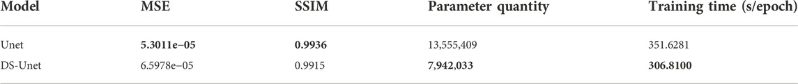
TABLE 2. Comparison of two networks on field data (the bold font indicates the best value).

Figure 16 is the residual corresponding to Figure 15. We can see that for the 49th receiver (the first row of Figure 16), the residual of Unet (Figure 16A) is not very different from DS-Unet (Figure 16B), and the SNR values are also very close, which are 11.5034 and 11.1270, respectively. There is no significant difference in signal leakage between them. For the 24th receiver (the second row of Figure 16), the residual of Unet (Figure 16C) is with smaller amplitude than DS-Unet (Figure 16D), and the SNR values are 8.6916 and 6.6798, respectively, which are not very different from each other. Additionally, we think such a gap is acceptable compared with the significant advantage of DS-Unet in the number of parameters and calculation.

FIGURE 16

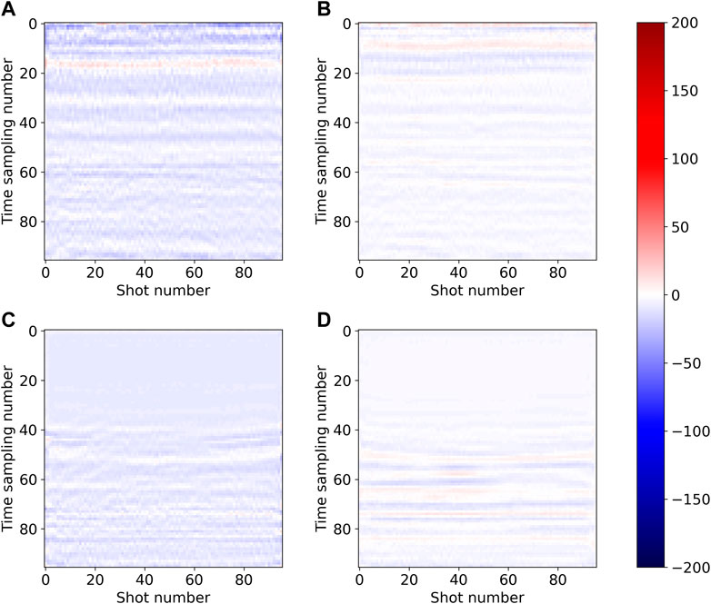
FIGURE 16. Residual of (A) Unet on No.49 receiver slice, (B) DS-Unet on No.49 receiver slice, (C) Unet on No.24 receiver slice (Figure 14C), and (D) DS-Unet on No.24 receiver slice (Figure 14D).

4.3 Ablation study

In order to further illustrate the improvement of interpolation results by hybrid loss and switchable normalization, we conduct ablation experiments on the SEG C3 synthetic dataset. The network structure used in the experiments is DS-Unet. The results are shown in Figure 17 and Table 3. Figure 17C shows the interpolation results of the model using the MSE loss function, with more detail missing and notable white bar artifacts in the red box compared to Figure 17E, which is the result of the model using hybrid loss function. The interpolation result using batch normalization (Figure 17D) also has evident line-like artifacts in the blue box, with poor continuity. Table 3 shows the quantitative evaluation indicators of the interpolation results. The MSE indicator of the model using batch normalization is 20.5329e−05, which is more than three times worse than that of the model using switchable normalization, indicating that using batch normalization instead of switchable normalization will significantly degrade the interpolation performance of the model. Additionally, from the the second and third rows in Table 3, we can conclude that the hybrid loss function has better interpolation effect than the MSE loss function. In summary, the model using both the hybrid loss function and switchable normalization performs best in both the MSE and SSIM indicator, and it is also closest to the ground truth in Figure 17B.

FIGURE 17

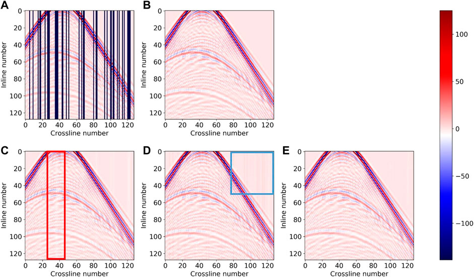
FIGURE 17. Interpolation results using different loss functions and normalization methods on the SEG C3 synthetic data: (A) missing traces data, (B) ground truth, (C) swichnorm+MSE loss, (D) batchnorm+hybrid loss, and (E) swichnorm+hybrid loss.

TABLE 3

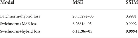
TABLE 3. Ablation experiment on SEG C3 synthetic data (the bold font indicates the best value).

5 Discussion

Deep learning has been widely used in seismic data processing. However, for high-dimensional seismic data, they are often limited by computer memory due to the huge number of parameters. To solve this problem, we propose DS-Unet, which replaces the standard convolution with the depthwise separable convolution in some layers of Unet, so that the number of parameters and computation can be greatly reduced while ensuring the accuracy of interpolation results. It is worth noting that we did not replace all the standard convolution in Unet with the depthwise separable convolution. Standard convolution is still used in the shallow layers of DS-Unet. However, determining which layer can use the depthwise separable convolution is not discussed in depth in this work, and we believe that there is still much room for exploration. The method proposed in this paper is relatively simple, but we think depthwise separable convolution may better show its advantages in more complex network architectures, which is also one of the directions we will explore in the future. Moreover, we only conduct experiments on irregular missing cases. For other more complex missing cases, such as consecutive missing, our proposed method is difficult to achieve a good interpolation effect. In the future, we will explore other effective network architectures to reconstruct complex missing seismic data. Finally, the depthwise separable convolution may be extended to the unsupervised seismic data interpolation/denoising and also other tasks to reduce the parameter and computation cost without degradation results.

6 Conclusion

In this paper, we propose an interpolation method for 3D irregular missing seismic data. Using the depthwise separable convolution, the quantity of parameters and computation cost of the network can be reduced, so that the network becomes more lightweight. Experiments on synthetic data and field data show that the convergence trend of loss curves of DS-Unet and Unet is very similar and finally converges to almost the same value. Additionally, the difference between the interpolation results of the two models in three different dimension slices is visually undetectable. For better evaluation, we calculate the values of two quantitative indicators. They are slightly different in the two datasets: DS-Unet performs better on the synthetic data set, but on the field data, we find that Unet performs better. However, no matter which dataset, the difference of quantitative indicators between the two models is very small. The advantage of DS-Unet is that it requires less parameters and calculation. Compared with Unet, it reduces the number of parameters by about 40%, and the training time for the two datasets is also reduced to varying degrees. The aforementioned results indicate that the proper use of the depthwise separable convolution can significantly improve operation efficiency and reduce the required parameters on the premise of ensuring the reconstruction accuracy. We also use the hybrid loss function ${Loss}_{L_1+SSIM}$ and switchable normalization to further improve the reconstruction results, and ablation study shows that they make the interpolation results more detailed and reduce artifacts.

Data availability statement

Publicly available datasets are analyzed in this study. These data can be found here: https://wiki.seg.org/wiki/SEG_C3_45_shot, https://wiki.seg.org/wiki/Mobil_AVO_viking_graben_line_12.

Author contributions

BW, ZJ, and XL contributed to the conception of the study. Writing, compiling, and debugging of the program were completed by ZJ and XL. XL wrote the first draft of the manuscript, and all authors contributed to the revision.

Funding

This work was supported by the National Natural Science Foundation of China under Grant 41974122 and the Guangdong Provincial Key Laboratory of Geophysical High-resolution Imaging Technology (2022B1212010002).

Acknowledgments

The authors express sincere thanks to the Sandia National Laboratory and Mobil Oil Company for open data.

Conflict of interest

The authors declare that the research was conducted in the absence of any commercial or financial relationships that could be construed as a potential conflict of interest.

Publisher’s note

All claims expressed in this article are solely those of the authors and do not necessarily represent those of their affiliated organizations, or those of the publisher, the editors, and the reviewers. Any product that may be evaluated in this article, or claim that may be made by its manufacturer, is not guaranteed or endorsed by the publisher.

References

Alaei, N., Roshandel Kahoo, A., Kamkar Rouhani, A., and Soleimani, M. (2018). Seismic resolution enhancement using scale transform in the time-frequency domain. Geophysics 83 (6), V305–V314. doi:10.1190/geo2017-0248.1

CrossRef Full Text | Google Scholar

Anvari, R., Mohammadi, M., and Kahoo, A. R. (2018). Enhancing 3-D seismic data using the t-SVD and optimal shrinkage of singular value. IEEE J. Sel. Top. Appl. Earth Obs. Remote Sens. 12 (1), 382–388. doi:10.1109/jstars.2018.2883404

CrossRef Full Text | Google Scholar

Anvari, R., Mohammadi, M., Kahoo, A. R., Khan, N. A., and Abdullah, A. I. (2020). Random noise attenuation of 2D seismic data based on sparse low-rank estimation of the seismic signal. Comput. Geosciences 135, 104376. doi:10.1016/j.cageo.2019.104376

CrossRef Full Text | Google Scholar

Beheshti, N., and Johnsson, L. (2020). “Squeeze u-net: A memory and energy efficient image segmentation network,” in Proceedings of the IEEE/CVF conference on computer vision and pattern recognition workshops, Seattle, WA, United States, June 2020, 364

CrossRef Full Text | Google Scholar

Chai, X., Gu, H., Li, F., Duan, H., Hu, X., and Lin, K. (2020). Deep learning for irregularly and regularly missing data reconstruction. Sci. Rep. 10 (1), 3302–3318. doi:10.1038/s41598-020-59801-x

PubMed Abstract | CrossRef Full Text | Google Scholar

Chai, X., Tang, G., Wang, S., Lin, K., and Peng, R. (2021). Deep learning for irregularly and regularly missing 3-D data reconstruction. IEEE Trans. Geosci. Remote Sens. 59 (7), 6244–6265. doi:10.1109/tgrs.2020.3016343

CrossRef Full Text | Google Scholar

Farrokhnia, F., Kahoo, A. R., and Soleimani, M. (2018). Automatic salt dome detection in seismic data by combination of attribute analysis on CRS images and IGU map delineation. J. Appl. Geophys. 159, 395–407. doi:10.1016/j.jappgeo.2018.09.018

CrossRef Full Text | Google Scholar

Ferdian, E., Suinesiaputra, A., Dubowitz, D. J., Zhao, D., Wang, A., Cowan, B., et al. (2020). 4DFlowNet: Super-resolution 4D flow MRI using deep learning and computational fluid dynamics. Front. Phys. 138. doi:10.3389/fphy.2020.00138

CrossRef Full Text | Google Scholar

Gadosey, P. K., Li, Y., Agyekum, E. A., Zhang, T., Liu, Z., Yamak, P. T., et al. (2020). SD-UNET: Stripping down U-net for segmentation of biomedical images on platforms with low computational budgets. Diagnostics 10 (2), 110. doi:10.3390/diagnostics10020110

PubMed Abstract | CrossRef Full Text | Google Scholar

Gholtashi, S., Nazari Siahsar, M. A., RoshandelKahoo, A., Marvi, H., and Ahmadifard, A. (2015). Synchrosqueezing-based transform and its application in seismic data analysis. Iran. J. Oil Gas Sci. Technol. 4 (4), 1–14.

Google Scholar

Hosseini-Fard, E., Roshandel-Kahoo, A., Soleimani-Monfared, M., Khayer, K., and Ahmadi-Fard, A. R. (2022). Automatic seismic image segmentation by introducing a novel strategy in histogram of oriented gradients. J. Petroleum Sci. Eng. 209, 109971. doi:10.1016/j.petrol.2021.109971

CrossRef Full Text | Google Scholar

Howard, A. G., et al. (2017). Mobilenets: Efficient convolutional neural networks for mobile vision applications. https://arxiv.org/abs/1704.04861.

Google Scholar

Huang, H., Wang, T., Cheng, J., Xiong, Y., Wang, C., and Geng, J. (2022). Self-Supervised deep learning to reconstruct seismic data with consecutively missing traces. IEEE Trans. Geosci. Remote Sens. 60, 1–14. doi:10.1109/TGRS.2022.3148994

CrossRef Full Text | Google Scholar

Huang, W., and Liu, J. (2020). Robust seismic image interpolation with mathematical morphological constraint. IEEE Trans. Image Process. 29, 819–829. doi:10.1109/tip.2019.2936744

CrossRef Full Text | Google Scholar

Huang, W. (2022). Seismic data interpolation by Shannon entropy-based shaping. IEEE Trans. Geosci. Remote Sens. 60, 1–12. doi:10.1109/tgrs.2022.3180200

CrossRef Full Text | Google Scholar

Jia, Y., and Ma, J. (2017). What can machine learning do for seismic data processing? An interpolation application. Geophysics 82 (3), 163–177. doi:10.1190/geo2016-0300.1

CrossRef Full Text | Google Scholar

Jiang, J., Ren, H., and Zhang, M. (2022). A convolutional autoencoder method for simultaneous seismic data reconstruction and denoising. IEEE Geosci. Remote Sens. Lett. 19, 1–5. doi:10.1109/lgrs.2021.3073560

CrossRef Full Text | Google Scholar

Kahoo, A. R., Soleimani Monfared, M., and Radad, M. (2021). Identification and modeling of salt dome in seismic data using three-dimensional texture gradient. Iran. J. Geophys. 15 (1), 19. doi:10.30499/IJG.2020.242349.1285

CrossRef Full Text | Google Scholar

Khasraji Nejad, H., Kahoo, A. R., Soleimani Monfared, M., Radad, M., and Khayer, K. (2021). Proposing a new strategy in multi seismic attribute combination for identification of buried channel. Mar. Geophys. Res. 42, 35. doi:10.1007/s11001-021-09458-6

CrossRef Full Text | Google Scholar

Khayer, K., Roshandel Kahoo, A., Soleimani Monfared, M., Tokhmechi, B., and Kavousi, K. (2022). Target-Oriented fusion of attributes in data level for salt dome geobody delineation in seismic data. Nat. Resour. Res. 31, 2461–2481. doi:10.1007/s11053-022-10086-z

CrossRef Full Text | Google Scholar

Khayer, K., Roshandel-Kahoo, A., Soleimani-Monfared, M., and Kavoosi, K. (2022). Combination of seismic attributes using graph-based methods to identify the salt dome boundary. J. Petroleum Sci. Eng. 215, 110625. doi:10.1016/j.petrol.2022.110625

CrossRef Full Text | Google Scholar

Kong, F., Picetti, F., Lipari, V., Bestagini, P., Tang, X., and Tubaro, S. (2022). Deep prior-based unsupervised reconstruction of irregularly sampled seismic data. IEEE Geosci. Remote Sens. Lett. 19, 1–5. doi:10.1109/lgrs.2020.3044455

CrossRef Full Text | Google Scholar

Li, H., Lin, J., Wu, B., Gao, J., and Liu, N. (2022). Elastic properties estimation from prestack seismic data using GGCNNs and application on tight sandstone reservoir characterization. IEEE Trans. Geosci. Remote Sens. 60, 1–21. doi:10.1109/tgrs.2021.3079963

CrossRef Full Text | Google Scholar

Li, X., Wu, B., Zhu, X., and Yang, H. (2022). Consecutively missing seismic data interpolation based on coordinate attention unet. IEEE Geosci. Remote Sens. Lett. 19, 1–5. doi:10.1109/lgrs.2021.3128511

CrossRef Full Text | Google Scholar

Li, Y., Zhao, J., Lv, Z., and Pan, Z. (2021). Multimodal medical supervised image fusion method by CNN. Front. Neurosci. 303, 638976. doi:10.3389/fnins.2021.638976

PubMed Abstract | CrossRef Full Text | Google Scholar

Lin, L., Zhong, Z., Cai, Z., Sun, A. Y., and Li, C. (2022). Automatic geologic fault identification from seismic data using 2.5 D channel attention U-net. Geophysics 87 (4), IM111–IM124. doi:10.1190/geo2021-0805.1

CrossRef Full Text | Google Scholar

Liu, Q., Fu, L., and Zhang, M. (2021). Deep-seismic-prior-based reconstruction of seismic data using convolutional neural networks. Geophysics 86 (2), V131–V142. doi:10.1190/geo2019-0570.1

CrossRef Full Text | Google Scholar

Luo, P., Ren, J., Peng, Z., Zhang, R., and Li, J. (2018). Differentiable learning-to-normalize via switchable normalization. https://arxiv.org/abs/1806.10779.

Google Scholar

Mahdavi, A., Kahoo, A. R., Radad, M., and Monfared, M. S. (2021). Application of the local maximum synchrosqueezing transform for seismic data. Digit. Signal Process. 110, 102934. doi:10.1016/j.dsp.2020.102934

CrossRef Full Text | Google Scholar

Mandelli, S., Borra, F., Lipari, V., Bestagini, P., Sarti, A., and Tubaro, S. (2018). Seismic data interpolation through convolutional autoencoder. SEG Tech. Program Expand. Abstr. 2018. Soc. Explor. Geophys. 12, 4101–4105. doi:10.1190/segam2018-2995428.1

CrossRef Full Text | Google Scholar

Manor, R., and Geva, A. B. (2015). Convolutional neural network for multi-category rapid serial visual presentation BCI. Front. Comput. Neurosci. 9, 146. doi:10.3389/fncom.2015.00146

PubMed Abstract | CrossRef Full Text | Google Scholar

Oliveira, D. A., Ferreira, R. S., Silva, R., and Brazil, E. V. (2018). Interpolating seismic data with conditional generative adversarial networks. IEEE Geosci. Remote Sens. Lett. 15 (12), 1952–1956. doi:10.1109/lgrs.2018.2866199

CrossRef Full Text | Google Scholar

Qi, K., Yang, H., Li, C., Liu, Z., Wang, M., Liu, Q., et al. (2019). “X-net: Brain stroke lesion segmentation based on depthwise separable convolution and long-range dependencies,” in International conference on medical image computing and computer-assisted intervention, Shenzhen, Guangdong Province, China, October 2019 (Springer), 247

CrossRef Full Text | Google Scholar

Qiu, C., Wu, B., Liu, N., Zhu, X., and Ren, H. (2022). Deep learning prior model for unsupervised seismic data random noise attenuation. IEEE Geosci. Remote Sens. Lett. 19, 1–5. doi:10.1109/lgrs.2021.3053760

CrossRef Full Text | Google Scholar

Rao, P. K., and Chatterjee, S. (2021). Wp-unet: Weight pruning u-net with depthwise separable convolutions for semantic segmentation of kidney tumors.

Google Scholar

Shahbazi, A., Monfared, M. S., Thiruchelvam, V., Fei, T. K., and Babasafari, A. A. (2020). Integration of knowledge-based seismic inversion and sedimentological investigations for heterogeneous reservoir. J. Asian Earth Sci. 202, 104541. doi:10.1016/j.jseaes.2020.104541

CrossRef Full Text | Google Scholar

Siahsar, M. A. N., Gholtashi, S., Abolghasemi, V., and Chen, Y. (2017). Simultaneous denoising and interpolation of 2D seismic data using data-driven non-negative dictionary learning. Signal Process. 141, 309–321. doi:10.1016/j.sigpro.2017.06.017

CrossRef Full Text | Google Scholar

Soleimani, M., Aghajani, H., and Heydari-Nejad, S. (2018). Structure of giant buried mud volcanoes in the South Caspian Basin: Enhanced seismic image and field gravity data by using normalized full gradient method. Interpretation 6 (4), T861–T872. doi:10.1190/int-2018-0009.1

CrossRef Full Text | Google Scholar

Soleimani, M. (2017). Challenges of seismic imaging in complex media around Iran, from Zagros overthrust in the southwest to Gorgan Plain in the northeast. Lead. Edge 36 (6), 499–506. doi:10.1190/tle36060499.1

CrossRef Full Text | Google Scholar

Soleimani, M. (2016). Seismic imaging by 3D partial CDS method in complex media. J. Petroleum Sci. Eng. 143, 54–64. doi:10.1016/j.petrol.2016.02.019

CrossRef Full Text | Google Scholar

Soleimani, M. (2015). Seismic imaging of mud volcano boundary in the east of Caspian Sea by common diffraction surface stack method. Arab. J. Geosci. 8 (6), 3943–3958. doi:10.1007/s12517-014-1497-5

CrossRef Full Text | Google Scholar

Tan, M., and Le, Q. (2021). Efficientnetv2: Smaller models and faster training. Proc. 38th Int. Conf. Mach. Learn. PMLR 139, 10096

Google Scholar

Tavoosi, J., Zhang, C., Mohammadzadeh, A., Mobayen, S., and Mosavi, A. H. (2021). Medical image interpolation using recurrent type-2 fuzzy neural network. Front. Neuroinform. 15, 667375. doi:10.3389/fninf.2021.667375

PubMed Abstract | CrossRef Full Text | Google Scholar

Wang, Z., Bovik, A. C., Sheikh, H. R., and Simoncelli, E. P. (2004). Image quality assessment: From error visibility to structural similarity. IEEE Trans. Image Process. 13 (4), 600–612. doi:10.1109/tip.2003.819861

PubMed Abstract | CrossRef Full Text | Google Scholar

Wang, Z., Li, B., Liu, N., Wu, B., and Zhu, X. (2022). Distilling knowledge from an ensemble of convolutional neural networks for seismic fault detection. IEEE Geosci. Remote Sens. Lett. 19, 1–5. doi:10.1109/LGRS.2020.3034960

CrossRef Full Text | Google Scholar

Wei, Q., Li, X., and Song, M. (2021). De-aliased seismic data interpolation using conditional Wasserstein generative adversarial networks. Comput. Geosciences 154, 104801. doi:10.1016/j.cageo.2021.104801

CrossRef Full Text | Google Scholar

Wu, B., Meng, D., Wang, L., Liu, N., and Wang, Y. (2020). Seismic impedance inversion using fully convolutional residual network and transfer learning. IEEE Geosci. Remote Sens. Lett. 17 (12), 2140–2144. doi:10.1109/lgrs.2019.2963106

CrossRef Full Text | Google Scholar

Wu, X., Liang, L., Shi, Y., and Fomel, S. (2019). FaultSeg3D: Using synthetic data sets to train an end-to-end convolutional neural network for 3D seismic fault segmentation. Geophysics 84 (3), IM35–IM45. doi:10.1190/geo2018-0646.1

CrossRef Full Text | Google Scholar

Yang, L., Chen, W., Wang, H., and Chen, Y. (2021). Deep learning seismic random noise attenuation via improved residual convolutional neural network. IEEE Trans. Geosci. Remote Sens. 59 (9), 7968–7981. doi:10.1109/tgrs.2021.3053399

CrossRef Full Text | Google Scholar

Yang, L., Wang, S., Chen, X., Saad, O. M., Chen, W., Oboué, Y. A. S. I., et al. (2022). Unsupervised 3-D random noise attenuation using deep skip autoencoder. IEEE Trans. Geosci. Remote Sens. 60, 1–16. doi:10.1109/tgrs.2021.3100455

CrossRef Full Text | Google Scholar

Yoon, D., Yeeh, Z., and Byun, J. (2021). Seismic data reconstruction using deep bidirectional long short-term memory with skip connections. IEEE Geosci. Remote Sens. Lett. 18 (7), 1298–1302. doi:10.1109/lgrs.2020.2993847

CrossRef Full Text | Google Scholar

Yu, J., and Wu, B. (2022). Attention and hybrid loss guided deep learning for consecutively missing seismic data reconstruction. IEEE Trans. Geosci. Remote Sens. 60, 1–8. doi:10.1109/tgrs.2021.3068279

CrossRef Full Text | Google Scholar

Zabihi, S., Rahimian, E., Asif, A., and Mohammadi, A. (2021). “SepUnet: Depthwise separable convolution integrated U-net for MRI reconstruction,” in 2021 IEEE International Conference on Image Processing (ICIP), Berkeley, United States, June 2021, 3792

CrossRef Full Text | Google Scholar

Zhang, X., Zheng, Y., Liu, W., Peng, Y., and Wang, Z. (2020). An improved architecture for urban building extraction based on depthwise separable convolution. J. Intelligent Fuzzy Syst. 38 (5), 5821–5829. doi:10.3233/jifs-179669

CrossRef Full Text | Google Scholar

Zhu, D., Li, L., Guo, R., Tao, C., and Zhan, S. (2022). 3D fault detection: Using human reasoning to improve performance of convolutional neural networks. Geophysics 87 (4), IM143–IM156. doi:10.1190/geo2020-0905.1

CrossRef Full Text | Google Scholar