An optimized three-dimensional time-space domain staggered-grid finite-difference method

Numerical simulation of three-dimensional (3D) seismic wavefields forms the basis of the research on the migration methods of 3D seismic data based on wave equations. Because the simulation precision of wavefield extrapolation determines the imaging accuracy to a certain extent, it is very important to study how to enhance the forward modeling precision of 3D seismic wavefields. Thus, we build on an optimized 3D staggered-grid finite-difference (SFD) method with high simulation precision based on two-dimensional (2D) seismic modeling. Since it generates the corresponding difference coefficients by utilizing the least square (LS) method to minimize the objective function constructed by the time-space domain dispersion relation of the 3D acoustic wave equation, our optimized time-space domain LS-based 3D SFD method can effectively enhance the modeling precision of the 3D seismic wavefields in theory compared with the 3D SFD methods based on the Taylor-series expansion (TE), especially for the large wavenumber range. Examining the numerical dispersion, algorithm stability and computational cost, we compare our optimized time-space domain LS-based 3D SFD method with three conventional TE-based and LS-based 3D SFD methods to illustrate and demonstrate its effectiveness and feasibility. The numerical examples from different 3D models suggest that our optimized time-space domain LS-based 3D SFD method can generate less numerical dispersion and higher simulation accuracy for 3D seismic wavefields than three other conventional 3D SFD methods, but its stability condition is stricter and its computational cost is slightly higher.

Introduction

In recent years, the 3D seismic exploration has become one of the main methods to improve the recognition capacity for underground complex geological structures. As the key procedure of 3D seismic data processing, the numerical modeling of 3D seismic wavefields is the basis of the research on the migration methods based on two-way wave equations, because the wavefield extrapolation, which is essentially wavefield numerical modeling, is the core algorithm of this kind of imaging methods. At present, three different approaches are frequently used to solve the different wave equations to model the response characteristics of seismic wave in different media, such as pseudospectral methods (Fornberg, 1987; Huang et al., 2010; Alkhalifah, 2013), finite-element methods (Teng and Dai, 1989; Sotelo et al., 2021), and finite-difference (FD) methods (Bartolo et al., 2012; Fan et al., 2017; Wang et al., 2019a; Wang et al., 2019b; Wang et al., 2021). Among above three approaches, the FD methods are extensively used in the process of seismic modeling compared with the other two methods because of its simple principle, high implementation efficiency and low computational cost. Over the last few decades, the FD methods have been extensively investigated in different aspects, especially the 2D FD methods. For 3D FD methods, the existing conventional FD methods usually cannot meet the requirements of fast and high precision imaging, and therefore it is important to explore how to effectively enhance the precision of 3D seismic modeling for the 3D migration methods based on wave equations.

A focal point of the study of FD methods is to improve the numerical simulation precision, and there are many strategies to achieve this goal. For example, the SFD methods (Virieux, 1984; Virieux, 1986; Robertsson, 1996; Yang et al., 2017; Liang et al., 2018) have a higher modeling precision compared to the conventional FD methods, and therefore the SFD methods are more commonly used than the FD methods for improving the numerical simulation accuracy of seismic wavefields. There is another strategy to achieve this goal effectively: high-order FD or SFD schemes and its corresponding optimal difference coefficients. For this reason, the FD and SFD methods have been deeply explored to obtain high-order simulation precision for temporal and spatial partial derivatives in recent years (Ren and Li, 2019). Correspondingly, the calculation approaches of its difference coefficients have also been systematically discussed in the past few decades, and there are two frequently-used strategies: one is to optimize the objective functions constructed by the space domain dispersion relations (Dablain, 1986; Liu, 2014) and the other is to optimize the objective functions constructed by the time-space domain dispersion relations (Liu and Sen, 2009a; Liu and Sen, 2011a; Liu and Sen, 2011b, Liu and Sen, 2013; Wang et al., 2014; Cai et al., 2015; Ren and Liu, 2015; Xu and Liu, 2018). Using different optimization algorithms to deal with the objective functions of two dispersion relations, such as the TE method (Liu and Sen, 2009b; Liu and Sen, 2011a; Ren and Li, 2017) or LS method (Liu, 2013; Liu, 2014; Ren and Liu, 2015; Xu et al., 2019; Liu et al., 2021), a variety of difference coefficients can be correspondingly generated to simulate seismic wavefields at different times with different simulation accuracy, and therefore they can be called as the different FD or SFD methods. For example, there is a common naming strategy that have been extensively discussed in different publications, including the space domain or time-space domain TE-based methods (Liu and Sen, 2009a; Liu and Sen, 2011a) and the space domain or time-space domain LS-based methods (Liu, 2013; Liu, 2014; Ren and Liu, 2015). In the above four methods, the time-space domain methods usually have higher simulation accuracy than the space domain methods and the LS-based methods usually have higher simulation accuracy than the TE-based methods, which has been fully verified in 2D seismic modeling.

For the numerical simulation of 3D seismic wavefields, different scholars have also done a lot of work in the above different aspects according to 2D FD and SFD methods (Yomogida and Etgen, 1993; Robertsson et al., 1994; Graves, 1996; Pitarka, 1999; Etgen and O’Brien, 2007; Liu and Sen, 2011b; Shragge, 2014; Cai et al., 2015; Wu and Alkhalifah, 2018), which makes the FD and SFD methods developed rapidly in the forward modeling of 3D seismic wavefields, but they are still less than the 2D modeling methods. Like the 2D FD and SFD methods, the research focus of 3D FD and SFD methods is still to improve its numerical simulation accuracy, and the huge computational cost which is a serious factor restricting its development should not be ignored. Considering the modeling accuracy based on different dispersion relations, there are three conventional 3D SFD methods which correspond to the 2D case, including the space domain TE-based 3D SFD methods, the time-space domain TE-based 3D SFD methods and the space domain LS-based 3D SFD methods (Appendix A). According to the previous studies, the second 3D SFD method has higher modeling accuracy than the first 3D SFD method, because it uses the time-space domain dispersion relation to estimate its corresponding difference coefficients; the third 3D SFD method can more effectively suppress the numerical dispersion in the large wavenumber range than the first two 3D SFD methods, because it uses the LS method to optimize the space domain dispersion relation to estimate its corresponding difference coefficients. However, the simulation accuracy of the above three 3D SFD methods are still not high enough, especially for complex velocity models, and therefore it is urgent to study a new 3D SFD method with high modeling accuracy based on the time-space domain dispersion relation and the LS method.

On the basis of previous studies, combining the 3D variable density acoustic wave equation, we build on an optimized time-space domain LS-based 3D SFD method to effectively implement 3D seismic modeling based on 2D seismic modeling, which can more effectively improve the accuracy of 3D seismic modeling. Firstly, the high-order SFD schemes of our method are derived for the 3D variable density acoustic wave equation. Secondly, our optimized 3D SFD method utilizes the LS method to minimize the objective function constructed by the 3D time-space domain dispersion relation to obtain its corresponding optimal difference coefficients, and therefore it can result in lesser numerical dispersion and higher numerical modeling precision for 3D seismic wavefields in theory. To test the effectiveness, feasibility and superiority of our optimized time-space domain LS-based 3D SFD method, we finally compare and analyze the numerical dispersion, algorithm stability and computational cost between it and three conventional 3D SFD methods (Appendix A). The numerical examples of different 3D models suggest that our optimized time-space domain LS-based 3D SFD method has higher numerical modeling precision, stricter stability condition and greater computational cost and can effectively reduce the computing time of 3D wavefield modeling by reducing the difference operator length under the same modeling accuracy requirements compared to three conventional 3D SFD methods, which implies that it can be well applied to the migration method based on wave equations to improve imaging accuracy and reduce computational cost.

Principle and methods

3D SFD methods

To obtain high precision seismic wavefields for forward modeling, Ren and Liu (2015) propose an optimal SFD method by jointly utilizing the time-space domain dispersion equations and the LS method for 2D seismic modeling. On this basis, we build on an optimized time-space domain LS-based 3D SFD method to effectively strengthen the modeling precision for 3D seismic modeling, which can be nicely applied in 3D reverse time migration (RTM).

Different from the 3D constant density acoustic equation applied to homogeneous media, we use the 3D variable density acoustic wave equation to simulate the propagation characteristics of seismic waves in inhomogeneous media in this paper, which can be described as (Liu and Sen, 2011a)

$\frac{\partial }{\partial x}\left(\frac{1}{\rho }\frac{\partial P}{\partial x}\right)+\frac{\partial }{\partial y}\left(\frac{1}{\rho }\frac{\partial P}{\partial y}\right)+\frac{\partial }{\partial z}\left(\frac{1}{\rho }\frac{\partial P}{\partial z}\right)=\frac{1}{\rho v^2}\frac{{\partial }^{2}P}{\partial t^2}(1)$

where $P$ represents the seismic wavefields of 3D forward modeling, $v$ represents the velocity, $\rho$ represents the density, and $t$ represents the travel time of seismic wave. Comparing this expression with the first-order velocity-stress equations, the 3D variable density acoustic equation shown in Eq. 1 only contains the acoustic pressure component, so its discrete difference schemes do not need to consider the stress components, which can effectively decrease the memory usage for 3D wavefield simulation and further cut down the storage requirements of 3D RTM.

By solving Eq. 1 discretely, we can simulate the seismic wavefields at different times for different 3D models. To improve its modeling accuracy, we use the high-order SFD schemes in this paper. When the SFD methods are used to solve Eq. 1, the difference schemes of its temporal and spatial partial derivatives can be discretely written as (Ren and Liu, 2015)

$\{\begin{array}{l}\frac{{\partial }^{2}P}{\partial t^2}=\frac{1}{\Delta t^2}\left(P_{i,j,s}^{n+1}-2P_{i,j,s}^n+P_{i,j,s}^{n-1}\right)\\ \frac{\partial P}{\partial x}=\frac{1}{h}{\displaystyle \sum }_{m=1}^M{c}_m\left(P_{i+m-1/2,j,s}^n-P_{i-m+1/2,j,s}^n\right)\\ \frac{\partial P}{\partial y}=\frac{1}{h}{\displaystyle \sum }_{m=1}^M{c}_m\left(P_{i,j+m-1/2,s}^n-P_{i,j-m+1/2,s}^n\right)\\ \frac{\partial P}{\partial z}=\frac{1}{h}{\displaystyle \sum }_{m=1}^M{c}_m\left(P_{i,j,s+m-1/2}^n-P_{i,j,s-m+1/2}^n\right)\end{array}(2)$

where $\Delta t$ represents the time grid step, $h$ represents the space grid step, $c_m$ represents the difference coefficients, $M$ represents the difference operator length, $n$ represent the index of time grids, $\left(x,y,z\right)$ represent the $x$ axis, $y$ axis and $z$ axis of 3D coordinate system, and $\left(i,j,s\right)$ represent the index of space grids along the $x$ axis, $y$ axis and $z$ axis.

Taking Eq. 2 into Eq. 1 and using the chain rule for derivatives outside brackets, the 3D SFD scheme for Eq. 1 can be written as

$P_{i,j,s}^{n+1}=2P_{i,j,s}^n-P_{i,j,s}^{n-1}+{\rho }_{i,j,s}{r}_{i,j,s}^2{\displaystyle \sum }_{l=1}^M{\displaystyle \sum }_{m=1}^M{c}_l{c}_m\left(\begin{array}{l}\frac{\left(P_{i+m+l-1,j,s}^n-P_{i-m+l,j,s}^n\right)}{{\rho }_{i+l-1/2,j,s}}-\frac{\left(P_{i+m-l,j,s}^n-P_{i-m-l+1,j,s}^n\right)}{{\rho }_{i-l+1/2,j,s}}\\ +\frac{\left(P_{i,j+m+l-1,s}^n-P_{i,j-m+l,s}^n\right)}{{\rho }_{i,j+l-1/2,s}}-\frac{\left(P_{i,j+m-l,s}^n-P_{i,j-m-l+1,s}^n\right)}{{\rho }_{i,j-l+1/2,s}}\\ +\frac{\left(P_{i,j,s+m+l-1}^n-P_{i,j,s-m+l}^n\right)}{{\rho }_{i,j,s+l-1/2}}-\frac{\left(P_{i,j,s+m-l}^n-P_{i,j,s-m-l+1}^n\right)}{{\rho }_{i,j,s-l+1/2}}\end{array}\right)(3)$

where $r=v\Delta t/h$, and it is usually called as courant number.

Equation 3 is an equivalent SFD scheme of 3D variable density acoustic equation, it has the same modeling precision and algorithm stability as that of the 3D first-order velocity-stress equations under the same conditions. Furthermore, because this equivalent SFD scheme does not contain the SFD schemes of stress components, it can effectively decrease the memory usage of 3D forward modeling, which is very important for the forward modeling of 3D wave equation. Therefore, the 3D seismic wavefields of a given model at different times can be simulated by utilizing Eq. 3. At present, there are three frequently-used ways to estimate the SFD coefficients for 3D seismic simulation and they are widely discussed by different scholars over the past years (Appendix A). Hence, we only introduce how to calculate the difference coefficients of our optimized time-space domain LS-based 3D SFD method in the section.

Compared with the space domain dispersion equations, the time-space domain dispersion equations are more complex and can be obtained by using the plane wave propagation theory. For the completeness of this paper, we briefly introduce its derivation, and its details can be seen in Appendix B. According to the plane wave propagation theory, the pressure value of 3D seismic wavefields can be written as (Liu and Sen, 2009a; 2011a; 2011b; Cai et al., 2015)

$P_{i,j,s}^n=P_0{e}^{\mathrm{i}\left(i{k}_{x}h+j{k}_{y}h+s{k}_{z}h-n\omega \Delta t\right)},\left(\mathrm{i}=\sqrt{-1}\right)(4)$

and

$k_x=k\cos \theta \cos \phi ,k_y=k\cos \theta \sin \phi ,k_z=k\sin \theta (5)$

where $P_0$ represents the initial 3D seismic wavefields, $k$ represents the wavenumber, $\omega$ represents the angular frequency, $\theta$ represents the propagation angle of seismic wave in vertical $z$ axis, and $\phi$ represents the azimuth angle of seismic wave propagation direction in the $xoy$ coordinate plane.

Substituting Eq. 4 into Eq. 3 and simplifying it, the corresponding time-space domain dispersion equations (Appendix B) can be expressed as

$A+B+C\approx r^{-2}{\sin }^2\left(0.5\beta r\right)(6)$

and

$\{\begin{array}{l}A={\left\{{\displaystyle \sum }_{m=1}^M{c}_m\sin \left[\left(m-0.5\right)\beta \cos \theta \cos \phi \right]\right\}}^2\\ B={\left\{{\displaystyle \sum }_{m=1}^M{c}_m\sin \left[\left(m-0.5\right)\beta \cos \theta \sin \phi \right]\right\}}^2\\ C={\left\{{\displaystyle \sum }_{m=1}^M{c}_m\sin \left[\left(m-0.5\right)\beta \sin \theta \right]\right\}}^2\end{array}(7)$

where $\beta =kh$. According to Eqs. 6, 7, the actual difference coefficients $c_m$ can be estimated by using a series of complex mathematical calculations to solve Eq. 6. However, this process is extremely complicated, so we take another strategy.

Expanding the squared terms $A$, $B$ and $C$ in Eq. 7 and then substituting the results into Eq. 6, it can be rewritten as

${\displaystyle \sum }_{l=1}^M{\displaystyle \sum }_{m=l}^M{c}_l{c}_m{\Phi }_{lm}\left(\beta ,\theta ,\phi \right)\approx 1(8)$

where

${\Phi }_{lm}\left(\beta ,\theta ,\phi \right)=q_{lm}\frac{{\mathrm{\Psi }}_l\left(\beta ,\theta ,\phi \right){\mathrm{\Psi }}_m\left(\beta ,\theta ,\phi \right)+{\mathrm{\Gamma }}_l\left(\beta ,\theta ,\phi \right){\mathrm{\Gamma }}_m\left(\beta ,\theta ,\phi \right)+{\mathrm{\Upsilon }}_l\left(\beta ,\theta ,\phi \right){\mathrm{\Upsilon }}_m\left(\beta ,\theta ,\phi \right)}{r^{-2}{\sin }^2\left(0.5\beta r\right)}(9)$

$\{\begin{array}{l}{\mathrm{\Psi }}_m\left(\beta ,\theta ,\phi \right)=\sin \left[\left(m-0.5\right)\beta \cos \theta \cos \phi \right]\\ {\mathrm{\Gamma }}_m\left(\beta ,\theta ,\phi \right)=\sin \left[\left(m-0.5\right)\beta \cos \theta \sin \phi \right]\\ {\mathrm{\Upsilon }}_m\left(\beta ,\theta ,\phi \right)=\sin \left[\left(m-0.5\right)\beta \sin \theta \right]\end{array}(10)$

and

$q_{lm}=\{\begin{array}{l}1,l=m\\ 2,l\ne m\end{array}(11)$

Equation 8 is another mathematical expression of the time-space domain dispersion equations shown in Eq. 6, and it can be used to calculate the optimal SFD coefficients $c_m$. By analyzing Eq. 8, it is a highly nonlinear equation with regard to the SFD coefficients $c_m$, and therefore it is quite difficult to obtain its global optimal solution by directly optimizing the multi-extreme value function. To deal with such problems effectively, Ren and Liu (2015) use a variable substitution strategy to linearize the similar nonlinear function in 2D case, and therefore we extend this linearization substitution method to 3D case to effectively optimize Eq. 8. For the 3D forward modeling based on our optimized method, the substitution variable can also be presented as (Ren and Liu, 2015)

$b_o=c_l{c}_m,o=\frac{\left(2M+2-l\right)\left(l-1\right)}{2}+\left(m+1-l\right),l=\mathrm{1,2},\cdot \cdot \cdot ,M,m=l,l+1,\cdot \cdot \cdot M(12)$

Comparing with Eqs. 3, 12, the substitution variable $b_o$ can be regarded as the product of two difference coefficients ($c_m$ and $c_l$) shown in Eq. 3 and therefore it can be regarded as the equivalent difference coefficients. That is to say, if we use Eq. 3 to model the 3D seismic wavefields for a given 3D model, we only need to estimate the equivalent difference coefficients $b_o$ instead of the actual SFD coefficients $c_m$, which can greatly simplify the solving process of the time-space domain difference coefficients. Based on this reason, Eq. 8 can be correspondingly adjusted as

${\displaystyle \sum }_{l=1}^M{\displaystyle \sum }_{m=l}^M{b}_o{\mathrm{\Phi }}_{lm}\left(\beta ,\theta ,\phi \right)\approx 1(13)$

Equation 13 is the final expression of the time-space domain dispersion relation in this paper, and it can be used to establish the objective function to estimate the optimal time-space domain difference coefficients $b_o$. Using different optimization methods to solve Eq. 13, such as the TE method or LS method, we can obtain its corresponding equivalent difference coefficients $b_o$ which have different numerical simulation accuracy. To effectively suppress the numerical dispersion of 3D seismic simulation, we calculate the equivalent difference coefficients $b_o$ according to the LS theory in this paper, and therefore the corresponding objective function can be written as

$E\left(b_o\right)={{\int }_0^{b_{\max }}{\int }_0^{\pi }{\int }_0^{2\pi }\left({\displaystyle \sum }_{l=1}^M{\displaystyle \sum }_{m=l}^M{b}_o{\mathrm{\Phi }}_{lm}\left(\beta ,\theta ,\phi \right)-1\right)}^{2}d\beta d\theta d\phi (14)$

where $b_{\max }$ represents the maximum value of the parameter $\beta =kh$. Note that Eq. 14 is a very complex triple integral, and its integral upper limit $b_{\max }$ determines whether the integral results are correct or not. To solve Eq. 14 correctly, the following inequality can be used to estimate the value of parameter $b_{\max }$

$\underset{\beta \in \left[0,b_{\max }\right],\theta \in \left[0,\pi \right],\phi \in \left[\mathrm{0,2}\pi \right]}{\max }\left|{\displaystyle \sum }_{l=1}^M{\displaystyle \sum }_{m=l}^M{c}_l{c}_m{\mathrm{\Phi }}_{lm}\left(\beta ,\theta ,\phi \right)-1\right|<\eta (15)$

where $\eta$ represents the upper limit of the given error.

Next, we can minimize Eq. 14 to obtain its corresponding time-space domain equivalent SFD coefficients $b_o$ by using the LS method. Taking partial derivatives of $b_o$ for the left and right sides of Eq. 14 respectively, we can obtain

$\frac{\partial E}{\partial b_o}=2{\int }_0^{b_{\max }}{\int }_0^{\pi }{\int }_0^{2\pi }\left({\displaystyle \sum }_{l=1}^M{\displaystyle \sum }_{m=l}^M{b}_o{\mathrm{\Phi }}_{lm}\left(\beta ,\theta ,\phi \right)-1\right)\cdot {\mathrm{\Phi }}_{l_1{m}_1}\left(\beta ,\theta ,\phi \right)d\beta d\theta d\phi =0(16)$

Simplifying Eq. 16, it can be rewritten as

$\begin{array}{l}{\displaystyle \sum }_{l=1}^M{\displaystyle \sum }_{m=l}^M\left({\int }_0^{b_{\max }}{\int }_0^{\pi }{\int }_0^{2\pi }{\mathrm{\Phi }}_{lm}\left(\beta ,\theta ,\phi \right){\mathrm{\Phi }}_{l_1{m}_1}\left(\beta ,\theta ,\phi \right)d\beta d\theta d\phi \right)b_o\\ ={\int }_0^b{\int }_0^{\pi }{\int }_0^{2\pi }{\mathrm{\Phi }}_{l_1{m}_1}\left(\beta ,\theta ,\phi \right)d\beta d\theta d\phi ,\\ l=\mathrm{1,2},\cdot \cdot \cdot ,M,m=l,l+1,\cdot \cdot \cdot ,M;l_1=\mathrm{1,2},\cdot \cdot \cdot ,M,m_1=l_1,l_1+1,\cdot \cdot \cdot ,M\end{array}(17)$

Finally, the equivalent SFD coefficients $b_o$ of our optimized time-space domain LS-based 3D SFD method can be calculated by using the linear equations shown in Eq. 17. Note that Eq. 17 is a complex linear matrix equations with $M\left(M+1\right)/2$ unknowns, and the column vector composed of these unknowns is the equivalent SFD coefficients $b_o$. In other words, the number of independent equations of Eq. 17 is $M\left(M+1\right)/2$, so it has a unique solution. However, because Eq. 17 is very complicated, its analytical solution cannot be directly obtained, and therefore we can obtain the numerical solution by using some effective numerical algorithms. For example, Gauss-Seidel iterative method is used in this paper. For a given 3D model, its equivalent SFD coefficients $b_o$ should be first calculated and stored by using Eq. 17, which can reduce the computational cost of the subsequent 3D wavefield modeling, and then the 3D seismic wavefields with high modeling precision can be simulated by jointly using Eq. 3 and this equivalent SFD coefficients $b_o$. The above contents are the key theory of our optimized time-space domain LS-based 3D SFD method, which focuses on how to use the time-space domain dispersion relation and the LS method to obtain the equivalent time-space domain difference coefficients $b_o$ for a given 3D model.

Numerical dispersion and stability conditions

The evaluation of different 3D SFD methods is also an important work, and the numerical dispersion and algorithm stability are usually two key indicators. Thus, we compare our optimized time-space domain LS-based 3D SFD method with three conventional 3D SFD methods (Appendix A) in the above two aspects to highlight its effectiveness and superiority in this paper.

To numerically assess the numerical dispersion of conventional 3D SFD methods, the following two parameters can be defined as respectively

$\{\begin{array}{l}\delta \left(\beta ,\theta ,\phi ,M\right)=\frac{v_{SFD}}{v}=\frac{2}{r\beta }\arcsin \left(r\sqrt{A+B+C}\right)\\ \epsilon \left(\beta ,\theta ,\phi ,M\right)=\frac{h}{v}\left({\delta }^{-1}\left(\beta ,\theta ,\phi ,M\right)-1\right)\end{array}(18)$

where $v_{SFD}$ denotes the phase velocity by using 3D SFD methods, $\delta \left(\beta ,\theta ,\varphi ,M\right)$ denotes the ratio of the phase and true velocities, and $\epsilon \left(\beta ,\theta ,\varphi ,M\right)$ denotes the propagation time error in a space grid. According to Eqs. 7, 18, we have to first estimate the actual SFD coefficients $c_m$ to calculate these two dispersion parameters, and therefore Eq. 18 is not applicable to our optimized time-space domain LS-based 3D SFD method. To solve this incompatibility, according to Eqs. 6, 8, Eq. 18 can be correspondingly adjusted as

$\{\begin{array}{l}\delta \left(\beta ,\theta ,\phi ,M\right)=\frac{v_{SFD}}{v}=\frac{2}{r\beta }\arcsin \left(\sqrt{{\displaystyle \sum }_{l=1}^M{\displaystyle \sum }_{m=l}^M{b}_o{\mathrm{\Phi }}_{lm}\left(\beta ,\theta ,\phi \right){\sin }^2\left(0.5\beta r\right)}\right)\\ \epsilon \left(\beta ,\theta ,\phi ,M\right)=\frac{h}{v}\left({\delta }^{-1}\left(\beta ,\theta ,\phi ,M\right)-1\right)\end{array}(19)$

By analyzing Eqs. 18, 19, if $\delta$ is closer to one and $\epsilon$ is closer to 0, the numerical dispersion of 3D SFD methods is weaker and their simulation accuracy is higher. Conversely, if $\delta$ is farther away from one and $\epsilon$ is farther away from 0, the numerical dispersion of 3D SFD methods is stronger and their simulation accuracy is lower. Furthermore, these two error parameters are affected by wavenumber, propagation angle, propagation azimuth and difference operator length for the same 3D SFD method.

For the 3D SFD methods based on Eq. 1, their stability conditions can be described as (Liu and Sen, 2011a)

$r^2\left(A+B+C\right)\le 1(20)$

Equation 20 is not intuitive enough to describe algorithm stability, so we need to expand and adjust it. To numerically evaluate the algorithm stabilities of conventional 3D SFD methods, their stability conditions can be rewritten as (Liu and Sen, 2011a)

$r\le \zeta ,\zeta =\frac{1}{\sqrt{3}}{\left({\displaystyle \sum }_{m=1}^M\left|c_m\right|\right)}^{-1}(21)$

where $\zeta$ can be regarded as the stability factor. Similarly, Eq. 21 cannot be directly applied to our optimized time-space domain LS-based 3D SFD method. Expanding Eq. 20 and rearranging it, the stability condition of our optimized method can be expressed as

$r\le \zeta ,\zeta =\frac{1}{\sqrt{3}}{\left(\sqrt{{\displaystyle \sum }_{l=1}^M{\displaystyle \sum }_{m=l}^M\left|q_{lm}{b}_o\right|}\right)}^{-1}(22)$

Using Eqs. 21, 22, we can analyze the algorithm stabilities of different 3D SFD methods to ensure that the numerical simulation process of 3D seismic wavefields is stable. If $\zeta$ gradually approaches 1, the algorithm stability becomes better, but if $\zeta$ is gradually away from 1, the algorithm stability becomes worse.

Numerical examples

To test and verify the effectiveness, feasibility and superiority of this optimized time-space domain LS-based 3D SFD method, we compare it with three conventional 3D SFD methods in the following aspects by establishing different 3D models, including numerical dispersion analysis, algorithm stability analysis and forward modeling examples.

Numerical dispersion and algorithm stability analysis

We first design a simple 3D homogeneous acoustic model (Model A) to compare and analyze the numerical dispersion of different 3D SFD methods. For this model, we define its model parameters are: $v=1500\mathrm{m}/\mathrm{s}$, $\rho =2.0{\mathrm{g}/\mathrm{c}\mathrm{m}}^3$, $h=20\mathrm{m}$, and $\Delta t=1\mathrm{m}\mathrm{s}$, respectively. Figure 1 exhibits the variation curves of numerical dispersion ($\epsilon$) with the difference operator length ($M$) changing for the simple 3D homogeneous acoustic model, in which the subgraphs indicate the different 3D SFD methods listed in each subgraph respectively. As can be seen from Figure 1, the numerical dispersion of 3D SFD methods correspondingly decrease when the difference operator length gradually increases, and the numerical dispersion of our optimized time-space domain LS-based 3D SFD method is obviously weaker than that of three conventional 3D SFD methods in large wavenumber range when the difference operator lengths are equal. Figure 2 exhibits the variation curves of numerical dispersion ($\epsilon$) with the propagation angle ($\theta$) and azimuth angle ($\phi$) changing for the simple 3D homogeneous acoustic model ($M=5$). By comparing and analyzing Figure 2, we can find that the numerical dispersion of 3D SFD methods are relevant to the propagation angles and azimuth angles of seismic wave. Besides, when the propagation angles and azimuth angles are the same, our optimized time-space domain LS-based 3D SFD method can generate smaller numerical dispersion in large wavenumber range for 3D simulated seismic wavefields than three conventional 3D SFD methods. In a words, our optimized time-space domain LS-based 3D SFD method can obtain higher numerical modeling precision under the same conditions, and the difference between its solution and the ideal solution gradually decreases with the difference operator length increasing, especially in the large wavenumber range.

FIGURE 1

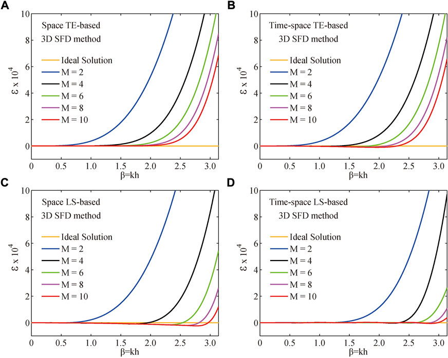
FIGURE 1. Variation curves of numerical dispersion ($\epsilon$) with the difference operator length ($M$) changing for the simple 3D homogeneous acoustic model (Model A). These subgraphs (A–D) indicate different 3D SFD methods listed in themselves.

FIGURE 2

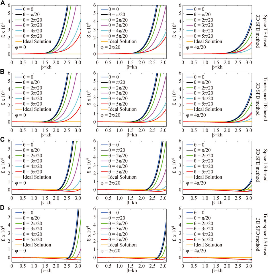
FIGURE 2. Variation curves of numerical dispersion ($\epsilon$) with the propagation angle ($\theta$) and azimuth angle ($\phi$) changing for the simple 3D homogeneous acoustic model (Model A). These subgraphs (A–D) indicate different 3D SFD methods listed in themselves.

Next, this above simple 3D homogeneous acoustic model (Model A) is again employed to analyze the algorithm stabilities of different 3D SFD methods. Figure 3 depicts the variation curves of stability factors ($\zeta$) of different 3D SFD methods for the simple 3D homogeneous acoustic model. From Figure 3, the stability of time-space domain TE-based 3D SFD method is better than that of space domain TE-based 3D SFD method and the difference between their stabilities is very small, the stability of space domain LS-based 3D SFD method is slightly worse compared with the previous two TE-based 3D SFD methods, and the stability of our optimized time-space domain LS-based 3D SFD method is worst, which suggests that our method has the strictest stability requirements at the same difference operator lengths ($M$) in these four 3D SFD methods mentioned in this paper. Moreover, the stability factors of these 3D SFD methods gradually decreases with the difference operator length increasing, which indicates that their stability conditions are gradually stricter with the difference operator length increasing. According to the stability conditions of different 3D SFD methods, this above conclusion means that the upper limit of courant number gradually decreases with the difference operator length increasing. For a given 3D model, under the condition of stable wavefield modeling, the increase of difference operator length means the decrease of courant number, and further means the decrease of time grid step or the increase of space grid step and these two changes are respectively adverse to reduce the computational cost and improve the modeling precision. For our optimized time-space domain LS-based 3D SFD method, the phenomenon is more serious thanks to its strictest stability condition, and therefore we need to pay more attention to coordinate the relationship among the difference operator length, space grid step and time grid step in its application.

FIGURE 3

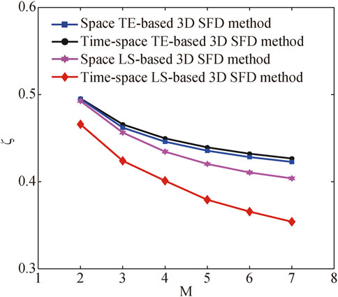
FIGURE 3. Variation curves of stability factors ($\zeta$) of different 3D SFD methods for the simple 3D homogeneous acoustic model (Model A).

Forward modeling examples

To further test and verify the superiority of our optimized time-space domain LS-based 3D SFD method, we use two models to compare and analyze the modeling precision of different 3D SFD methods, including a 3D homogenous acoustic model (Model B) and a complex 3D salt model. The model parameters of the former are: $x\times y\times z=4\mathrm{k}\mathrm{m}\times 4\mathrm{k}\mathrm{m}\times 4\mathrm{k}\mathrm{m}$, $v=3000\mathrm{m}/\mathrm{s}$, $\rho =2.0{\mathrm{g}/\mathrm{c}\mathrm{m}}^3$, $h=20\mathrm{m}$, and $\Delta t=1\mathrm{m}\mathrm{s}$, respectively. During the 3D wavefield modeling of this model, we define the source signal as the Ricker wavelet with $f_{center}=30\mathrm{H}\mathrm{z}$ and $T_{duration}=3\mathrm{s}$ which are respectively the central frequency and the total time of the seismic wavelet, and the source position is $\left(x,y,z\right)=\left(2\mathrm{k}\mathrm{m},2\mathrm{k}\mathrm{m},2\mathrm{k}\mathrm{m}\right)$. Figure 4 shows some 3D snapshots ($t=0.6\mathrm{s}$ and $t=1.4\mathrm{s}$) generated by different 3D SFD methods with different difference operator lengths ($M=3$ and $M=5$) for this 3D homogenous acoustic model. Figure 5 displays its corresponding 2D slices of these 3D snapshots shown in Figure 4 at different positions and different times. As can be seen from Figure 4, these four different 3D SFD methods can effectively simulate the propagation features of seismic wave in 3D acoustic model, but the simulation accuracy of different 3D SFD methods are different. According to Figures 4, 5, the snapshots of two TE-based 3D SFD methods contain obvious numerical dispersion indicated by these purple arrows which will seriously interfere with the useful seismic information when the difference operator length is equal to five ($M=5$). Although the space domain LS-based 3D SFD method can weaken this phenomenon to a certain extent, the numerical dispersion indicated by these purple arrows is still visible in its snapshots when the difference operator length is equal to five ($M=5$). When utilizing our optimized time-space domain LS-based 3D SFD method to modeling 3D seismic wavefields, the numerical dispersion indicated by these purple arrows is greatly suppressed and even almost invisible in its snapshots when the difference operator length is equal to three or five ($M=3$ or $M=5$), which suggests that our method can use a smaller difference operator length to effectively ensure higher simulation accuracy and reduce computing time compared with the other three conventional 3D SFD methods. In general, by comparing and analyzing the numerical dispersion of four different 3D SFD methods shown in Figures 4, 5, our optimized time-space domain LS-based 3D SFD method has the best modeling wavefields compared with the three conventional 3D SFD methods, because its snapshots do not contain obvious numerical dispersion indicated by these purple arrows and the waveforms in its snapshots are clearest. To compare the numerical dispersion of different 3D SFD methods more clearly, we draw the waveform curves of the 2D snapshots ($M=5$) shown in Figure 5 along different directions shown in Figure 6, and Figure 7 depicts these waveform curves. As can be seen from Figure 7, for the same 3D SFD method, the numerical dispersion in the vertical and horizontal directions (defined as Ⅰ and Ⅱ) is strong, while the numerical dispersion in the two diagonal directions (defined as Ⅲ and Ⅳ) is weak. When the wavefront passes, there are strong interference fluctuations in the snapshots for the two TE-based 3D SFD methods, these interference fluctuations are effectively weakened to a certain extent using the conventional space domain LS-based 3D SFD method, and our optimized time-space domain LS-based 3D SFD method can attenuate these interference fluctuations more effectively. Figure 8 shows the vibration curves simulated by different 3D SFD methods ($M=5$) for this 3D homogenous acoustic model at particle $\left(x,y,z\right)=\left(1.0\mathrm{k}\mathrm{m},1.0\mathrm{k}\mathrm{m},2.0\mathrm{k}\mathrm{m}\right)$. From Figure 8, the vibration amplitude of our optimized time-space domain LS-based 3D SFD method is the smallest after the wavefront passing through this particle in these four different 3D SFD methods, which further indicates that our optimized method can suppress numerical dispersion more effectively. One conclusion can be naturally generalized according to these analysis results: our optimized time-space domain LS-based 3D SFD method can obtain higher precision and higher quality 3D simulated wavefields than three conventional 3D SFD methods.

FIGURE 4

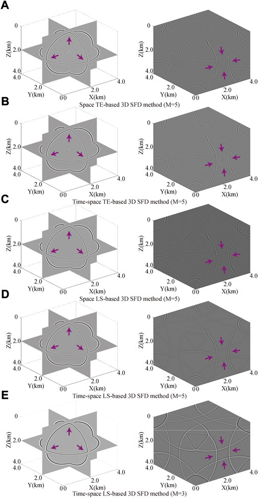
FIGURE 4. 3D snapshots at 0.6 and 1.4 s for the simple 3D homogeneous acoustic model (Model B). These subgraphs (A–E) indicate different 3D SFD methods with different difference operator lengths ($M=3$ and $M=5$) listed in themselves.

FIGURE 5

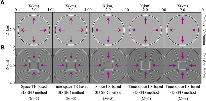
FIGURE 5. 2D slices of the 3D snapshots shown in Figure 4. The subgraphs (A,B) indicate different times, different positions and different 3D SFD methods with different difference operator lengths ($M=3$ and $M=5$) listed in themselves.

FIGURE 6

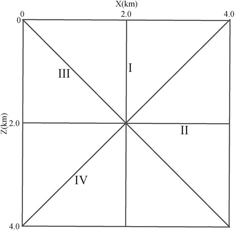
FIGURE 6. Different directions of waveform curves for the 2D slices shown in Figure 5.

FIGURE 7

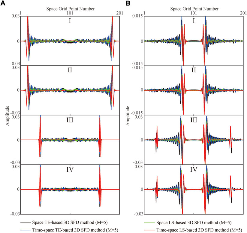
FIGURE 7. Waveform curves of the 2D snapshots ($M=5$) shown in Figure 5 for the simple 3D homogeneous acoustic model (Model B). (A) Waveform curves of the 2D snapshots at 0.6 s. (B) Waveform curves of the 2D snapshots at 1.4 s. I, II, III and IV represent the different directions shown in Figure 6.

FIGURE 8

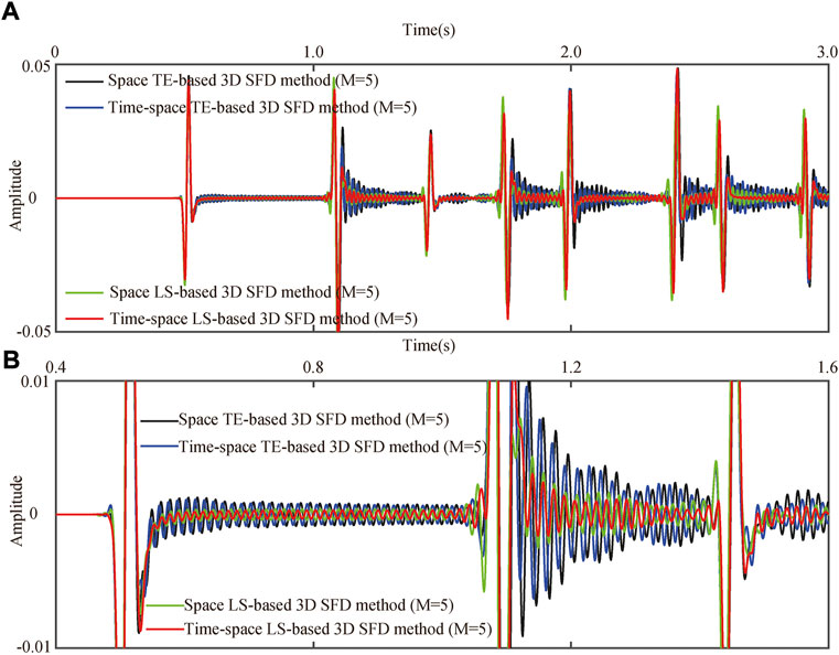
FIGURE 8. Vibration curves simulated by different 3D SFD methods ($M=5$) for the simple 3D homogeneous acoustic model (Model B) at particle $\left(x,y,z\right)=\left(1.0\mathrm{k}\mathrm{m},1.0\mathrm{k}\mathrm{m},2.0\mathrm{k}\mathrm{m}\right)$. (A) Full vibration curves. (B) Local magnification curves.

Figure 9 shows the velocity and density of the 3D SEG/EAGE salt model, and then we use it to test the applicability of our optimized time-space domain LS-based 3D SFD method for complex geological models. Other model parameters of this model are following: $x\times y\times z=6.76\mathrm{k}\mathrm{m}\times 6.76\mathrm{k}\mathrm{m}\times 4.2\mathrm{k}\mathrm{m}$, $h=20\mathrm{m}$, and $\Delta t=1\mathrm{m}\mathrm{s}$, respectively. For its 3D wavefield modeling, the source signal is the Ricker wavelet with $f_{center}=15\mathrm{H}\mathrm{z}$ and $T_{duration}=4\mathrm{s}$ which are respectively the central frequency and the total time of the seismic wavelet, and the source position is $\left(x,y,z\right)=\left(3.38\mathrm{k}\mathrm{m},3.38\mathrm{k}\mathrm{m},0\mathrm{k}\mathrm{m}\right)$. Figure 10 displays the 2D slices of the 3D snapshots ($t=1.6\mathrm{s}$) generated by different 3D SFD methods ($M=5$) at the different positions for this 3D SEG/EAGE salt model. According to Figure 10, we can find that these 3D SFD methods mentioned in this paper can effectively simulate the propagation characteristics of seismic wave in 3D complex geological models, but their numerical simulation accuracy are also different. From Figure 10, the obvious numerical dispersion indicated by these purple arrows exists in these snapshots of two TE-based 3D SFD methods, and this phenomenon is lightly weakened in these snapshots of conventional space domain LS-based 3D SFD method, but it is still visible indicated by these purple arrows. However, the numerical dispersion indicated by these purple arrows is best suppressed in these snapshots generated by our optimized time-space domain LS-based 3D SFD method. Figure 11 depicts the waveform curves of the 2D snapshots shown in Figure 10 and the positions of these waveform curves. From Figure 11, because the source wavelet is located on the surface of this model, there is obvious numerical dispersion in the shallow section of 3D snapshots for three conventional 3D SFD methods, and these numerical dispersion decreases with the depth increasing. Moreover, even in the shallow section, our optimized time-space domain LS-based 3D SFD method can suppress the numerical dispersion better compared with three conventional 3D SFD methods. Figure 12 and Figure 13 display the local 2D slices of the 3D seismic records generated by different 3D SFD methods ($M=5$) at the different positions along $x$ and $y$ directions for this 3D SEG/EAGE salt model, respectively. From Figure 12 and Figure 13, we can find that these synthetic seismograms of three conventional 3D SFD methods contain clearly visible numerical dispersion indicated by these purple arrows, which seriously interferes with the identification of direct waves and reflected waves. However, our optimized time-space domain LS-based 3D SFD method can more effectively suppress the numerical dispersion indicated by these purple arrows and obtain more accurate synthetic seismograms compared with the three conventional 3D SFD methods, which further proves that our optimized time-space domain LS-based 3D SFD method can improve the numerical simulation precision of 3D seismic wavefields more effectively.

FIGURE 9

FIGURE 9. 3D SEG/EAGE salt model. (A) Velocity. (B) Density.

FIGURE 10

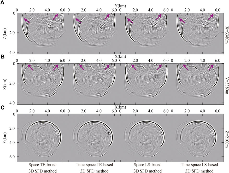
FIGURE 10. 2D slices of the 3D snapshots ($t=1.6\mathrm{s}$) generated by different 3D SFD methods ($M=5$) at the different positions for the 3D SEG/EAGE salt model. These subgraphs (A–C) indicate different positions and different 3D SFD methods listed in themselves.

FIGURE 11

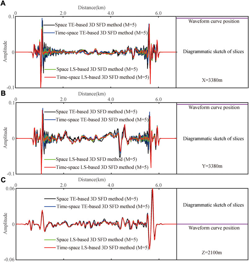
FIGURE 11. Waveform curves of the 2D snapshots ($M=5$) shown in Figure 10 and the positions of these waveform curves. (A) Waveform curves of the 2D snapshots at $x=3380\mathrm{m}$. (B) Waveform curves of the 2D snapshots at $y=3380\mathrm{m}$. (C) Waveform curves of the 2D snapshots at $z=2100\mathrm{m}$.

FIGURE 12

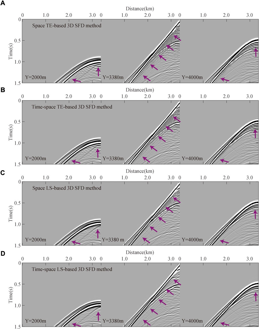
FIGURE 12. Local 2D slices of the 3D seismic records generated by different 3D SFD methods ($M=5$) along $x$ direction for the 3D SEG/EAGE salt model. These subgraphs (A–D) indicate different positions and different 3D SFD methods listed in themselves.

FIGURE 13

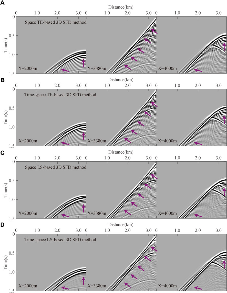
FIGURE 13. Local 2D slices of the 3D seismic records generated by different 3D SFD methods ($M=5$) along $y$ direction for the 3D SEG/EAGE salt model. These subgraphs (A–D) indicate different positions and different 3D SFD methods listed in themselves.

Discussion

In addition to the simulation accuracy and algorithm stability, the computational cost is also a significant evaluation index for 3D SFD methods. By analyzing these four different 3D SFD methods mentioned in the previous sections, we can find that the difference of their computational cost can be mainly reflected in the following two aspects: one is the computing time of SFD coefficients, the other is the computing time of 3D wavefield simulation. Because these four different 3D SFD methods all use Eq. 3 to calculate their corresponding 3D seismic wavefields at different times, there is a little difference between the computing time of their wavefield simulation process under the same conditions. We firstly discuss the difference between the computing time for their SFD coefficients. According to the calculation equations of different 3D SFD coefficients, the main factor affecting the corresponding computational cost is the difference operator length, especially for our optimized time-space domain LS-based 3D SFD method. Generally speaking, it will take a longer computing time with a larger difference operator length. Hence, we mainly compare and analyze the computational cost of different 3D SFD coefficients with different difference operator lengths under the same other conditions, and the results are listed in Table 1. According to Table 1, it takes little time to estimate their corresponding SFD coefficients for three conventional 3D SFD methods. In other words, the computational cost of their SFD coefficients can be negligible. Nevertheless, the computing time of SFD coefficients for our optimized time-space domain LS-based 3D SFD method is relatively long and it increases rapidly with the difference operator length increasing, because our optimized method needs to calculate a lot of triple integrals. To effectively reduce the application time of our optimized time-space domain LS-based 3D SFD method, we should first estimate its corresponding equivalent SFD coefficients and store them for a given 3D model, and then we can use these stored equivalent SFD coefficients to model the 3D seismic wavefields and even realize the 3D RTM.

TABLE 1

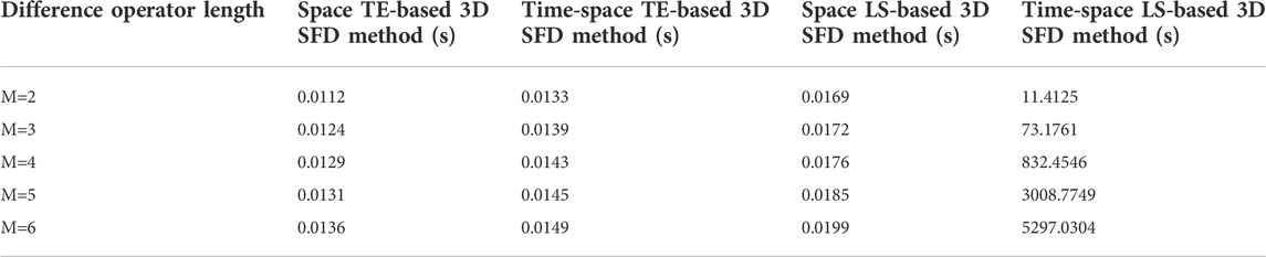
TABLE 1. Computational cost of four 3D SFD coefficients with different difference operator lengths.

To understand the computational cost of different 3D SFD methods more intuitively, we secondly compare the computing time of their wavefield simulation process for the 3D homogenous acoustic model (Model B), which is the sum of the computing time of wavefield simulation at different times. Figure 14 shows the computational cost of different 3D SFD methods with different difference operator lengths for this model B. As we can see in Figure 14, when the difference operator length is equal to five ($M=5$), the computing time of three conventional 3D SFD methods are almost the same for 3D wavefield simulation, and our optimized time-space domain LS-based 3D SFD method needs a slightly longer computing time compared with three conventional methods, but this time difference of wavefield simulation for our optimized method is tolerable. Combining with the previous forward modeling examples, when the difference operator length is equal to three ($M=3$), our optimized time-space domain LS-based 3D SFD method can not only simulate high precision 3D wavefields, but also greatly reduce the computing time of wavefield simulation compared with the other three conventional 3D SFD methods, which indicates that our optimized method can effectively save the computational cost of 3D wavefield simulation by reducing the difference operator length. According to the previous computational cost analysis, we should estimate and store the difference coefficients of our optimized time-space domain LS-based 3D SFD method in advance before wavefield modeling to effectively reduce the computing time of whole forward modeling for a given 3D model. This strategy can effectively reduce the difficulty of applying our optimized time-space domain LS-based 3D SFD method to 3D RTM, because it does not cause too much unnecessary time consumption during wavefield extrapolation.

FIGURE 14

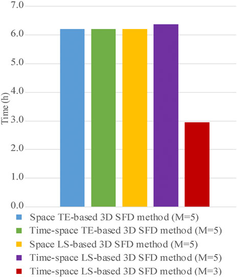
FIGURE 14. Computational cost of wavefield simulation of different 3D SFD methods with different difference operator lengths for the simple 3D homogeneous acoustic model (Model B).

Conclusion

A 3D numerical simulation is the core algorithm of 3D RTM, and its simulation accuracy affects the imaging accuracy of 3D RTM to a considerable degree. To achieve this goal effectively, we build on an optimized 3D SFD method using the time-space domain dispersion relation and the LS method to model the responses of seismic wave in 3D inhomogeneous model based on 2D seismic modeling case. Because this optimized time-space domain LS-based 3D SFD method makes full use of the advantages of the time-space domain dispersion equations and the LS method to estimate its corresponding SFD coefficients, it has weaker numerical dispersion and higher modeling precision theoretically than the conventional 3D SFD methods for 3D seismic wavefields. To compare and analyze the numerical dispersion, simulation accuracy, algorithm stability and computational cost for different 3D SFD methods, we use different 3D numerical models to test and verify the above four aspects. The numerical examples of different 3D models illustrate that our optimized time-space domain LS-based 3D SFD method can produce higher precision simulated 3D wavefields than three conventional 3D SFD methods. Moreover, the stability condition of our optimized time-space domain LS-based 3D SFD method becomes stricter than three conventional 3D SFD methods and it will progressively become worse when the difference operator length increases gradually. Finally, the computational cost of our optimized time-space domain LS-based 3D SFD method is also greater than that of three conventional 3D SFD methods, because it needs a long time to estimate its equivalent SFD coefficients and its wavefield modeling requires a slightly long computing time. However, our optimized time-space domain LS-based 3D SFD method can reduce the computational cost by reducing the difference operator length under the same modeling accuracy requirements.

Data availability statement

The raw data supporting the conclusions of this article will be made available by the authors, without undue reservation.

Author contributions

Conceptualization: WL and WW; methodology: WL, WW, and JY; code: WL and JY; writing–original draft: WL; writing–review and editing: WL, JY, and HW; funding acquisition: JC and JY.

Funding

This work is supported by the National Natural Science Foundation of China (Grant Nos. 42030812 and 42004103).

Acknowledgments

We are very grateful to Haihao Liu for his help in revising this English manuscript. We would also like to express thanks for the helpful comments and suggestions from the editors and reviewers.

Conflict of interest

The authors declare that the research was conducted in the absence of any commercial or financial relationships that could be construed as a potential conflict of interest.

Publisher’s note

All claims expressed in this article are solely those of the authors and do not necessarily represent those of their affiliated organizations, or those of the publisher, the editors and the reviewers. Any product that may be evaluated in this article, or claim that may be made by its manufacturer, is not guaranteed or endorsed by the publisher.

Supplementary material

The Supplementary Material for this article can be found online at: https://www.frontiersin.org/articles/10.3389/feart.2022.1004422/full#supplementary-material

References

Alkhalifah, T. (2013). Residual extrapolation operators for efficient wavefield construction. Geophys. J. Int. 193 (2), 1027–1034. doi:10.1093/gji/ggt040

CrossRef Full Text | Google Scholar

Bartolo, L. D., Do rs, S., and Mansur, W. J. (2012). A new family of finite-difference schemes to solve the heterogeneous acoustic wave equation. Geophysics 77 (5), T187–T199. doi:10.1190/geo2011-0345.1

CrossRef Full Text | Google Scholar

Cai, X. H., Liu, Y., Ren, Z. M., Wang, J. M., Chen, Z. D., Chen, K. Y., et al. (2015). Three-dimensional acoustic wave equation modeling based on the optimal finite-difference scheme. Appl. Geophys. 12 (3), 409–420. doi:10.1007/s11770-015-0496-y

CrossRef Full Text | Google Scholar

Dablain, M. A. (1986). The application of high-order differencing to the scalar wave equation. Geophysics 51 (1), 54–66. doi:10.1190/1.1442040

CrossRef Full Text | Google Scholar

Etgen, J. T., and O’Brien, M. J. (2007). Computational methods for large-scale 3D acoustic finite-difference modeling: A tutorial. Geophysics 72 (5), SM223–SM230. doi:10.1190/1.2753753

CrossRef Full Text | Google Scholar

Fan, N., Zhao, L. F., Xie, X. B., Tang, X. G., and Yao, Z. X. (2017). A general optimal method for a 2D frequency-domain finite-difference solution of scalar wave equation. Geophysics 82 (3), T121–T132. doi:10.1190/geo2016-0457.1

CrossRef Full Text | Google Scholar

Fornberg, B. (1987). The pseudospectral method: Comparisons with finite-differences for the elastic wave equation. Geophysics 52 (4), 483–501. doi:10.1190/1.1442319

CrossRef Full Text | Google Scholar

Graves, R. W. (1996). Simulating seismic wave propagation in 3D elastic media using staggered-grid finite-differences. Bull. Seismol. Soc. Am. 86 (4), 1091–1106. doi:10.1785/BSSA0860041091

CrossRef Full Text | Google Scholar

Huang, Q. H., Li, Z. H., and Wang, Y. B. (2010). A parallel 3D staggered grid pseudospectral time domain method for ground-penetrating radar wave simulation. J. Geophys. Res. 115 (B12), B12101–B12113. doi:10.1029/2010JB007711

CrossRef Full Text | Google Scholar

Liang, W. Q., Xu, X., Wang, Y. F., and Yang, C. C. (2018). A simplified staggered-grid finite-difference scheme and its linear solution for the first-order acoustic wave-equation modeling. J. Comput. Phys. 374 (1), 863–872. doi:10.1016/j.jcp.2018.08.011

CrossRef Full Text | Google Scholar

Liu, W., You, J. C., Cao, J. X., Liu, J. L., and Hu, R. Q. (2021). Variable density acoustic RTM of VSP data based on the time-space domain LS-based SFD method. Acta Geophys. 69, 1269–1285. doi:10.1007/s11600-021-00614-5

CrossRef Full Text | Google Scholar

Liu, Y. (2013). Globally optimal finite-difference schemes based on least squares. Geophysics 78 (4), T113–T132. doi:10.1190/geo2012-0480.1

CrossRef Full Text | Google Scholar

Liu, Y. (2014). Optimal staggered-grid finite-difference schemes based on least-squares for wave equation modelling. Geophys. J. Int. 197 (2), 1033–1047. doi:10.1093/gji/ggu032

CrossRef Full Text | Google Scholar

Liu, Y., and Sen, M. K. (2009a). A new time-space domain high-order finite-difference method for the acoustic wave equation. J. Comput. Phys. 228 (23), 8779–8806. doi:10.1016/j.jcp.2009.08.027

CrossRef Full Text | Google Scholar

Liu, Y., and Sen, M. K. (2009b). An implicit staggered-grid finite-difference method for seismic modelling. Geophys. J. Int. 179 (1), 459–474. doi:10.1111/j.1365-246X.2009.04305.x

CrossRef Full Text | Google Scholar

Liu, Y., and Sen, M. K. (2011a). Scalar wave equation modeling with time-space domain dispersion-relation-based staggered-grid finite-difference schemes. Bull. Seismol. Soc. Am. 101 (1), 141–159. doi:10.1785/0120100041

CrossRef Full Text | Google Scholar

Liu, Y., and Sen, M. K. (2011b). 3D acoustic wave modelling with time-space domain dispersion-relation-based finite-difference schemes and hybrid absorbing boundary conditions. Explor. Geophys. 42 (3), 176–189. doi:10.1071/EG11007

CrossRef Full Text | Google Scholar

Liu, Y., and Sen, M. K. (2013). Time-space domain dispersion-relation-based finite-difference method with arbitrary even-order accuracy for the 2D acoustic wave equation. J. Comput. Phys. 232, 327–345. doi:10.1016/j.jcp.2012.08.025

CrossRef Full Text | Google Scholar

Pitarka, A. (1999). 3D elastic finite-difference modeling of seismic motion using staggered grids with nonuniform spacing. Bull. Seismol. Soc. Am. 89 (1), 54–68. doi:10.1785/BSSA0890010054

CrossRef Full Text | Google Scholar

Ren, Z. M., and Li, Z. C. (2017). Temporal high-order staggered-grid finite-difference schemes for elastic wave propagation. Geophysics 82 (5), T207–T224. doi:10.1190/geo2017-0005.1

CrossRef Full Text | Google Scholar

Ren, Z. M., and Li, Z. C. (2019). High-order temporal and implicit spatial staggered-grid finite-difference operators for modelling seismic wave propagation. Geophys. J. Int. 217, 844–865. doi:10.1093/gji/ggz059

CrossRef Full Text | Google Scholar

Ren, Z. M., and Liu, Y. (2015). Acoustic and elastic modeling by optimal time-space-domain staggered-grid finite-difference schemes. Geophysics 80 (1), T17–T40. doi:10.1190/geo2014-0269.1

CrossRef Full Text | Google Scholar

Robertsson, J. O. A. (1996). A numerical free-surface condition for elastic/viscoelastic finite-difference modeling in the presence of topography. Geophysics 61 (6), 1921–1934. doi:10.1190/1.1444107

CrossRef Full Text | Google Scholar

Robertsson, J. O. A., Blanch, J. O., and Symes, W. W. (1994). Viscoelastic finite-difference modeling. Geophysics 59 (9), 1444–1456. doi:10.1190/1.1443701

CrossRef Full Text | Google Scholar

Shragge, J. (2014). Solving the 3D acoustic wave equation on generalized structured meshes: A finite-difference time-domain approach. Geophysics 79 (6), T363–T378. doi:10.1190/geo2014-0172.1

CrossRef Full Text | Google Scholar

Sotelo, E., Favino, M., and Gibson, R. L. (2021). Application of the generalized finite-element method to the acoustic wave simulation in exploration seismology. Geophysics 86 (1), T61–T74. doi:10.1190/geo2020-0324.1

CrossRef Full Text | Google Scholar

Teng, Y. C., and Dai, T. F. (1989). Finite-element prestack reverse-time migration for elastic waves. Geophysics 54 (9), 1204–1208. doi:10.1190/1.1442756

CrossRef Full Text | Google Scholar

Virieux, J. (1984). SH-wave propagation in heterogeneous media: Velocity-stress finite-difference method. Geophysics 49 (11), 1933–1942. doi:10.1190/1.1441605

CrossRef Full Text | Google Scholar

Virieux, J. (1986). P-SV wave propagation in heterogeneous media: Velocity-stress finite-difference method. Geophysics 51 (4), 889–901. doi:10.1190/1.1442147

CrossRef Full Text | Google Scholar

Wang, Y. F., Liang, W. Q., Nashed, Z., Li, X., Liang, G. H., and Yang, C. C. (2014). Seismic modeling by optimizing regularized staggered-grid finite-difference operators using a time-space-domain dispersion-relationship-preserving method. Geophysics 79 (5), T277–T285. doi:10.1190/geo2014-0078.1

CrossRef Full Text | Google Scholar

Wang, E. J., Carcione, J. M., Ba, J., Alajmi, M., and Qadrouh, A. N. (2019a). Nearly perfectly matched layer absorber for viscoelastic wave equations. Geophysics 84 (5), T335–T345. doi:10.1190/geo2018-0732.1

CrossRef Full Text | Google Scholar

Wang, E. J., Carcione, J. M., and Ba, J. (2019b). Wave simulation in double-porosity media based on the biot-Rayleigh theory. Geophysics 84 (4), WA11–WA21. doi:10.1190/GEO2018-0575.1

CrossRef Full Text | Google Scholar

Wang, E. J., Carcione, J. M., Cavallini, F., Botelho, M., and Ba, J. (2021). Generalized thermo-poroelasticity equations and wave simulation. Surv. Geophys. 42, 133–157. doi:10.1007/s10712-020-09619-z

CrossRef Full Text | Google Scholar

Wu, Z., and Alkhalifah, T. (2018). A highly accurate finite-difference method with minimum dispersion error for solving the Helmholtz equation. J. Comput. Phys. 365 (1), 350–361. doi:10.1016/j.jcp.2018.03.046

CrossRef Full Text | Google Scholar

Xu, S. G., and Liu, Y. (2018). Effective modeling and reverse-time migration for novel pure acoustic wave in arbitrary orthorhombic anisotropic media. J. Appl. Geophys. 150, 126–143. doi:10.1016/j.jappgeo.2018.01.013

CrossRef Full Text | Google Scholar

Xu, S. G., Liu, Y., Ren, Z. M., and Zhou, H. Y. (2019). Time-space-domain temporal high-order staggered-grid finite-difference schemes by combining orthogonality and pyramid stencils for 3D elastic-wave propagation. Geophysics 84 (4), T259–T282. doi:10.1190/geo2018-0551.1

CrossRef Full Text | Google Scholar

Yang, L., Yan, H. Y., and Liu, H. (2017). Optimal staggered-grid finite-difference schemes based on the minimax approximation method with the remez algorithm. Geophysics 82 (1), T27–T42. doi:10.1190/geo2016-0171.1

CrossRef Full Text | Google Scholar

Yomogida, K. J., and Etgen, T. (1993). 3-D wave propagation in the los angeles basin for the whittier-narrows earthquake. Bull. Seismol. Soc. Am. 83 (5), 1325–1344. doi:10.1785/BSSA0830051325

CrossRef Full Text | Google Scholar