Detecting Interdecadal Change in Western North Pacific Tropical Cyclone Genesis Based on Cluster Analysis Using pHash + Kmeans

Previous studies have noted an abrupt decrease in western North Pacific (WNP) tropical cyclone (TC) genesis frequency and a westward shift in genesis location since the late 1990s. The recent application of cluster analysis in TC research shows the effect of detecting the contribution of the Western North Pacific Subtropical High (WNPSH) and the interdecadal Pacific oscillation (IPO) on interdecadal change in WNP TCs. In this work, we also apply a clustering algorithm called pHash + Kmeans to group WNP TCs into three classes based on their genesis environmental conditions. The clustering results show that an abrupt decrease after 1998 is related primarily to a decrease in the dominant class (Class3, located mainly in the southern and eastern WNP), and an increase after 2010 occurs because of a new dominant class (Class1, located mainly in the northwestern WNP), which indicates that the WNP environment suppresses Class3 genesis after 1998 and enhances Class1 genesis after 2010. Three periods (P1: 1979–1997, P2: 1998–2010, and P3: 2011–2020) and three regions (SCS: 100°E-120°E, EQ-30°N; WNP1: 120°E-140°E, EQ-30°N; and WNP2: 140°E-160°W, EQ-30°N) are divided to further confirm the above findings. In P1, high (low) mid-level relative humidity (RH), intense (weak) low-level vorticity, and weak (strong) vertical wind shear (VWS) are distributed in WNP2 (SCS and WNP1), indicating suitable environmental conditions for TC genesis in WNP2 but unsuitable conditions in SCS and WNP1. This situation is the opposite in P2, leading to a decrease in genesis frequency and a westward shift in genesis location. In P3, strong low-pressure vorticity and thermodynamic conditions occur in SCS and WNP1, contributing to an increase in TC genesis frequency.

1 Introduction

In recent years, interdecadal variation in tropical cyclone (TC) activity over the western North Pacific (WNP) has been an area of active research. Numerous works have reported that a pronounced interdecadal change in WNP TC activity occurred in the late 1990s, including a decrease in genesis frequency and a westward shift in genesis location (Chan, 2008; Liu and Chan, 2008; Tu et al., 2011; Liu and Chan, 2013; Yokoi and Takayabu, 2013; He et al., 2015; Hong et al., 2016; Huangfu et al., 2017a; Huangfu et al., 2017b). These interdecadal changes are related to variations in environmental conditions and are influenced by large-scale circulations. Several studies (Tu et al., 2011; Liu and Chan, 2013; Zhao et al., 2014; Choi et al., 2015; Liu et al., 2019) have indicated that the inactive period of WNP TC activity is closely related to strengthening of vertical wind shear (VWS) over the eastern tropical WNP, which plays a vital role. Following these conclusions, Zhang et al. (2017) and Zhang et al. (2018) noted that the enhancement of warming over the North Atlantic also influences interdecadal change in WNP TC frequency by intensifying VWS in the southeastern WNP through the Walker circulation. Variation of sea surface temperature (SST) is also an essential influence on interdecadal change in WNP TCs (Kubota and Chan, 2009; Choi et al., 2015; He et al., 2015; Hsu et al., 2017; Wu R. et al., 2020). Hong et al. (2016) indicated that the La Niña–type pattern during the late 1990s is associated with an increase in VWS, anomalous vertical transport of water vapour, and increasing mid-level moisture, which is responsible for the shift in WNP TC genesis position. Hu et al. (2018) analysed the change in WNP TC genesis longitude and latitude separately and found that the change in mean longitude is closely linked to ENSO diversity, and the change in mean latitude is dominated by a warming WNP, which is induced by an interdecadal tendency of central Pacific La Niña–like events. Cao et al. (2020) indicated that a La Niña event and warming over the North Atlantic occurred in the 1990s and caused a northwestward shift in autumn TCs over the WNP. Additionally, the Western North Pacific Subtropical High (WNPSH) (Kim and Seo, 2016; Wu Q. et al., 2020), the East Asia winter monsoon (Choi et al., 2017), the monsoon trough (MT) (Huangfu et al., 2017a; Huangfu et al., 2017b), and the tropical upper tropospheric trough (Wu et al., 2015) are also essential in modulating interdecadal change in WNP TCs.

Some recent studies have attempted to understand TC activity in detail with the help of cluster analysis (e.g., Choi an Kim, 2009; Kim et al., 2011; Daloz et al., 2015; Kim and Seo, 2016; Boudreault et al., 2017; Ramsay et al., 2012, 2018). Clustering algorithms were applied to group TC cases into several classes based on their tracks. The TC cases in the different classes vary in position, intensity, and timing. Analysis of the contributors to the different classes enables a deeper, more detailed understanding of TC activity. A recent work by Zhao et al. (2018) grouped WNP TC tracks into three classes, of which the dominant class was closely related to the interdecadal Pacific oscillation (IPO). The relationship between the IPO and the dominant class was then analysed. The results show that the negative phase of the IPO during the late 1990s corresponds to a La Niña pattern, which intensified the Walker circulation and weakened the WNP MT, suppressing subsequent WNP TC genesis. Wu et al. (2020) also focused on one dominant class from clustering results and found modulation by interdecadal change of the WNPSH on the longitudinal shift of WNP TC tracks. These two works show that cluster analysis can potentially increase our understanding of interdecadal change in TC activity by analysing the dominant classes.

Regarding previous research, changing environmental conditions like SST and VWS play essential roles in the interdecadal change in WNP TC activity. In this case, we assume that the TC genesis environment can play the same role as TC tracks in clustering WNP TCs. Because of changes in environmental conditions, clustering results show distinct differences in time series. Different classes are concentrated in different periods, and analysing the dominant class in different periods helps indicate the interdecadal change in the WNP environment and WNP TC activity. According to previous works (e.g., Kim et al., 2011), clustering algorithms have limitations regarding TC tracks because the tracks have different shapes. However, selecting environmental fields of a fixed shape can avoid this problem. The properties and environmental conditions of each class are compared for further analysis of the interdecadal change in WNP TC genesis.

This paper is organized as follows: Section 2 introduces the datasets, clustering algorithm, and analysis methods. Section 3 contains the analysis of the clustering results. Section 4 further analyses the decadal change in TC genesis in the WNP based on the clustering results; the environmental conditions for the decadal change are also discussed. A summary and conclusion are provided in Section 5.

2 Data and Methods

2.1 Data

In this work, TC best-track data were obtained from the International Best Track Archive for Climate Stewardship (IBTrACS) dataset (Knapp et al., 2010; Knapp and Kruk, 2010), including the time, position, and intensity (maximum sustained wind speed, MSWS) of TCs at 6-h intervals. Here we used data during 1979–2020 to remove any questionable data from the pre-satellite era, and only TC cases of tropical depression intensity (MSWS>23 kts) were selected.

Several atmospheric and oceanic variables were used for clustering, including 6-hourly SST, 600 hPa relative humidity (RH), 850 hPa relative vorticity (RV), and wind at 850 and 200 hPa from the European Centre for Medium-Range Weather Forecasts (ECMWF) Reanalysis v5 (ERA5) hourly dataset (Hersbach et al., 2020). Wind data were used for calculating VWS between 850 and 200 hPa. For each TC case, we selected 9° × 9° environmental fields centred on the TC genesis position. The environmental fields consist of SST, RH, RV, and VWS with a spatial resolution of 1° × 1°, which refers to one sample as a 4 × 9 × 9 matrix. Accordingly, we built a dataset consisting of 1,081 TC genesis samples.

For further analysis of the interdecadal change in WNP TCs, monthly data for SST, 600 hPa RH, 850 hPa RV, specific humidity, and temperature at all profiles, wind at 850 hPa and 200 hPa, mean sea level pressure, and geopotential were also derived from the ERA5 monthly dataset.

2.2 Methods

2.2.1 PHash + Kmeans Clustering Algorithm

The clustering algorithm used in this study is the K-means clustering algorithm (Jain, 2010), one of the most widely used. It is an unsupervised machine learning algorithm, which means it can learn characteristics from data without external help. Its procedure is as follows: K centroids are randomly selected from the whole dataset to cluster data into different classes. The distance between each sample and the centroids is calculated for each sample in the dataset. Then based on the distance, different samples are allocated into the closest centroid, and k clusters are formed. In each cluster, a new centroid is then selected. This process is iterated to update the centroids and clusters until all centroids have little change.

In K-means, the distance is used to distinguish the similarity between samples and cluster centroids, by which the algorithm can group samples to the closest cluster. The classical K-means algorithm usually uses the Euclidian distance:

$distance= \frac{1}{n}\sqrt{{\displaystyle \sum }_{i=1}^n {(A_i-B_i)}^2}$

where n refers to the data count in one sample, and $A_i$ and $B_i$ refer to the $i$th data in samples A and B. The Euclidian distance focuses on the similarity of the value and ignores the global characteristics of the data. Therefore, although it has worked well in previous studies using clustered TC tracks, it is not suitable for the 3-dimensional environmental field data in our work. To prevent this, we propose the pHash + Kmeans algorithm, in which we select the perceptual hashing (pHash) value with the Hamming distance (Venkatesan et al., 2000) to replace the Euclidean distance.

The pHash algorithm derives the fingerprint of image data and is popular for distinguishing different images. Its procedure is as follows, for each matrix: 1) perform the discrete cosine transform (DCT) and get the DCT matrix; 2) calculate the mean value of the DCT matrix; and 3) calculate the pHash value: compare each data point in the DCT matrix with the mean value; greater than or equal to the mean value is recorded as 1, and less than the mean value is recorded as 0. The new matrix of 0 and 1 is called the pHash value. After getting the pHash value of each matrix, the Hamming distance (the Hamming distance between two matrices is the number of positions in which the values are different) of different matrices is calculated. The samples in our work are 4 × 9 × 9 matrices with four variables, so we first calculate the pHash value matrix of each variable, then concatenate all matrices into one to represent the pHash value of one sample. Figure 1 shows the detailed procedure of the pHash + Kmeans algorithm.

FIGURE 1

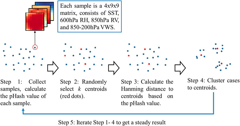
FIGURE 1. The procedure of the pHash + Kmeans algorithm.

The Dunn index (Dunn, 1973) and Separation index (Xie and Beni, 1991) are calculated to evaluate clustering results and determine the optimal cluster numbers. The Separation index is defined as the average distance between the cluster centroids, and the Dunn index refers to the ratio of the shortest distance between two samples from different clusters and the largest distance between two samples in the same cluster. For each number of classes, clustering is repeated five times and the average value of the indexes is calculated.

2.2.2 Analysis Methods

The number of TC genesis cases in each 2.5° × 2.5° grid over the WNP is counted. Spatial TC genesis frequency is defined as the average annual count for each grid. The position of TC genesis is defined as the first recorded position of each track in the IBTrACS dataset.

We also calculate the Genesis Potential Index (GPI) and the moist static energy (MSE) to help diagnose the variation in environmental conditions over the WNP. Emanuel and Nolan (2004) developed the GPI, defined as:

$GPI={\left|{10}^5\eta \right|}^{\frac{3}{2}}{\left(\frac{H}{50}\right)}^3{\left(\frac{V_{pot}}{70}\right)}^3{(1+0.1V_{shear})}^{-2}$

where $\eta$ is the absolute vorticity at 850 hPa, H is the relative humidity at 600 hPa in percent, $V_{pot}$ is the potential intensity, and $V_{shear}$ is the VWS magnitude between 850 and 200 hPa. The V_pot can be calculated based on the work of Bister and Emanuel (2002), as follows:

$V_{pot}^2=\frac{T_s}{T_o}\frac{C_k}{C_D}(CAP{E}^{\ast }-CAP{E}^b)$

where $T_s$ is SST, $T_o$ is the mean outflow temperature, $C_k$ is the exchange coefficient for enthalpy, $C_D$ is the drag coefficient, $CAP{E}^{\ast }$ is the convective available potential energy (CAPE) of air lifted from saturation at sea level in reference to the environmental sounding, and $CAP{E}^b$ is the CAPE of the boundary layer air.

MSE is defined as:

$MSE=C_{p}T+gz+L_{v}r$

where $g$ is the gravitational acceleration, $L_v$ is the latent heat of vaporisation, $C_p$ is the specific heat at constant pressure for air, T is the absolute temperature, z is the height above some reference level (either the local surface at z = 0 or the height where the ambient pressure is 100 kPa), and r is the water vapour mixing ratio in the air.

3 Analysis of Clustering Results and Detection of Interdecadal Change in WNP TC Genesis

The clustering results from the genesis environment will show different characteristics due to the close relationship between interdecadal change in WNP TCs and changes in the WNP environment. As the WNP environment changes, the dominant class will also change. Therefore, the clustering results will reflect the interdecadal change in TC genesis. Figure 2 gives the Dunn index and Separation index of the different class numbers. The Dunn index shows that the clustering results are steady, with more than two classes, and the Separation index indicates that clustering with three classes will achieve the best separation. Zhao et al. (2018) also indicated that some classes will share similar characteristics if the cluster number is too large and found that three clusters can have their own characteristics. Therefore, we clustered TCs into three classes named Class1, Class2, and Class3, with 256, 314, and 511 samples, respectively.

FIGURE 2

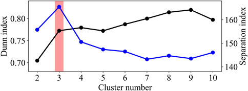
FIGURE 2. Evaluation indexes at each cluster number. The black line and dots refer to the Dunn index, and the blue line and dots refer to the Separation index. The red band refers to cluster number = 3, which has the optimal clustering effect.

Figures 3A–C shows the spatial genesis frequency. Class2 and Class3 are mainly in the southern and eastern WNP, while Class1 is farther north than Class2 and Class3, mainly in the northern South China Sea (SCS) and the northern Philippine Sea (PS). Figures 3D–F give the distribution of TC intensity of the three classes. Compared with Class1 and Class3, Class2 has more low-intensity cases, as its density peak is distributed at 50 kts. The white dot for the average value and the inner boxplot also indicate this. Class1 has an intensity distribution similar to that of Class2 but has more cases with intensity >100 kts. Class3 has an evenly distributed intensity, and its proportion of high-intensity cases is also higher than in Class1 or Class2, along with the highest average intensity.

FIGURE 3

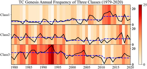
FIGURE 3. Time series of the TC genesis count in the three classes. The colour refers to the number of TC cases in the three classes each year. The x-axis refers to the year, the left y-axis refers to the class, and the right y-axis is the TC genesis count. The solid black lines refer to the time series of the TC genesis count in each class based on the IBTrACs dataset, and the dashed blue lines refer to the average value of TC genesis cases in P1, P2, and P3.

Figure 4 shows the time series of TC genesis counts in the three classes during 1979–2020. The heatmap gives the annual count of samples of each class, and the solid black lines present the time series of the three classes during 1979–2020. Class3 has a much higher proportion than the other classes in most years. After 1997, all three classes are inactive, and the most significant decrease occurs in Class3. This inactive period lasts until 2011, as Class1 increases and becomes the dominant class. The average value of the TC case count in 1979–1997, 1998–2010, and 2011–2020 is plotted as the blue dashed line, showing an increasing trend of Class1 and a decreasing trend of Class3. The sudden decrease of Class3 in 1998 corresponds to previous works showing that WNP TCs have been inactive since the late 1990s (e.g., Liu and Chan, 2013). According to Tang et al. (2020), a warming reacceleration trend has occurred in the northwestern WNP since 2011, possibly contributing to the increasing trend of Class1 during 2011–2020. These similarities show that the inactive period of WNP TCs after the late 1990s is possibly an inactive period of Class3, and the end of this inactive period after 2010 is related to the increase in Class1. Therefore, we infer that 1997 and 2010 are two important time nodes indicating interdecadal change in WNP TCs.

FIGURE 4

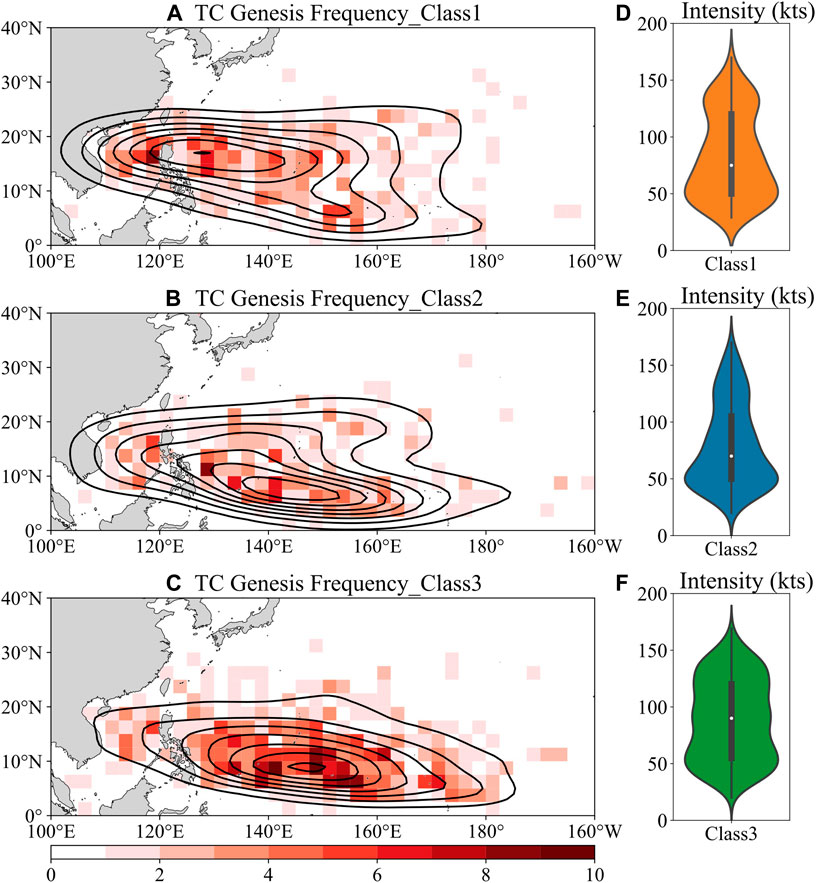
FIGURE 4. (A–C) are TC genesis frequency of the three classes, the contours are the KDE of genesis location, and the colour is the genesis frequency in one grid; (D–F) are the distribution of the intensity of each class. The colour and curve indicate the kernel density distribution for a given intensity. The thick inner line is the interquartile range, and the thin line is 95% of all cases. The white circle is the average of the intensity of each class.

In this work, the clustering results come mainly from the surrounding environmental fields of TC genesis. Therefore, the differences between classes result from variations in the WNP environment. Here we compare the composite fields of SST, RH, RV, and VWS of each class over the WNP in Figure 5. Suitable environmental conditions for TC genesis are highlighted by colours (SST >26°C and positive RV) and thick solid lines (RH > 60% and VWS <14 m s⁻¹). The figure shows that the genesis environments of Class2 and Class3 are similar, while that of Class1 shows apparent differences. For thermodynamic conditions, compared with Class2 and Class3, Class1 has a wider suitable area for TC genesis, including higher SST and RH, especially in SCS and PS. The area with suitable dynamic conditions in Class1 is farther north than in Class2 and Class3. The difference in RV is apparent west of 140°E, especially in SCS and PS. Combined with the intensity distribution in Figures 3E,F, we conclude that Class2 and Class3 share a similar WNP environment and have similar temporal and spatial distributions. Class2 contains mainly low-intensity cases with a lower proportion, and Class3 is mainly high-intensity cases with a dominant status.

FIGURE 5

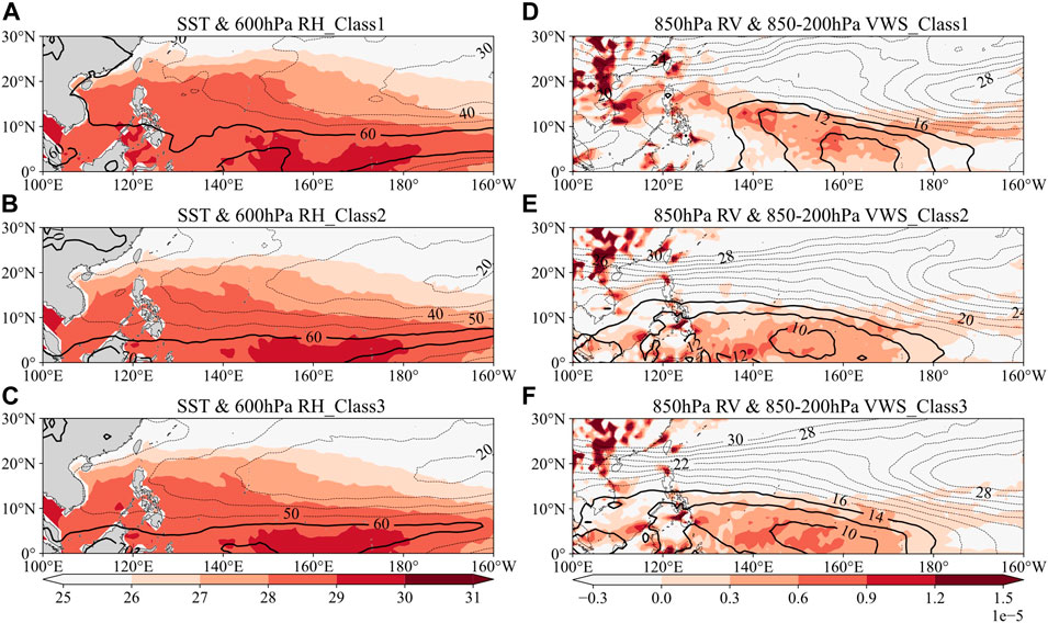
FIGURE 5. Composite environmental field of the three classes. (A–C) are the SST and 600 hPa RH. The solid thick lines refer to RH >= 60%, and the dashed thin line refers to RH < 60%. The colours refer to the SST, and only SST > 26°C is plotted; (D–F) are the 850 hPa RV and 850–200 hPa VWS. The solid thick lines refer to VWS <= 14, and the dashed thin line refers to VWS > 14. The colours refer to RV, and only positive RV is plotted.

WNP TC genesis cases can be clustered into three classes with different spatial and temporal characteristics based on environmental conditions. In different periods, the dominant class also changes. Before 1998, Class3 is the dominant class, but it substantially decreases after 1997. Then after the inactive period of all three classes in 1998–2010, Class1 becomes dominant after 2010. From Figures 3, 5, we find that the three classes have a noticeable difference in spatial distribution, which is related to the spatial distribution of environmental conditions. Class2 and Class3 may require a similar WNP environment, while the requirement of Class1 is different. Before 1998, the WNP environment is suitable for Class2 and Class3 but not for Class1. The southern and eastern WNP has more areas with suitable TC genesis conditions, thereby concentrating Class2 and Class3. We conclude that Class3 shows dominance during 1979–1997, but after 1997, a less suitable environment for Class2 and Class3 causes the abrupt decrease in Class2 and Class3, leading to the inactive period of the three classes during 1998–2010. Then after 2010, the WNP environment becomes more favourable for Class1, and the northwestward shift of the suitable areas for TC genesis causes more Class1 to form in the northwestern WNP. Still, the environment is not suitable for Class2 and Class3, so Class1 increases and becomes the dominant class. In conclusion, variations in the WNP environment lead to interdecadal change in WNP TC genesis, which is shown by the differences in the three classes in our clustering results.

To prove our assumption from the clustering results and further analyse the interdecadal change in WNP TC genesis, in the next section, we will separate the research periods into 1979–1997 (P1), 1998–2010 (P2), and 2011–2020 (P3) and then compare WNP TC genesis in each period. To distinguish the changes in different areas over the WNP, we will also divide the WNP into three regions based on longitude: SCS (100°E-120°E, EQ-30°N), WNP1(120°E-140°E, EQ-30°N), and WNP2 (140°E-160°W, EQ-30°N), and changes in the different regions will also be discussed.

4 Three Periods of Interdecadal Change in WNP TC Genesis and Their Differences

To confirm the variation in the WNP environment in the three periods, we first compare the environmental conditions over the WNP. The anomalies of SST, RH, RV, VWS, GPI, and MSE are shown in Figure 6. In P1, SST is negative in the WNP, except in southeastern WNP2, and RH also shows a similar distribution. The distribution of MSE also shows that the thermodynamic conditions are not favourable for TC genesis in SCS and WNP1. However, WNP2 has high positive RV and negative VWS, indicating suitable dynamic conditions. The WNP environment in P1 also shows similarities to the favourable environment of Class2 and Class3, as the suitable TC genesis conditions are concentrated mainly in WNP2. The environmental conditions in P2 are almost the opposite of those in P1 and become less favourable for Class2 and Class3. From P1 to P2, SST, RH, and MSE show an increase in SCS, WNP1, and northwestern WNP2 and a decrease in southeastern WNP2. Although the changes in RV and VWS are slight in SCS and WNP1, the high negative RV anomalies and positive VWS in WNP2 show that the dynamic conditions will suppress TC genesis in WNP2, which has also been reported in previous works (e.g., Zhang et al., 2017; Liu et al., 2019). GPI also shows that TCs are more likely to form in SCS and WNP1 than in WNP2. From P2 to P3, SST is still increasing and is positive at the basin scale. A slight decrease in RH occurs in SCS and WNP1, but RH is still positive in this area. The distribution of MSE also indicates a basin-wide strengthening of thermodynamic conditions from P2 to P3, similar to the Class1 genesis environment. Positive RV is distributed mainly in SCS and WNP1, much farther north and west than in P1 and P2, also showing similarities with Class1.

FIGURE 6

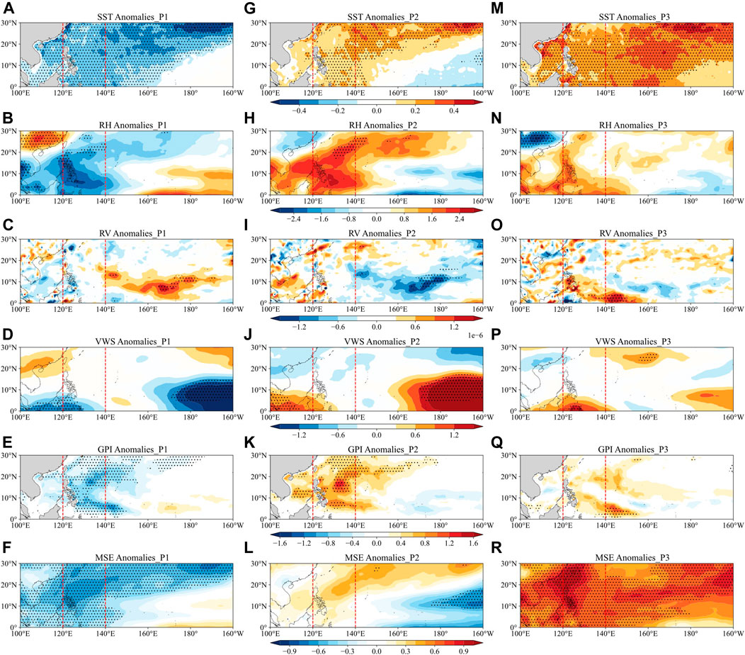
FIGURE 6. The anomalies of SST, 600 hPa RH, 850 hPa RV, 850–200 hPa VWS, GPI, and MSE. (A–F) are the environmental conditions in P1; (G–L) are the environmental conditions in P2; (M–R) are the environmental conditions in P3. The red dashed lines refer to longitude = 120°E and 140°E, which separate WNP into SCS, WNP1, and WNP2. The black dots are statistically significant at the 90% confidence level.

Given that the WNP environments in the three periods show apparent differences, we then further analyse the differences in WNP TCs in P1, P2, and P3, as shown in Figure 7. Figures 7A–C give the genesis frequency of each period. In P1, TCs form mainly in WNP2, and the highest KDE occurs around 150°E, 5°N, similar to Class2 and Class3. Figures 6A–F also show that in P1, WNP2 can provide a higher temperature, more mid-tropospheric moisture, stronger low-level vorticity, and weaker VWS than SCS and WNP1, indicating that more TCs can possibly form in WNP2 than in SCS or WNP1. From P1 to P2, the genesis frequency decreases in WNP2 but increases in SCS and WNP1. The KDE also shows a shift from WNP2 to WNP1, consistent with environmental conditions. From P2 to P3, TC genesis is still mainly in SCS and WNP1 but is more concentrated. The TC genesis frequency in each grid shows that more TCs form in SCS during P2-P3, mainly due to the enhancement of RV and SST. Figures 6G,M also show a warming trend over SCS, similar to the result of Tang et al. (2020). Figure 7D gives the temporal change of WNP TC genesis, showing an increasing trend in P1, but after the abrupt decrease in 1997, WNP TCs are inactive in P2, and then WNP TC genesis shows another increasing trend in P3. Figure 7E gives the time series of TC genesis counts in the three regions. In P1, TC counts in SCS and WNP1 remain at a low level, but TCs in WNP2 are active and show an increasing trend. After a sudden decrease in WNP2 and an increase in WNP1 in 1997, TC genesis becomes active in WNP1 and inactive in WNP2 during P2, and SCS is still inactive. The TC genesis frequency remains steady and shows little change in WNP1 and WNP2 from P2 to P3, but it remains an increasing trend in SCS in P3. In summary, the abrupt decrease in WNP TCs is a combination of a slight increase in WNP1 TCs and a substantial decrease in WNP2 TCs, which also leads to the inactive period in P2, and the increase in WNP TCs in P3 occurs mainly in SCS.

FIGURE 7

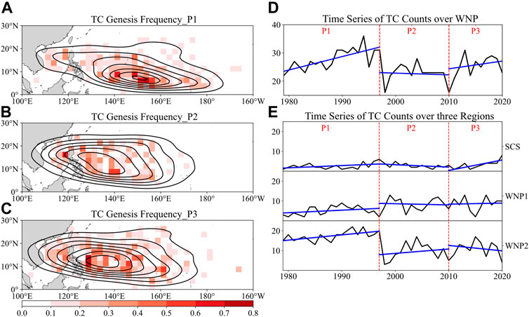
FIGURE 7. (A–C) are the TC genesis frequency in the three periods, the contours are the KDE of genesis location, and the colour is the genesis frequency in one grid; (D) is the time series of TC genesis counts during 1979–2020, the black line refers to the count from the IBTrACs dataset, and the blue lines are the trend lines of TC count change in P1, P2, and P3. The red dashed lines refer to 1997 and 2010 to separate P1, P2, and P3; (E) is similar to (D), but for the time series of TC genesis counts in SCS, WNP1, and WNP2.

5 Summary and Discussion

Interdecadal change in WNP TCs has been a hot research topic in recent years. Many works have discussed how WNP TC activity has changed in recent decades and the possible reasons. Previous studies have widely reported that an abrupt decrease in TC genesis and a northwestward shift in the TC-active region occurred around the late 1990s (e.g., Chan, 2008; Tu et al., 2011; Liu and Chan, 2013; He et al., 2015; Hong et al., 2016; Huangfu et al., 2017a; Huangfu et al., 2017b). Cluster analysis is used to group TC tracks into different classes and can potentially lead to increased understanding of WNP TC interdecadal change by analysing the relationship between the dominant class and possible contributors like the WNPSH and PDO (Zhao et al., 2018; Wu Q. et al., 2020). In this work, we built a pHash + Kmean algorithm in which the pHash value was used to represent the genesis environmental conditions of TCs. This algorithm was used to cluster WNP TCs during 1979–2020 into three classes: Class1, Class2, and Class3, with 256, 314, and 511 cases, respectively.

The clustering result shows that the dominant class varies in the different periods. Class3 has the highest proportion before 1998 and then has an abrupt decrease, while Class1 has a low count until 2010 and then becomes the dominant class. The composite WNP environment fields of the three classes also show differences: the environmental conditions of Class2 and Class3 are similar, with suitable genesis environmental conditions distributed in the southern and eastern WNP. In contrast, in the genesis environment for Class1, both high SST and RH have a broader distribution, and the area with positive RV and weak VWS also moves northward.

We found that the clustering results are closely related to changes in the WNP environment. The environmental conditions are more favourable for genesis in Class2 and Class3 during 1979–1997. The abrupt decrease in 1998 and the subsequent inactive period are caused by unfavourable environmental conditions for Class2 and Class3 genesis after 1997. After 2010, the WNP environment can lead to more Class1 genesis and less Class2 and Class3 genesis. To prove our assumption, we divided the study period into three periods (P1: 1979–1997, P2: 1998–2010, and P3: 2011–2020) and compared their differences. Additionally, as the three classes also show spatial differences, we divided the study region into three regions (SCS: 100°E-120°E, EQ-30°N; WNP1: 120°E-140°E, EQ-30°N; and WNP2: 140°E-180°W, EQ-30°N) for further analysis.

The environmental conditions in the three periods confirm our assumption that the clustering results come from changes in the WNP environment. In P1, positive (negative) RH anomalies and positive (negative) RV anomalies are distributed in WNP2 (SCS and WNP1), and positive VWS anomalies are distributed in WNP2, indicating that TC genesis is enhanced in WNP2 and suppressed in SCS and WNP1. This situation is similar to the genesis environment for Class2 and Class3, creating a concentration of TC genesis in the southeastern WNP. The WNP environment in P2 is the opposite of that in P1. The WNP2 environment suppresses TC genesis, while the SCS and WNP1 environments enhance TC genesis. This change causes the environment to be unsuitable for Class2 and Class3 genesis, leading to decreased WNP TC genesis frequency and a westward shift in genesis location. From P2 to P3, a strengthening of RV in SCS and WNP1 and basin-wide warming of SST in the WNP occurs, making the WNP environment more suitable for Class1 and leading to an increase in TC genesis frequency in P3.

Figure 7E shows that interdecadal change in WNP TCs in the late 1990s is indicated by a decrease over WNP2 and an increase over the eastern WNP. Changing dynamic conditions, especially the intensification of VWS over the southern and southeastern WNP, are demonstrated to be the significant modulator for the sudden decrease in eastern WNP TCs (Liu and Chan, 2013; Choi et al., 2015). As revealed by previous studies (Zhang et al., 2017; Zhang et al., 2018; Cao et al., 2020), this intensification of VWS is related to a shift in the Walker circulation induced by enhanced SST warming in the North Atlantic. In the late 1990s, the SST over the Pacific showed a La Niña–like mean state, which could also enhance VWS over the eastern WNP (Hsu et al., 2014; Choi et al., 2015; Hong et al., 2016; Hu et al., 2018; Liu et al., 2019; Cao et al., 2020). Huangfu et al. (2018) pointed out that the negative RV anomalies and positive VWS anomalies are possibly associated with downward motion anomalies over the central Pacific. The weakening and westward shift of the monsoon trough are also related factors in the weakening of RV (Choi et al., 2017; Hsu et al., 2017; Huangfu et al., 2017). According to Hong et al. (2016), the increase in TC frequency in the western WNP is controlled by strengthened thermodynamic conditions (e.g., warming SST and increased mid-level relative humidity), which are induced by the K-sharp warming over the Pacific.

Moreover, our clustering results indicate that 2011–2020 is a reactive period of WNP TCs, which is probably connected with SST warming over the northwestern WNP and the strengthening RV over the western WNP. As Tang et al. (2020) investigated, after 2010, a noticeable reacceleration of SST warming occurred in the northwestern WNP, especially offshore China. Zhang et al. (2019) also analysed the global annual mean surface temperature during 2014–2016, the recent warmest years on record, suggesting that global warming has accelerated since 2013. The variation trend of SST after 2010 may result in the interdecadal change in WNP TCs. We intend to examine the importance of different variables for the change in WNP TCs after 2010 and the physical mechanisms in follow-up research.

Data Availability Statement

We are grateful to the institutions providing data for this study. TC best-track data were provided by the International Best Track Archive for Climate Stewardship (IBTrACS, https://www.ncdc.noaa.gov/ibtracs/index.php?name=ib-v4-access). Atmospheric data were taken from the European Centre for Medium-Range Weather Forecasts Reanalysis v5 (ERA5, https://www.ecmwf.int/en/forecasts/datasets/reanalysis-datasets/era5).

Author Contributions

All authors listed have made a substantial, direct, and intellectual contribution to the work and approved it for publication.

Funding

This study is supported by the key project of National Natural Science Foundation of China (Grant 42192563 and Grant 42120104001), project of the Center for Ocean Research in Hong Kong and Macau (CORE), and the Hong Kong RGC General Research Fund (11300920).

Conflict of Interest

The authors declare that the research was conducted in the absence of any commercial or financial relationships that could be construed as a potential conflict of interest.

Publisher’s Note

All claims expressed in this article are solely those of the authors and do not necessarily represent those of their affiliated organizations, or those of the publisher, the editors, and the reviewers. Any product that may be evaluated in this article, or claim that may be made by its manufacturer, is not guaranteed or endorsed by the publisher.

References

Bister, M., and Emanuel, K. A. (2002). Low Frequency Variability of Tropical Cyclone Potential Intensity 1. Interannual to Interdecadal Variability. J. Geophys. Res. Atmospheres 107, D24. ACL 26-1-ACL 26-15. doi:10.1029/2001jd000776,

CrossRef Full Text | Google Scholar

Boudreault, M., Caron, L. P., and Camargo, S. J. (2017). Reanalysis of Climate Influences on Atlantic Tropical Cyclone Activity Using Cluster Analysis. J. Geophys. Res. Atmos. 122 (8), 4258–4280. doi:10.1002/2016jd026103

CrossRef Full Text | Google Scholar

Cao, X., Liu, Y., Wu, R., Bi, M., Dai, Y., and Cai, Z. (2020). Northwestwards Shift of Tropical Cyclone Genesis Position during Autumn over the Western North Pacific after the Late 1990s. Int. J. Climatol 40 (3), 1885–1899. doi:10.1002/joc.6310

CrossRef Full Text | Google Scholar

Chan, J. C. L. (2008). Decadal Variations of Intense Typhoon Occurrence in the Western North Pacific. Proc. R. Soc. A: Math. Phys. Eng. Sci. 464 (2089), 249–272. doi:10.1098/rspa.2007.0183

CrossRef Full Text | Google Scholar

Choi, J. W., Cha, Y., Kim, T., and Kim, H. D. (2017). Interdecadal Variation of Tropical Cyclone Genesis Frequency in Late Season over the Western North Pacific. Int. J. Climatol 37 (12), 4335–4346. doi:10.1002/joc.5090

CrossRef Full Text | Google Scholar

Choi, K.-S., Kim, B.-J., Choi, C.-Y., and Nam, J.-C. (2009). Cluster Analysis of Tropical Cyclones Making Landfall on the Korean Peninsula. Adv. Atmos. Sci. 26 (2), 202–210. doi:10.1007/s00376-009-0202-1

CrossRef Full Text | Google Scholar

Choi, Y., Ha, K.-Ja., Ho, C.-Hoi., and Chung, C. E. (2015). Interdecadal Change in Typhoon Genesis Condition over the Western North Pacific. Clim. Dyn. 45 (11), 3243–3255. doi:10.1007/s00382-015-2536-y

CrossRef Full Text | Google Scholar

Daloz, A. S., Camargo, S. J., Kossin, J. P., Emanuel, K., Horn, M., Jonas, J. A., et al. (2015). Cluster Analysis of Downscaled and Explicitly Simulated North Atlantic Tropical Cyclone Tracks. J. Clim. 28 (4), 1333–1361. doi:10.1175/jcli-d-13-00646.1

CrossRef Full Text | Google Scholar

Dunn, J. C. (1973). A Fuzzy Relative of the Isodata Process and its Use in Detecting Compact Well-Separated Clusters. J. Cybernetics 3, 32–57. doi:10.1080/01969727308546046

CrossRef Full Text | Google Scholar

Emanuel, K., and Nolan, D. S. (2004). “Tropical Cyclone Activity and the Global Climate System”.in 26th Conference on Hurricanes and Tropical Meteorology (Miami, FL, United States: American Meteorological Society), 240–241.

Google Scholar

He, H., Yang, J., Gong, D., Mao, R., Wang, Y., and Gao, M. (2015). Decadal Changes in Tropical Cyclone Activity over the Western North Pacific in the Late 1990s. Clim. Dyn. 45 (11), 3317–3329. doi:10.1007/s00382-015-2541-1

CrossRef Full Text | Google Scholar

Hersbach, H., Bell, B., Paul, B., Hirahara, S., Horányi, A., Muñoz‐Sabater, J., et al. (2020). The Era5 Global Reanalysis. Q. J. R. Meteorol. Soc. 146 (730), 1999–2049. doi:10.1002/qj.3803

CrossRef Full Text | Google Scholar

Hong, C.-C., Wu, Y.-K., and Li, T. (2016). Influence of Climate Regime Shift on the Interdecadal Change in Tropical Cyclone Activity over the Pacific Basin during the Middle to Late 1990s. Clim. Dyn. 47 (7), 2587–2600. doi:10.1007/s00382-016-2986-X

CrossRef Full Text | Google Scholar

Hsu, P.-C., Lee, T.-H., Tsou, C.-H., Chu, P.-S., Qian, Y., and Bi, M. (2017). Role of Scale Interactions in the Abrupt Change of Tropical Cyclone in Autumn over the Western North Pacific. Clim. Dyn. 49 (9), 3175–3192. doi:10.1007/s00382-016-3504-X

CrossRef Full Text | Google Scholar

Hsu, P.-C., Chu, P.-S., Murakami, H., and Zhao, X. (2014). An Abrupt Decrease in the Late-Season Typhoon Activity over the Western North Pacific*. J. Clim. 27 (11), 4296–4312. doi:10.1175/jcli-d-13-00417.1

CrossRef Full Text | Google Scholar

Hu, C., Zhang, C., Yang, S., Chen, D., and He, S. (2018). Perspective on the Northwestward Shift of Autumn Tropical Cyclogenesis Locations over the Western North Pacific from Shifting ENSO. Clim. Dyn. 51 (7), 2455–2465. doi:10.1007/s00382-017-4022-1

CrossRef Full Text | Google Scholar

Huangfu, J., Huang, R., and Chen, W. (2017a). Interdecadal Increase of Tropical Cyclone Genesis Frequency over the Western North Pacific in May. Int. J. Climatol. 37 (2), 1127–1130. doi:10.1002/joc.4760

CrossRef Full Text | Google Scholar

Huangfu, J., Huang, R., Chen, W., Feng, T., and Wu, L. (2017b). Interdecadal Variation of Tropical Cyclone Genesis and its Relationship to the Monsoon Trough over the Western North Pacific. Int. J. Climatol. 37 (9), 3587–3596. doi:10.1002/joc.4939

CrossRef Full Text | Google Scholar

Huangfu, J., Huang, R., and Chen, W. (2018). Interdecadal Variation of Tropical Cyclone Genesis and its Relationship to the Convective Activities over the Central Pacific. Clim. Dyn. 50 (3), 1439–1450. doi:10.1007/s00382-017-3697-7

CrossRef Full Text | Google Scholar

Jain, A. K. (2010). Data Clustering: 50 Years beyond K-Means. Pattern Recognition Lett. 31 (8), 651–666. doi:10.1016/j.patrec.2009.09.011

CrossRef Full Text | Google Scholar

Kim, H.-K., and Seo, K.-H. (2016). Cluster Analysis of Tropical Cyclone Tracks over the Western North Pacific Using a Self-Organizing Map. J. Clim. 29 (10), 3731–3751. doi:10.1175/jcli-d-15-0380.1

CrossRef Full Text | Google Scholar

Kim, H.-S., Kim, J.-H., Ho, C.-H., and Chu, P.-S. (2011). Pattern Classification of Typhoon Tracks Using the Fuzzy C-Means Clustering Method. J. Clim. 24 (2), 488–508. doi:10.1175/2010jcli3751.1

CrossRef Full Text | Google Scholar

Knapp, K. R., Kruk, M. C., Levinson, D. H., Diamond, H. J., and Neumann, C. J. (2010). The International Best Track Archive for Climate Stewardship (IBTrACS). Bull. Amer. Meteorol. Soc. 91 (3), 363–376. doi:10.1175/2009bams2755.1

CrossRef Full Text | Google Scholar

Knapp, K. R., and Kruk, M. C. (2010). Quantifying Interagency Differences in Tropical Cyclone Best-Track Wind Speed Estimates. Monthly Weather Rev. 138 (4), 1459–1473. doi:10.1175/2009mwr3123.1

CrossRef Full Text | Google Scholar

Kubota, H., and Chan, J. C. L. (2009). Interdecadal Variability of Tropical Cyclone Landfall in the Philippines from 1902 to 2005. Geophys. Res. Lett. 36 (12). doi:10.1029/2009gl038108

CrossRef Full Text | Google Scholar

Liu, C., Zhang, W., Geng, X., Stuecker, M. F., and Jin, F.-F. (2019). Modulation of Tropical Cyclones in the Southeastern Part of Western North Pacific by Tropical Pacific Decadal Variability. Clim. Dyn. 53 (7), 4475–4488. doi:10.1007/s00382-019-04799-w

CrossRef Full Text | Google Scholar

Liu, K. S., and Chan, J. C. (2008). "Interdecadal Variability of Western North Pacific Tropical Cyclone Tracks. J. Clim. 21 (17), 4464–4476. doi:10.1175/2008jcli2207.1

CrossRef Full Text | Google Scholar

Liu, K. S., and Chan, J. C. (2013). Inactive Period of Western North Pacific Tropical Cyclone Activity in 1998-2011. J. Clim. 26 (8), 2614–2630. doi:10.1175/jcli-d-12-00053.1

CrossRef Full Text | Google Scholar

Ramsay, H. A., Camargo, S. J., and Kim, D. (2012). Cluster Analysis of Tropical Cyclone Tracks in the Southern Hemisphere. Clim. Dyn. 39 (3-4), 897–917. doi:10.1007/s00382-011-1225-8

CrossRef Full Text | Google Scholar

Ramsay, H. A., Chand, S. S., and Camargo, S. J. (2018). A Statistical Assessment of Southern Hemisphere Tropical Cyclone Tracks in Climate Models. J. Clim. 31 (24), 10081–10104. doi:10.1175/jcli-d-18-0377.1

CrossRef Full Text | Google Scholar

Tang, Y., Huangfu, J., Huang, R., and Chen, W. (2020). Surface Warming Reacceleration in Offshore China and its Interdecadal Effects on the East Asia-Pacific Climate. Sci. Rep. 10 (1), 14811. doi:10.1038/s41598-020-71862-6

PubMed Abstract | CrossRef Full Text | Google Scholar

Tu, J.-Y., Chou, C., Huang, P., and Huang, R. (2011). An Abrupt Increase of Intense Typhoons over the Western North Pacific in Early Summer. Environ. Res. Lett. 6 (3), 034013. doi:10.1088/1748-9326/6/3/034013

CrossRef Full Text | Google Scholar

Venkatesan, R., Koon, S.-M., Jakubowski, M, H., and Moulin, P.(2000). “Robust Image Hashing”, in Paper presented at the Proceedings 2000 International Conference on Image Processing (Vancouver, BC, Canada, IEEE).

Google Scholar

Wu, L., Wang, C., and Wang, B. (2015). Westward Shift of Western North Pacific Tropical Cyclogenesis. Geophys. Res. Lett. 42 (5), 1537–1542. doi:10.1002/2015gl063450

CrossRef Full Text | Google Scholar

Wu, Q., Wang, X., and Tao, L. (2020). Interannual and Interdecadal Impact of Western North Pacific Subtropical High on Tropical Cyclone Activity. Clim. Dyn. 54 (3), 2237–2248. doi:10.1007/s00382-019-05110-7

CrossRef Full Text | Google Scholar

Wu, R., Cao, X., and Yang, Y. (2020). Interdecadal Change in the Relationship of the Western North Pacific Tropical Cyclogenesis Frequency to Tropical Indian and North Atlantic Ocean SST in Early 1990s. J. Geophys. Res. Atmospheres 125 (2), e2019JD031493. doi:10.1029/2019jd031493

CrossRef Full Text | Google Scholar

Xie, X. L., and Beni, G. (1991). A Validity Measure for Fuzzy Clustering. IEEE Trans. Pattern Anal. Machine Intell. 13 (8), 841–847. doi:10.1109/34.85677

CrossRef Full Text | Google Scholar

Yokoi, S., and Takayabu, Y. N. (2013). Attribution of Decadal Variability in Tropical Cyclone Passage Frequency over the Western North Pacific: A New Approach Emphasizing the Genesis Location of Cyclones. J. Clim. 26 (3), 973–987. doi:10.1175/jcli-d-12-00060.1

CrossRef Full Text | Google Scholar

Zhang, C., Li, S., Luo, F., and Huang, Z. (2019). The Global Warming Hiatus Has Faded Away: An Analysis of 2014-2016 Global Surface Air Temperatures. Int. J. Climatol 39 (12), 4853–4868. doi:10.1002/joc.6114

CrossRef Full Text | Google Scholar

Zhang, W., Vecchi, G. A., Villarini, G., Murakami, H., Rosati, A., Yang, X., et al. (2017). Modulation of Western North Pacific Tropical Cyclone Activity by the Atlantic Meridional Mode. Clim. Dyn. 48 (1-2), 631–647. doi:10.1007/s00382-016-3099-2

CrossRef Full Text | Google Scholar

Zhang, W., Vecchi, G. A., Murakami, H., Villarini, G., Delworth, T. L., Yang, X., et al. (2018). Dominant Role of Atlantic Multidecadal Oscillation in the Recent Decadal Changes in Western North Pacific Tropical Cyclone Activity. Geophys. Res. Lett. 45 (1), 354–362. doi:10.1002/2017gl076397

CrossRef Full Text | Google Scholar

Zhao, H., Chu, P.-S., Hsu, P.-C., and Murakami, H. (2014). Exploratory Analysis of Extremely Low Tropical Cyclone Activity during the Late-Season of 2010 and 1998 over the Western North Pacific and the South China Sea. J. Adv. Model. Earth Syst. 6 (4), 1141–1153. doi:10.1002/2014ms000381

CrossRef Full Text | Google Scholar

Zhao, J., Zhan, R., Wang, Y., and Xu, H. (2018). Contribution of the Interdecadal Pacific Oscillation to the Recent Abrupt Decrease in Tropical Cyclone Genesis Frequency over the Western North Pacific since 1998. J. Clim. 31 (20), 8211–8224. doi:10.1175/jcli-d-18-0202.1

CrossRef Full Text | Google Scholar