Correlations of Rock-Physics Model Parameters From Bayesian Analysis: Pressure- and Porosity-Dependent Models Applied to Unconsolidated Sands

Correlations of rock-physics model inputs are important to know to help design informative prior models within integrated reservoir-characterization workflows. A Bayesian framework is optimal to determine such correlations. Within that framework, we use velocity and porosity measurements on unconsolidated, dry, and clean sands. Three pressure- and three porosity-dependent rock-physics models are applied to the data to examine relationships among the inputs. As with any Bayesian formulation, we define a prior model and calculate the likelihood in order to evaluate the posterior. With relatively few inputs to consider for each rock-physics model, we found that sampling the posterior exhaustively to be convenient. The results of the Bayesian analyses are multivariate histograms that indicate most likely values of the input parameters given the data to which the rock-physics model was fit. When the Bayesian procedure is repeated many times for the same data, but with different prior models, correlations emerged among the input parameters in a rock-physics model. These correlations were not known previously. Implications, for the pressure- and porosity-dependent models examined here, are that these correlations should be utilized when applying these models to other relevant data sets. Furthermore, additional rock-physics models should be examined similarly to determine any potential correlations in their inputs. These correlations can then be taken advantage of in forward and inverse problems posed in reservoir characterization.

Introduction

Correlations of input parameters in a rock-physics model is always of concern, particularly when a model contains multiple inputs. Analysis of those correlations, however, is often performed in trial-and-error fashion when visually fitting a model to data. In doing so, any quantitative links among the input parameters could be overlooked inadvertently. The purpose of this work is to identify significant correlations among model parameters. This process is done for established rock-physics models. Three are pressure-dependent models, and three are porosity-dependent models, each used in conjunction with well characterized and controlled laboratory data. The model parameters are tested within a Bayesian framework where the models drawn from the posterior are used to identify most likely parameters or combinations of parameters when quantitatively fitting the models to data. This aspect is important within the context of reservoir characterization, and the analyses demonstrated here would allow us to define informative prior distributions within relevant workflows.

Many examples consist of a Bayesian formulation or framework to estimate rock properties and/or facies from seismic or other geophysical data. A short list includes Buland and Omre (2003); Spikes et al. (2007); Bosch et al. (2010); Rimstad et al. (2012); Ray et al. (2013); Kemper and Gunning (2014); Jullum and Kolbjørnsen (2016); de Figueiredo et al. (2017); Grana et al. (2017); de Figueiredo et al. (2018); Grana (2018); de Figueiredo et al. (2019); Grana (2020); and Nawaz et al. (2020). In all these efforts, the end goal is to obtain an estimate and the associated uncertainty of some facies and/or rock-property distributions from subsurface data. Moreover, these efforts must address disparate spatial scales and measurement types that must be reconciled to provide the estimate and associated uncertainty of subsurface rock properties (e.g., Ba et al., 2013; Pang et al., 2019; and ; Pang et al., 2021). These methods include the explicit use of a rock-physics model within the formulation or not (e.g., Avseth et al., 2005; Mavko et al., 2020); and Grana et al., 2021). The work we present here is different and unique because it directly examines the fit of rock-physics models to controlled laboratory data with the intention to determine correlations among the input parameters. Prior and posterior models are the underpinning of the approach, but the related information regarding linkages among the parameters is the primary emphasis. The results suggest which model might be easier or better to use than the others in a qualitative sense. Importantly, the results include previously unknown correlations for the three pressure-dependent and three porosity-dependent rock-physics models under consideration. This work is by no means exhaustive in terms of the examination of multiple models or data sets. The results for the rock-physics models studied here should be used with other relevant data. Furthermore, the method should be applied to other models and appropriate data to determine correlations among their inputs.

Conventional inversion techniques based on local optimization methods are prone to being trapped in local minima of the objective function closest to the starting model. In those techniques, uncertainty is estimated using the covariance matrix computed at the optimal (local) model. First, this approach gives incorrect estimates when the optimization becomes trapped in one of the local minima. Second, even if the optimization can find the globally optimal solution, covariance-based uncertainty estimates would be incorrect in that the uncertainties would be underestimated (e.g., Sen and Stoffa, 1996). The approach taken here is a sampling approach in which we carry out exhaustive sampling. Therefore, our approach is not prone to becoming trapped in local minima.

Materials and Methods

Data

We use the published data set from Zimmer (2003) and Zimmer et al. (2007a); Zimmer et al. (2007b), comprised of clean, dry, unconsolidated sands. Laboratory measurements consisted of compressional-and shear-wave velocities and porosity as a function of pressure for 15 different samples. Eight of those samples were reconstituted sands, named Gulf of Mexico, Pomponio, Santa Cruz Dry 1, Santa Cruz Dry 2, Sa Big Dry, SA Small Dry, Galveston Bay, and Merritt. Figure 1A is a plot of all those data sets of P-wave velocity ($V_P$) as a function of pressure (P). The velocity of each sample increases with increasing pressure, but at a different rate. Of the eight samples, we selected two, the Galveston Bay (black points in Figure 1B) and Merritt samples (gray points), to demonstrate the pressure-dependent version of this method. The reason to choose these two data sets is that they represent two distinct $V_P$-P trends. Figure 1B contains data from those two samples plus models reproduced from Zimmer et al. (2007a).

FIGURE 1

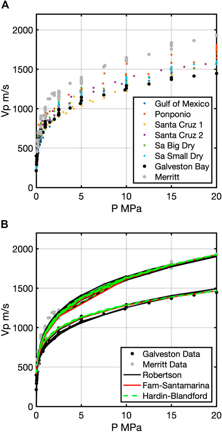
FIGURE 1. (A) Plot of P-wave velocity as a function of pressure for all the reconsolidated sand samples. The two used in the study here are the Galveston Bay data (black points) and the Merritt data (gray) points. In (B) the Galveston Bay and Merritt are replotted and overlain on them are the Robertson model (solid black line), Fam-Santamarina (red), and Hardin-Blandford (green). All three have a similar qualitative fit to the two data sets.

For the porosity-dependent models, we use all data from all reconstituted sands and glass beads. Figure 2A shows the compressional modulus ($M$) as a function of porosity ($\varphi$) for all 15 samples. The glass beads were of various sizes and size distributions (GB stands for glass beads). The terms Big, Small, and Tiny refer to sizes of the glass beads, GB35 stands for 35% Tiny mixed with larger bead sizes, and Broad means a wide range of bead sizes. Figure 2B is the same data as in Figure 2A except the color code is the log₁₀ of pressure. Last in Figure 2C, all the data are plotted in gray. For the Bayesian and sensitivity analysis, we select a subset of the data. That subset of data used for each rock-physics model was slightly different (red, green, and blue). In addition, we select two different subsets that represent different pressures (lower red, green, and blue points versus the upper ones). We refer to the lower set as data set 1 and the upper as data set 2.

FIGURE 2

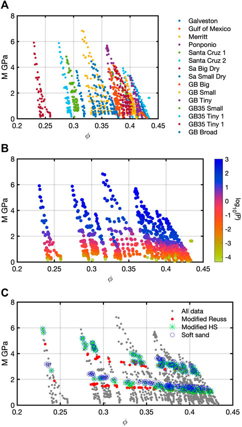
FIGURE 2. (A) Measured data (compressional modulus M) as a function of porosity color-coded by sample name. Sa refers to Santa Cruz, and GB refers to glass bead followed by the size. (B) The same data as in a) except color-coded by the log₁₀(P) for all 15 samples. For the rock-physics models used in the Bayesian analysis, slightly different subsets of the data are necessary to select. An initial model is visually fit, and then data within a 3% of that model are selected to use with that particular model (modified Reuss, modified Hashin-Strikman, and soft sand). We use two subsets (C) that correspond to different pressures and the different models.

Models

Pressure-Dependent Models

Two models are used to represent $V_P$ as a function $P$ for dry measurements (Zimmer et al., 2007a). The Robertson et al. (1995) model (R) is

$V_P=(A-Be){\left(\frac{P}{p_a}\right)}^{n/2}.(1)$

In Equation 1, $P$ is the measured effective pressure (equal to confining pressure for the dry samples), $p_a$ is the atmospheric pressure, $e=\varphi /(1-\varphi )$, the void ratio, where $\varphi$ is the measured porosity. The fitting parameters are $A$, $B$, and $n$.

The Fam and Santamarina (1997) Model is

$V_P=OC{R}^{k}S{\left(\frac{P}{p_a}\right)}^{n/2}.(2)$

For this model, the pressures are defined as the same as in Eq. 1. The $OCR$ term is the over-consolidation ratio, defined as $OCR=\max \left(P\right)/P$. Fitting parameters are $S$ and the two exponents $k$ and $n$.

The Hardin and Blandford (1989) model (HB) in Eq. 3,

$M=OC{R}^{k}S{p}_a^{1-n}{P}^n,(3)$

is a function of elastic moduli rather than velocity. These moduli could be the bulk, shear, or compressional moduli. The terms of pressure and $OCR$ are defined as in Eq. 2. The fitting parameters are $S$, $k$, and $n$.

Porosity-Dependent Models

Three rock-physics models were used in the Bayesian analysis. The first two were published in Zimmer et al. (2007b). Those two models are the modified Reuss

$\frac{1}{M}=\frac{f_{df}}{M_{df}}+\frac{f_{\text{Qtz}}}{M_{\text{Qtz}}}(4)$

and modified Hashin-Strikman (HS) models

$K^{\text{HS}}=K_{df}+\frac{f_{\text{Qtz}}}{{\left(K_{\text{Qtz}}-K_{df}\right)}^{-1}+f_{df}{\left(K_{df}+\frac{4}{3}{\mu }_{df}\right)}^{-1}}(5)$

${\mu }^{\text{HS}}={\mu }_{df}+\frac{f_{\text{Qtz}}}{{\left({\mu }_{\text{Qtz}}-{\mu }_{df}\right)}^{-1}+\frac{2f_{df}\left(K_{df}+2{\mu }_{df}\right)}{5{\mu }_{df}\left(K_{df}+\frac{4}{3}{\mu }_{df}\right)}}(6)$

In Equation 4, $M$ is the effective elastic modulus (bulk, shear, or compressional), $M_{df}$ is the dry frame elastic modulus (measured) at the current pressure, and $M_{\text{Qtz}}$ is the elastic modulus of quartz mineral. The fraction of the dry frame modulus is $f_{df}=\varphi /{\varphi }_0$. The ${\varphi }_0$ term is the porosity specifically from the current pressure but from the highest porosity sample, which is the Santa Cruz Dry 2 sample (Figure 2A). Last is the quartz mineral fraction, $f_{\text{Qtz}}=1-f_{df}$. Two parameters ($M_{df} and {\varphi }_0$) are the fitting parameters that are varied in the Bayesian analysis. These two parameters are measured as well, but single values of them correspond to one individual model. Therefore, the measured values are treated as mean values with uncertainty around them.

Equations 5, 6 are $K^{\text{HS}}$ and ${\mu }^{\text{HS}}$, the effective bulk and shear moduli, respectively, and the equations contain terms equivalent to those in Eq. 1 except for bulk and shear moduli instead of compressional modulus. Three terms are the fitting parameters for this model ($K_{df}$, ${\mu }_{df}$, and ${\varphi }_0$).

The third model used for porosity and pressure is the soft-sand model (Dvorkin and Nur, 1996), which was not used in the Zimmer et al. (2007b) paper. We introduce it here to demonstrate the effects of additional input parameters, beyond the number in the modified Reuss and Hashin-Strikman models. The soft-sand model combines Hertz-Mindlin (Mindlin, 1949) contact theory with modified Hashin-Strikman formulations to represent unconsolidated sands. The Hertz-Mindlin theory expresses the effective bulk and shear moduli, $K_{\text{HM}}$ and ${\mu }_{\text{HM}}$, respectively, for a dry random pack of identical spherical grains at a hydrostatic pressure, $P$.

$K_{\text{HM}}={\left[\frac{C_n^2{(1-{\varphi }_c)}^2{\mu }^2}{18{\pi }^2{\left(1-\nu \right)}^2}P\right]}^{\frac{1}{3}}(7)$

${\mu }_{\text{HM}}=\frac{5-4\nu }{5\left(2-\nu \right)}{\left[\frac{3C_n^2{(1-{\varphi }_c)}^2{\mu }^2}{2{\pi }^2{\left(1-\nu \right)}^2}P\right]}^{\frac{1}{3}}(8)$

Included in these equations are the mineral shear modulus and Poisson’s ratio ($\mu$ and $\nu$), the coordination number or average number of grain-to-grain contacts ($C_n$), and the critical porosity (${\varphi }_c$), the porosity at which a shear modulus can be sustained. These equations for the soft-sand model are used to formulate a type of dry rock, modified Hashin-Strikman lower bound for porosities from zero to ${\varphi }_c$ and separate calculations at ${\varphi }_c$ for the effective elastic moduli. In the calculations at ${\varphi }_c$, an additional term arises called the shear stiffness reduction ($SSR$), which compensates for no friction in the spherical grain pack. Refer to Dvorkin and Nur (1996) for these details. The fitting parameters for the soft-sand model are the P, ${\varphi }_c$, $C_n$, and $SSR$.

Bayesian Analysis

We reproduced a subset of the models published in Zimmer et al. (2007a). We used the Galveston Bay sand sample and fit Eqs 1–3 using the published values for the fitting parameters (Table 1). Then we applied Bayesian analysis to determine which inputs into the rock physics model have correlations among them. This approach includes a quantitative match of model to data. More specifically (i.e., Ulrych et al., 2001; Tarantola, 2005; Sen, 2006; Sen and Stoffa, 2013) we compute the likelihood (l(d|m)) with a given prior (p(m)), whose product is proportional to the posterior probability distribution ($\sigma \left(m|d\right)$) or PPD in Eq. 9

$\sigma \left(\mathbf{m}|\mathbf{d}\right)\propto l\left(\mathbf{d}|\mathbf{m}\right)p\left(\mathbf{m}\right),(9)$

Where d is the data vector, and m is the model. The likelihood function is

$l\left(\mathbf{d}|\mathbf{m}\right)\propto \exp \left(-E\left(\mathbf{m}\right)\right),(10)$

Where

$E\left(\mathbf{m}\right)={\left(\mathbf{d}-g\left(\mathbf{m}\right)\right)}^T{\mathbf{C}}_D^{-1}\left(\mathbf{d}-g\left(\mathbf{m}\right)\right),(11)$

TABLE 1

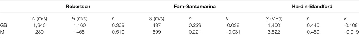
TABLE 1. Published values (Zimmer et al., 2007a) of the model parameters for the three pressure-dependent models for the Galveston Bay sample (GB) and the Merritt sample (M).

In Equation 11, g(m) is the forward modeling operator on the model, and C_D is the data covariance matrix (assuming Gaussian noise). The operator g(m) is a rock physics model in this case, where the inputs into that model are contained in m as a vector. The data-model comparison in Eq. 11 is equivalent to a least-squares fit of the model to the data. Equation 12 is the Gaussian prior where m_prior is the prior model mean, and C_M is the prior model covariance matrix.

$p\left(\mathbf{m}\right)\propto exp \left[{\left(\mathbf{m}-{\mathbf{m}}_{prior}\right)}^T{\mathbf{C}}_M^{-1}\left(\mathbf{m}-{\mathbf{m}}_{prior}\right)\right](12)$

The number of model parameters (three) is small for each of the models. Therefore, we find it convenient to sample exhaustively from the PPD rather than Monte Carlo Markov chain sampling. In other words, we draw many samples from the prior and evaluate the PPD for each model using Eq. 9. None of the rock-physics models are linear. Accordingly, the likelihood function becomes non-Gaussian, so an analytical solution for the posterior cannot be computed.

For the pressure-dependent problem, a trivariate Gaussian random distribution is used as the prior pdf. However, a sufficient number of models must be drawn, but the time to run a sufficient number of models must be considered. The number N = 300 was determined via trial and error to be sufficient that did not require significant computation time, and this size was used for the three rock-physics models. In addition to the size of the model, the prior mean model and covariance matrix are user defined. The means were set to the values in Table 1. The covariance matrices, however, had to be tested and determined via trial and error. This process was necessary to ensure that the collection of computed rock-physics models fell reasonably close to the data and without significant scatter among them. The posterior is a trivariate histogram of size 300 × 300 × 300. That size comes from calculating a model for every combination of inputs. We analyze bivariate joint histograms of the prior model and posterior, so any pair of values must be considered together rather than one conditional upon the other.

The number of model parameters for the porosity-dependent rock-physics models is two, three, and four, where each is a relatively small number. We again sampled exhaustively the PPD. The prior model is a multivariate Gaussian random distribution for each rock-physics model. Via trial and error, the number 2 × 2000 was determined sufficient for the modified Reuss model, where the 2 is number of inputs, and 2000 is the length of the prior model. For the modified HS model, the size 3 × 750 was deemed sufficient. Last, for the soft-sand model, 4 × 125 was found to be a sufficient number. Because of the exhaustive sampling, the size of the posterior for the modified Reuss is 2000 × 2000; 750 × 750 × 750 for the modified HS, and 125 × 125 × 125 × 125 for the soft-sand model. For analysis of the results, we examine bivariate joint histograms computed from the posterior alongside bivariates of the prior model.

For the porosity-dependent models, the user most also define the mean of the prior model and its covariance matrix. Table 2 contains the mean values. For the modified Reuss model, the two values come from the highest porosity sample at that pressure, which is the $\varphi$ and M from the Santa Cruz Dry 2 sample. The same type of values provided for the mean for the modified HS model, where the three values were $\varphi$, K, and $\mu$ from the Santa Cruz Dry 2 sample. Last, the mean for the soft-sand model contained the pressure value from the Santa Cruz Dry 2 sample, and the ${\varphi }_c$, $C_n$, and $SSR$ values were set to the values based on the initial model (Table 2). The covariance matrices in each case were determined using trial and error to ensure that the set of forward rock-physics models were relatively close to the data and with minimal scatter among the models.

TABLE 2

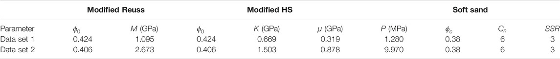
TABLE 2. Mean values for the multivariate random Gaussian prior models for data set 1 and data 2 for the three porosity-dependent rock-physics models.

Starting Models and Data Selection

For the porosity-dependent models, the selected data in Figure 2C had to be chosen for each of the three rock-physics models. If the data were too far away from the forward models, the objective function becomes large, and the likelihood and posterior values become very small. To select the data, a starting model was computed using the mean values in Table 2. Then data were selected based on 3% around the starting model. The data covariance (C_D ) was estimated assuming 5% error in the data. The starting models are displayed in relevant subsequent figures. Table 3 contains the number of selected data points for data sets 1 and 2 for the three rock-physics models.

TABLE 3

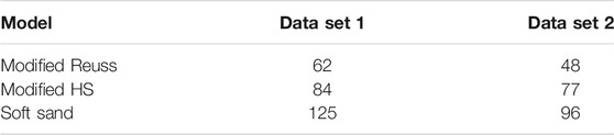
TABLE 3. Number of data points selected for each data set and for each rock-physics model.

Results

Pressure-Dependent Models

As aforementioned, the first step is to reproduce the models from Zimmer et al. (2007a). Figure 1B shows the fit of Eqs 1–3 to the Galveston Bay (black points) and Merritt (gray points) data. The solid black lines are the R model fits to the Galveston Bay and Merritt data. Red and green dashed lines are the FS and HB models, respectively, fit to the two data sets. Table 1 contains the fitting coefficients from Zimmer et al. (2007a) for the three models.

We applied the Bayesian formulation for the three models to the Galveston Bay data. The length of the Galveston Bay data vector was 58x1, and C_D was estimated assuming 5% error in the data, which is typical of in these types of laboratory measurements. For the R model, the three dimensions of the trivariate normal random distribution corresponded to A, B, and n. First, m was generated, where the means for the three variables are the A, B, and n values in Table 1 and a covariance matrix with diagonal [50 (m/s) 50 (m/s) 0.0002]. Off-diagonal terms were zero. The size of m was 3x300, so 300³ models were evaluated.

Figures 3A,B contain the prior model and posterior bivariate histograms, respectively, for A-B. Figures 3C,D correspond to the bivariate histograms for variables A-n, and 3E and 3F to B-n. In all the bivariate histograms for the prior model, one peak is apparent that is close to the mean. These histograms for the prior model are Gaussian although they might not always appear to be because the full trivariate has been marginalized in one direction. The posterior histogram for A-B shows a clear unimodal distribution peaking at a point different from the prior model mean. The posterior for A-n or B-n, however, is broad over A (or B) but shows a narrow range for n. When these posterior histogram for A and B is displayed in a logarithmic plot, it appears Gaussian, but the linear plot much more clearly identifies the highest peak. For the other two posterior histograms on a logarithmic plot, more than one value of n corresponds to broad ranges of A or B. Again, the linear plot by far indicates the n value with the highest frequency.

FIGURE 3

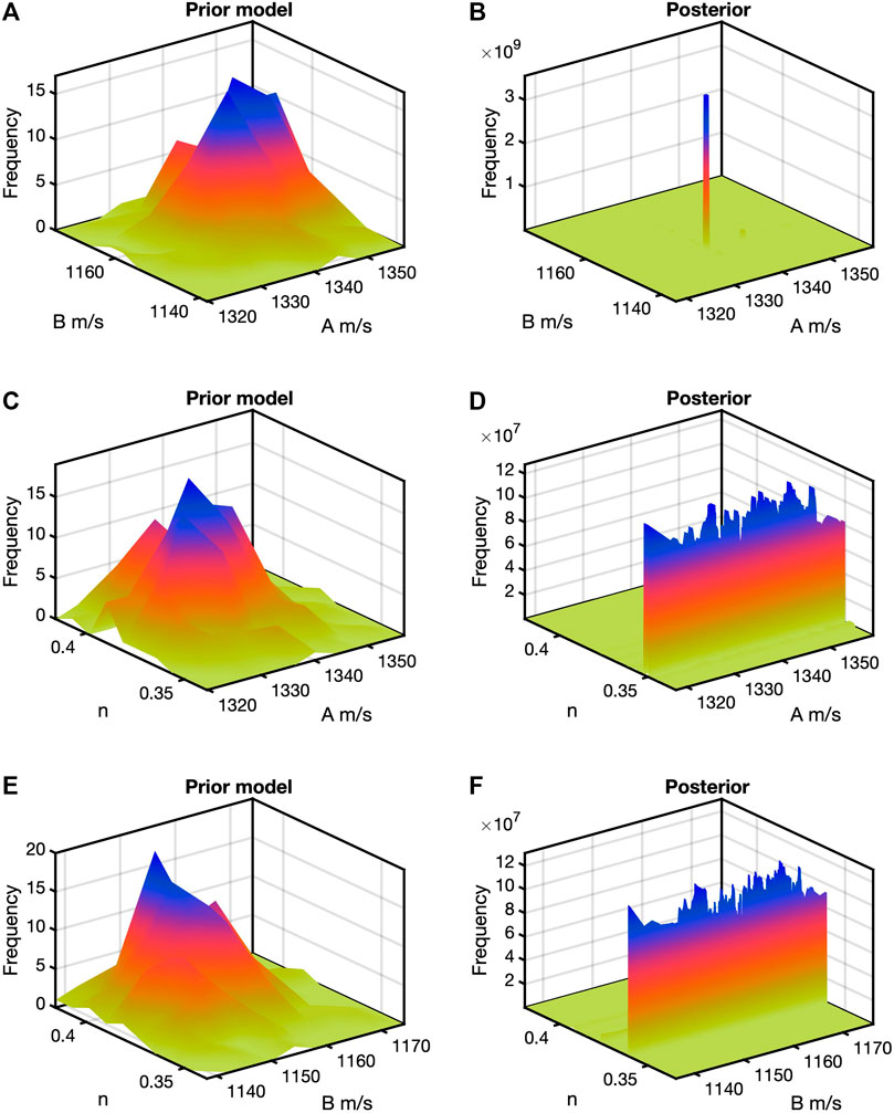
FIGURE 3. Bayesian analysis results for the Robertson model. In (A,B) are the bivariate prior model histogram and posterior histogram, respectively, for the joint A-B pair. The peak of the prior model histogram is at the mean, but the isolated peak in the posterior does not fall at the mean. The model and posterior bivariate distributions for the A-n pair are in (C,D), respectively. The prior model is a normal distribution by design, but the posterior indicates a very narrow range for n with and wide range of A values. The B-n pairs in (E,F) resemble those in (C,D).

The same procedure used with the R model was repeated using the FS and HB models. For both, the size of m was 3x300, and the means for m are in Table 1 for S, n, and k. The diagonal of the covariance matrix for m in the FS model was [43.7 (m/s) 0.0005 0.0011]. For the HB model, the covariance diagonal for m was [145 (MPa) 0.0004 0.0032].

Figure 4 shows the results for the FS model where the layout is the same as Figure 3 except for the different variables. Figures 4A,B are the prior model and posterior for the S-n pair, respectively, 4C and 4D for S-n, and 4E and 4F for n-k. Of the three posterior histograms, the S-n pair shows one clear peak, and the other two show a narrow for k with wider ranges for S or n. Bivariate histogram results for the HB model are in Figure 5. The prior model bivariate histogram for the S-n pair is in Figure 5A and the posterior in Figure 5B. The posterior shows a narrow range for n and a wide range of S (Figure 5B). In Figure 5C (the S-k pair), the central peak is at the mean value, and the corresponding posterior (Figure 5D) shows an isolated S-k pair with high frequency away from the prior model mean. The histogram in Figure 5F shows a narrow range of n for a wide range of k.

FIGURE 4

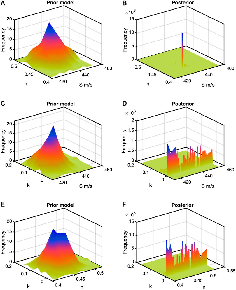
FIGURE 4. Bivariate histograms for the Fam-Santamarina model. (A,B) correspond to the S-n, pair, (C,D) to S-k, and (E,F) to n-k. The posterior histogram for S-n (B) shows an isolated high-frequency peak away from the mean in (A). In the other two posterior plots, a narrow range of k shows large frequencies for a wide range of S (E) and n (F).

FIGURE 5

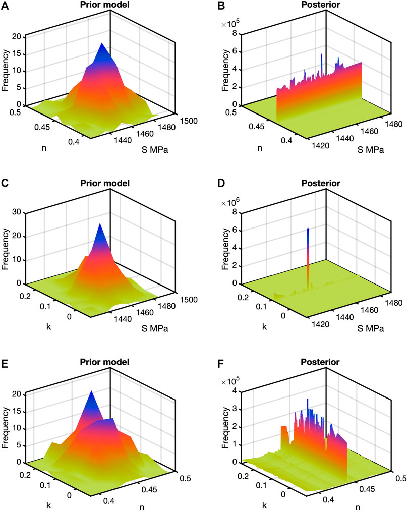
FIGURE 5. Model and posterior histograms for the Hardin-Blandford results. The juxtaposition is the same as in Figure 5. Different from the Fam-Santamarina model, the posterior in (A) shows a narrow range of n and wide range of S. The posterior in (D) shows an isolated peak for the S-k pair. Last the posterior in (F) show a narrow range of n for a wide range of k.

Next, we ran the three rock physics models for 100 trials with the Galveston Bay data where m was different for each trial. The mean and covariance matrices for each m remained the same, but the values in the random trivariate normal distribution differed from trial to trial. In all cases, the model size was 3x300. For each trial for the R model, the A-B pair corresponding to the highest frequency was selected using the information in the A-B posterior histogram in Figure 3B. To obtain n, the A-n posterior histogram maximum value was used (Figure 3D). Figure 6A exhibits these results, which indicate correlation among the three variables. Figure 6B displays the data, a selection of prior models (blue), and in gray the 100 maximum a posterior (MAP) results from the R model computed from the points in Figure 6A. The number of prior models is a small fraction of 1% of the number of computed models. Figures 6C,D show the corresponding plots for the FS model. The highest-frequency inputs for Figure 6C came from Figure 4B for S and n and 5F for k. Figures 6E,F show the same type of results for the HB model. Inputs for Figure 6E came from the values of S and k in Figure 5D and n from Figure 5F. Of the three, the MAP models in Figure 6B overall cluster more closely to the data than do the models in Figures 6D,F.

FIGURE 6

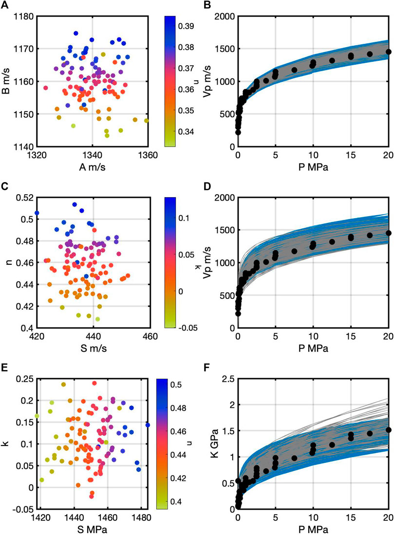
FIGURE 6. (A) Most likely values of A and B color coded by n for 100 trials of the Robertson model on the Galveston data. Correlation is evident among the three parameters. (B) contains the Galveston Bay data (points), a selection of prior models (gray), and MAP models (gray) from the 100 trials for each most likely value of A, B, and n from (A). The plots in (C) contains most likely values for the Fam-Santamarina model; in (D) are a selection of prior models (blue), and the 100 MAP models (gray). Last, the corresponding plots for the Hardin-Blandford model are in (E,F).

We then applied the Bayesian formulation for the three pressure-dependent rock-physics models to the Merritt data (Figure 1). The length of the Merritt data vector was 112 × 1, and C_D was estimated based on 5% data error. For the R model, the means for the three variables are the A, B, and n values in Table 1 and a covariance matrix with diagonal [50 (m/s) 50 (m/s) 0.0008]. Off-diagonal terms were zero. The size of m was 3 × 300, so 3003 models were evaluated. The means for m are in Table 1 for S, n, and k for the FS and HB models. The diagonal of the covariance matrix for m in the FS model was [59.9 (m/s) 0.0009 0.0001]. For the HB model, the covariance diagonal for m was [352 (MPa) 2x10⁻⁶ 9.6⁻⁸].

Results for the three rock-physics models applied to the Merritt data resemble those from the Galveston Bay data. Posterior bivariate histograms show overall similar features except for different values for the inputs. For the sake of the space, individual prior and posterior histograms are not displayed. Figure 7 contains plots akin to those in Figure 6 where most likely data pairs are selected for each model from the 100 trials; the corresponding MAP models and selections of prior models are also plotted with the Merritt data. Correlations among the R model inputs are similar for the Merritt (Figure 7A) and Galveston (Figure 6A) data. The MAP models in Figure 7B come from those points in Figure 7A. The corresponding plots from the FS model are in Figures 7C,D; for the HB model, the plots are Figures 7E,F.

FIGURE 7

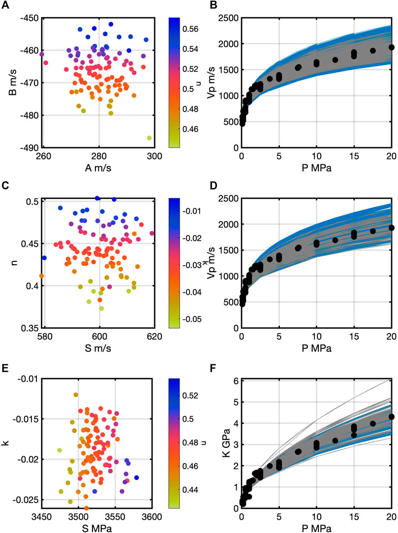
FIGURE 7. (A) Scatter plot of most likely values of A and B color coded by n for 100 trials of the Robertson model on the Merritt data. Correlation among the three parameters is present much like Figure 6A. In (B) are the Merritt data, a selection of prior models (blue), and the MAP models (gray) from the 100 trials for each most likely value of A, B, and n. In (C,D) are corresponding plots for the Fam-Santamarina model and the Hardin-Blandford model in (E,F).

Porosity-Dependent Models

We applied the Bayesian analysis first for the modified Reuss model to data set 1 (Figure 2C). The mean of m is in Table 2 along with a covariance matrix with diagonal [3.818x10⁻⁴ 0.010 (GPa)]. Off-diagonal terms were zero. Table 3 shows the number of data points. Figure 8A is the prior model bivariate histogram, and Figure 8B is the corresponding posterior bivariate histogram for the modified Reuss model applied to data set 1. The prior histogram is a random 2D Gaussian, and the posterior shows a narrow range of ${\varphi }_0$ for a wide range of $M_{df}$. The z-axis is displayed on a linear scale. If displayed on a logarithmic scale, other pairs of values have non-zero frequencies. but the plot on the linear scale much more clearly identifies the highest frequency value of ${\varphi }_0$.

FIGURE 8

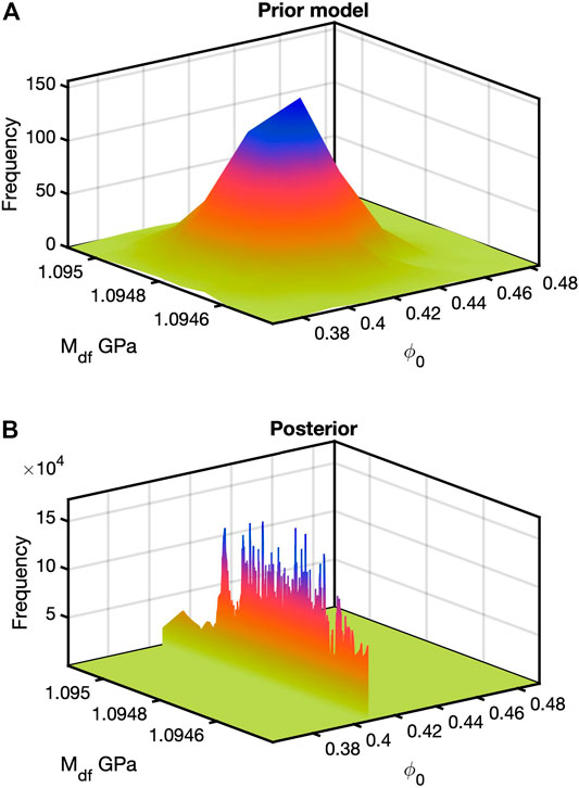
FIGURE 8. Bivariate histograms for the prior model (A) and posterior (B) for data set 1 and the modified Reuss model. In this case, the prior model and posterior are two dimensional. The joint bivariate in b) contains a very narrow range of ${\varphi }_0$ for a wide range of $M_{df}$. Other values have a non-zero frequency but with much lower values than the high-frequency visible range.

Next for data set 1, the Bayesian analysis was run using the modified HS model. Table 2 contains the mean of m. The diagonal of the covariance matrix was [2.121 × 10⁻⁴ 0.017 (GPa) 0.008 (GPa)] with off-diagonal terms set to zero. Figure 9 contains six bivariate histograms, for three prior models and three posteriors. With the number of input terms at three, the prior model and the full posterior are trivariate. Thus, we marginalize the prior and posterior in one direction to obtain the bivariates for display. Figures 9A,B are the prior model and posterior, respectfully, for ${\varphi }_0$-$K_{df}$. The prior is Gaussian, and the posterior shows a narrow, isolated value of ${\varphi }_0$ for a range of $K_{df}$. In Figures 9C,D, the bivariate histograms correspond to ${\varphi }_0$-${\mu }_{df}$; Figures 9E,F contain the bivariates for the pair of $K_{df}$ and ${\mu }_{df}$. Figure 9D is similar to Figure 9B with a narrow range of ${\varphi }_0$ for a range of ${\mu }_{df}$. Last the bivariate histogram in Figure 9F shows a high-frequency combination of $K_{df}$ and ${\mu }_{df}$.

FIGURE 9

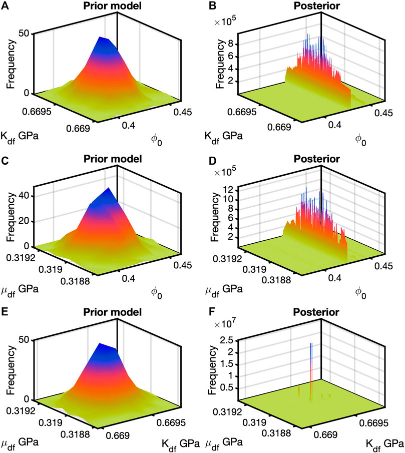
FIGURE 9. Example results from the modified HS model applied to data set 1. Bivariates for ${\varphi }_0$- $K_{df}$ pairs are in (A,B), ${\varphi }_0$-${\mu }_{df}$ in (C,D), and $K_{df}$-${\mu }_{df}$ in (E) and (F). A high-frequency peak is present in the posterior in (F). The other two posteriors show a very narrow range for ${\varphi }_0$ but wide ranges of ${\mu }_{df}$ and $K_{df}$.

The third porosity-dependent model applied to data set 1 was the soft-sand model. The diagonal of the covariance matrix was [0.006 (MPa) 0.002 0.030 0.015] with off-diagonal terms set to zero. Table 2 contains the mean values for the four variables. Figure 10 exhibits 12 bivariate histograms, half prior models and half posteriors. This number comes from computing each pair from the 4D full posterior. Figures 10A–C are prior model histograms for the pairs of P with ${\varphi }_c$, $C_n$, and $SSR$, respectively. Beneath those in Figures 10D–F are their corresponding posteriors. The posterior in Figure 10D shows a narrow range of ${\varphi }_c$ for a wide range of P. In Figures 10E,F, high-frequency pairs of P-$C_n$ and P-$SSR$ are present, respectively. Prior model bivariates for ${\varphi }_c$-$C_n$, ${\varphi }_c$-$SSR$, and $C_n$-$SSR$ are in Figures 10G–I and the corresponding posteriors in Figures 10J–L. The two posteriors of ${\varphi }_c$-$C_n$ and ${\varphi }_c$-$SSR$ show narrow ranges of one term and a broad range of the other. The posterior in Figure 10L indicates a high-frequency pair of $C_n$ and $SSR$.

FIGURE 10

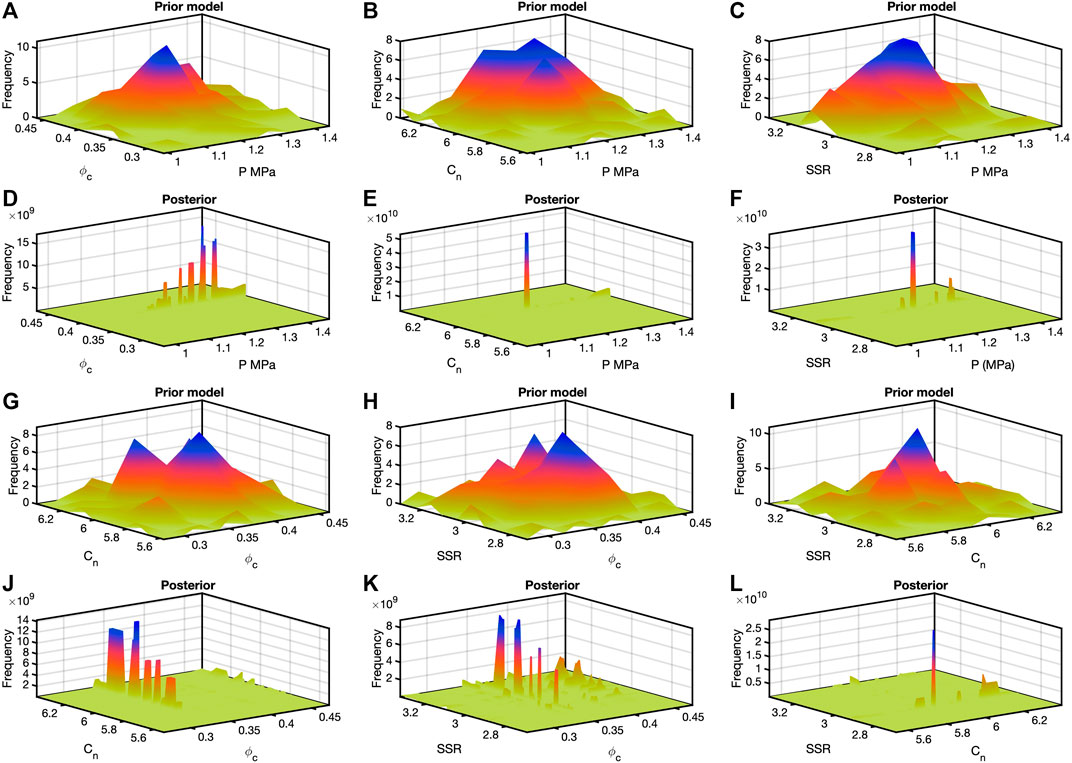
FIGURE 10. Soft-sand model and data set 1 results. Plots (A–C) are the bivariate prior model histograms for P versus ${\varphi }_c$, C_n, and SSR, respectively. Plots (D–F) contain the corresponding posterior histograms. Prior model histograms for ${\varphi }_c$- C_n, ${\varphi }_c$-SSR, and C_n -SSR are in (G), and their corresponding posteriors are in (J–L). Several peaks are present in (D). A high-frequency peak is present in (E,F). Multiple peaks are apparent in (J,K) for a narrow range of ${\varphi }_c$ and wide ranges of C_n and SSR. In (L) is one high-frequency peak.

An additional application for data set 1 was to run 100 trials of each rock-physics model. Within each trial, a different m was generated. The mean and covariance matrix were the same each time, but the randomly generated values for each trial were different. The results from each trial are the sets of bivariate histograms such as those in Figures 8–10. Values for inputs at maximum frequencies were selected from the appropriate bivariate posterior for each trial. For the modified Reuss, the cross plot in Figure 11A shows little to no correlation between ${\varphi }_0$ and $M_{df}$. Figure 11B shows the selected data, the starting model (black), a selection of prior models (blue), and the 100 MAP models (gray). The high-frequency values for the points in Figure 11A and thus the MAP models in Figure 11B came from Figure 8B.

FIGURE 11

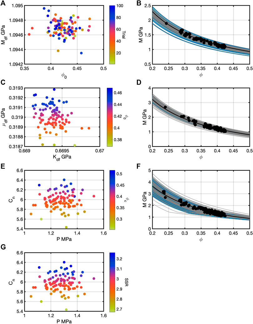
FIGURE 11. The pair of ${\varphi }_0$ and $M_{df}$ at the highest frequency was extracted for each of 100 trials using the modified Reuss model with data set 1. Those are plotted in (A) color coded by the trial number. A clear correlation is present. Using each pair, 100 MAP models were computed and are shown in (B) (gray) along with a selection of prior models in blue and the starting model in black. The same procedure was performed for the modified HS model. In (C) is the plot of ${\varphi }_0$- $K_{df}$ color coded by ${\mu }_{df}$. Correlation among the three terms is apparent. Starting, prior, and MAP models for these data points are in (D). Last, 100 trials of the soft-sand model were computed. In (E), the P-$C_n$ plot is color coded by ${\varphi }_c$. The corresponding MAP models and some prior models are in (F). In (G) is the for P-$C_n$ plot color coded by SSR. Correlations among the three parameters are observable in (E,G).

Similarly for the modified HS model, Figure 11C shows the scatter plot of $K_{df}$-${\mu }_{df}$ color-coded by ${\varphi }_0$. The $K_{df}$-${\mu }_{df}$ pair was extracted from Figure 9F; To determine ${\varphi }_0$, the maximum frequency value was selected from Figure 9D. This value could have been selected from Figure 9B, but the frequencies in Figure 9D were larger. Clear correlation among all three terms is evident, which was not clear when looking at only at the posterior bivariates alone. A subset of prior models, the 100 MAP models, and the selected data are in Figure 11D. Last, results for the 100 soft-sand trials are in Figures 11E–G. Figure 11E is the scatter plot of P-$C_n$, color-coded by ${\varphi }_c$. Figure 11F contains the selected data, some prior models (blue), and the MAP models. The plot in Figure 11G is P-$C_n$, color-coded by $SSR$. In Figures 11E,G, the three terms are correlated. For the points in Figure 11A, the P-${\varphi }_c$ pair was selected from Figure 10D, $C_n$ from Figure 10E, and $SSR$ from Figure 10F.

We applied the Bayesian framework to data set 2 using each of the rock-physics models. The sizes of m stay the same as they were for applications to data set 1. The general appearance of the results for data set 2 is much like the posterior bivariate histogram for data set 1. Thus, we do not display them here.

Finally, each rock-physics model was applied to data set 2 in 100 independent trials. Each trial introduced a different random m but with the same mean and covariance matrix. Values of the inputs were selected from the posterior histograms as described for the MAP models in 11. Figure 12 contains the scatter plots of the inputs and the 100 posterior models. Figure 12A shows the lack of correlation between ${\varphi }_0$ and $M_{df}$, and Figure 12B shows the selected data, some prior models, and the MAP models from those pairs of ${\varphi }_0$ and $M_{df}$ for the modified Reuss application. Figures 12C,D are the scatter plots and data and models, respectivley, for the modified HS application. The correlations among the three parameters are similar to what are shown in Figure 11C. Figures 12E–G are the plots for the soft-sand model, where again correlations are apparent among those model inputs. Figure 12E is color coded by ${\varphi }_c$ and Figure 12G by SSR.

FIGURE 12

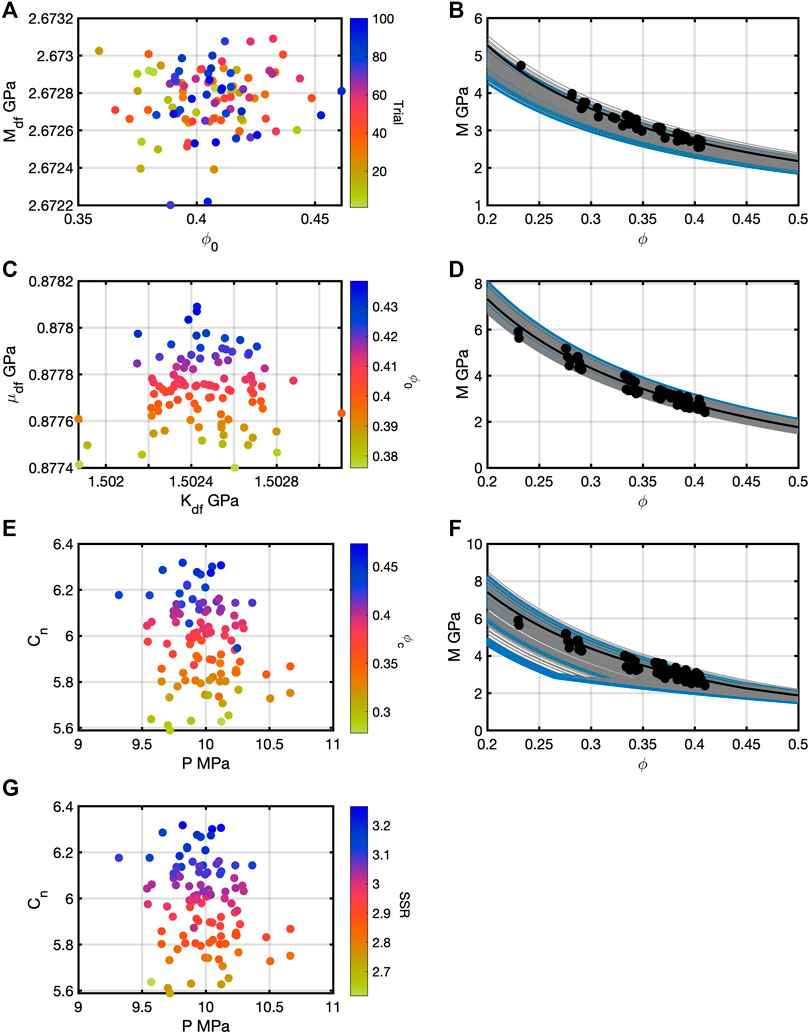
FIGURE 12. After 100 trials for the three models for data set 2, the highest frequency pairs were extracted as in Figure 11 for data set 1. (A) corresponds to the extracted values; (B) contains the starting model (black), a subset of prior models (blue), and MAP models (gray) for the modified Reuss. (C,D) contain those for the modified HS model. (E–G) contain those for the soft-sand model. Correlations are easily identifiable in the modified HS and soft-sand model parameters.

Discussion

The results of the Bayesian framework for the all the rock-physics models indicate correlations among their inputs that were not known previously. Specific to the R model, all three terms are correlated (Figures 6A, 7A). These correlations are not apparent when looking at the equation of the model, the sensitivities, or by looking at one set of bivariate histograms (e.g., Figure 3). After multiple trials each with a different m, the correlation pattern emerges. These correlations show up with both data sets but of course with different values for the three terms. Similar arguments can be made for the FS and HB models. Any given set of posterior histograms provides for an optimally fit model. Only after conducting many trials do the correlations among the inputs become evident. For these three models, all could be recast as linear in the log-log domain. The data could be plotted in the that domain as well, and the Bayesian analysis could have been performed in terms of fitting a line in the log-log domain. We did not do this because the velocity sensitivity as a function of pressure cannot be captured fully in the log-log domain.

When the covariance matrix of m was tested by trial and error for the three models, the R model was the easiest among the three models to find suitable values for the matrix. This situation likely occurred because A and B are coefficients, and n is an exponent. In the other two models, S is a coefficient, and n and k are exponents. The MAP models in Figures 6, 7 indicate this pattern. In Figure 6 especially, the posterior models for the R model clearly are better matches to the data than for the FS and HB models. In Figure 7, arguably all three sets of MAP models show about the same amount of scatter at higher pressures. The Merritt data set had nearly twice the number of data points as the Galveston Bay data set, and many more points are present at lower pressures, so a slight bias in fitting exists for the lower pressure data points.

Specific to the modified Reuss model, the two inputs are not clearly correlated (Figures 11A, 12A). After 100 trials each with a different m, no correlation pattern becomes clear with both data sets although different values for the two terms change. Correlations among the three inputs of the modified HS model emerged after the 100 trials. Within each trial, the appearances of the posterior histograms were similar with a lone high-frequency peak in the $K_{df}$-${\mu }_{df}$ pair and narrow value of ${\varphi }_0$ for a wide range of the others. From trial-to-trial, the location of the lone peak changed as did the narrow range of ${\varphi }_0$. Thus, some correlation could be inferred from the histograms but not as clearly as in the plots in Figures 11C, 12C. Given the bivariate posterior histograms, the relative significance of the inputs would be $K_{df}$ and ${\mu }_{df}$ first and then ${\varphi }_0$. With four inputs into the soft-sand model, the correlations that emerged were not anticipated. Nonetheless, the patterns in Figures 11, 12 indicate those correlations. In terms of relative significance, P and $C_n$ would be first, followed by $SSR$ and last, ${\varphi }_c$ However, that order could be changed. The modified Reuss and modified HS models could be recast as linear functions through simple substitutions. However, the same cannot be done for the data, so the Bayesian analysis must be done in the porosity-modulus domain.

When using these porosity-dependent rock-physics models with two, three, and four parameters, obviously providing two inputs versus three or four is easier. These models, used in a porosity-dependent manner, help to estimate porosities from velocity not observed in a data set. Of the three, one question that could arise would be which one is the most reliable? A potential answer could be inferred from the MAP models in Figures 11, 12. In both figures for the two data sets, the modified HS posterior models show the least scatter among themselves. Extrapolation to lower porosities might be more reliable from this model relative to the modified Reuss and soft-sand models. That said, if these models were used in studies that dealt with variable compositions and fluid saturations, they would need to be examined in the Bayesian framework with an appropriate data set.

This study identifies correlations among input parameters of pressure- and porosity-dependent rock-physics models. The Bayesian framework provided the means to establish these correlations. In a seismic-inversion or reservoir-characterization scheme, these correlations could be used to construct informative prior distributions. A user of any of the models examined here should be aware of these correlations. Exact values of the inputs will vary depending on the particular data set, but at least some simple templates could be defined to guide the setting of the values. Additional pressure- and porosity-dependent models should be examined using the Bayesian framework because the results obtained here might not be exactly relevant for other models. Furthermore, other types of rock-physics models, such as inclusion-based or excess-compliance models, would have to be examined in a similar fashion using appropriate data sets.

Data Availability Statement

Publicly available datasets were analyzed in this study. This data can be found here: doi:10.1190/1.2399459 and doi:10.1190/1.2364849.

Author Contributions

KS wrote the codes, the article, and generated the figures MS provided initial motivation for the work, edited the articles, and critiqued the results.

Conflict of Interest

The authors declare that the research was conducted in the absence of any commercial or financial relationships that could be construed as a potential conflict of interest.

Publisher’s Note

All claims expressed in this article are solely those of the authors and do not necessarily represent those of their affiliated organizations, or those of the publisher, the editors, and the reviewers. Any product that may be evaluated in this article, or claim that may be made by its manufacturer, is not guaranteed or endorsed by the publisher.

References

Avseth, P., Mukerji, T., and Mavko, G. (2005). Quantitative Seismic Interpretation: Applying Rock Physics Tools to Reduce Interpretation Risk. Cambridge, England: Cambridge University Press, 359.

Google Scholar

Ba, J., Cao, H., Carcione, J. M., Tang, G., Yan, X.-F., Sun, W.-t., et al. (2013). Multiscale Rock-Physics Templates for Gas Detection in Carbonate Reservoirs. J. Appl. Geophys. 93, 77–82. doi:10.1016/j.jappgeo.2013.03.011

CrossRef Full Text | Google Scholar

Bosch, M., Mukerji, T., and Gonzalez, E. F. (2010). Seismic Inversion for Reservoir Properties Combining Statistical Rock Physics and Geostatistics: A Review. Geophysics 75 (5), 75A165–75A176. doi:10.1190/1.3478209

CrossRef Full Text | Google Scholar

Buland, A., and Omre, H. (2003). Bayesian Linearized AVO Inversion. Geophysics 68 (1), 185–198. doi:10.1190/1.1543206

CrossRef Full Text | Google Scholar

de Figueiredo, L. P., Grana, D., Bordignon, F. L., Santos, M., Roisenberg, M., and Rodrigues, B. B. (2018). Joint Bayesian Inversion Based on Rock-Physics Prior Modeling for the Estimation of Spatially Correlated Reservoir Properties. Geophysics 83, M49–M61. doi:10.1190/geo2017-0463.1

CrossRef Full Text | Google Scholar

de Figueiredo, L. P., Grana, D., Roisenberg, M., and Rodrigues, B. B. (2019). Multimodal Markov Chain Monte Carlo Method for Nonlinear Petrophysical Seismic Inversion. Geophysics 84, M1–M13. doi:10.1190/geo2018-0839.1

CrossRef Full Text | Google Scholar

de Figueiredo, L. P., Grana, D., Santos, M., Figueiredo, W., Roisenberg, M., and Schwedersky Neto, G. (2017). Bayesian Seismic Inversion Based on Rock-Physics Prior Modeling for the Joint Estimation of Acoustic Impedance, Porosity and Lithofacies. J. Comput. Phys. 336, 128–142. doi:10.1016/j.jcp.2017.02.013

CrossRef Full Text | Google Scholar

Dvorkin, J., and Nur, A. (1996). Elasticity of High‐porosity Sandstones: Theory for Two North Sea Data Sets. Geophysics 61 (5), 1363–1370. doi:10.1190/1.1444059

CrossRef Full Text | Google Scholar

Fam, M., and Santhamarian, J. C. (1997). A Study of Consolidation Using Mechanical and Electromagnetic Waves. Géotechnique 47, 203–219. doi:10.1680/geot.1997.47.2.203

CrossRef Full Text | Google Scholar

Grana, D. (2020). Bayesian Petroelastic Inversion with Multiple Prior Models. Geophysics 85 (5), M57–M71. doi:10.1190/GEO2019-0625.1

CrossRef Full Text | Google Scholar

Grana, D., Fjeldstad, T., and Omre, H. (2017). Bayesian Gaussian Mixture Linear Inversion for Geophysical Inverse Problems. Math. Geosci. 49, 493–515. doi:10.1007/s11004-016-9671-9

CrossRef Full Text | Google Scholar

Grana, D. (2018). Joint Facies and Reservoir Properties Inversion. Geophysics 83, M15–M24. doi:10.1190/geo2017-0670.1

CrossRef Full Text | Google Scholar

Grana, D., Mukerji, T., and Doyen, P. (2021). Seismic Reservoir Modeling: Theory, Examples, and Algorithms. Hoboken, New Jersey: Wiley-Blackwell, 272.

Google Scholar

Hardin, B. O., and Blandford, G. E. (1989). Elasticity of Particulate Materials. J. Geotechnical Eng. 115, 788–805. doi:10.1061/(ASCE)0733-941010.1061/(asce)0733-9410(1989)115:6(788)

CrossRef Full Text | Google Scholar

Jullum, M., and Kolbjørnsen, O. (2016). A Gaussian-Based Framework for Local Bayesian Inversion of Geophysical Data to Rock Properties. Geophysics 81, R75–R87. doi:10.1190/GEO2015-0314.1

CrossRef Full Text | Google Scholar

Kemper, M., and Gunning, J. (2014). Joint Impedance and Facies Inversion - Seismic Inversion Redefined. First Break 32 (9), 89–95. doi:10.3997/1365-2397.32.9.77968

CrossRef Full Text | Google Scholar

Mavko, G., Mukerji, T., and Dvorkin, J. (2020). The Rock Physics Handbook. Third edition. Cambridge, England: Cambridge University Press, 727.

Google Scholar

Mindlin, R. D. (1949). Compliance of Elastic Bodies in Contact. Trans. ASME 71, A–259. doi:10.1115/1.4009973

CrossRef Full Text | Google Scholar

Nawaz, M. A., Curtis, a., Shahraeeni, M. S., and Gerea, C. (2020). Variational Bayesian Inversion of Seismic Attributes Jointly for Geologic Facies and Petrophysical Rock Properties. Geophysics 85 (4), MR213–MR233. doi:10.1190/GEO2019-0163.1

CrossRef Full Text | Google Scholar

Pang, M., Ba, J., Carcione, J. M., Picotti, S., Zhou, J., and Jiang, R. (2019). Estimation of Porosity and Fluid Saturation in Carbonates from Rock-Physics Templates Based on Seismic Q. Geophysics 84, M25–M36. doi:10.1190/GEO2019-0031.1

CrossRef Full Text | Google Scholar

Pang, M., Ba, J., Carcione, J. M., Zhang, L., Ma, R., and Wei, Y. (2021). Seismic Identification of Tight-Oil Reservoirs by Using 3D Rock-Physics Templates. J. Pet. Sci. Eng. 201, 108476. doi:10.1016/j.petrol.2021.108476

CrossRef Full Text | Google Scholar

Ray, A., Alumbaugh, D. L., Hoversten, G. M., and Key, K. (2013). Robust and Accelerated Bayesian Inversion of marine Controlled-Source Electromagnetic Data Using Parallel Tempering. Geophysics 78 (6), E271–E280. doi:10.1190/geo2013-0128.1

CrossRef Full Text | Google Scholar

Rimstad, K., Avseth, P., and Omre, H. (2012). Hierarchical Bayesian Lithology/fluid Prediction: A North Sea Case Study. Geophysics 77, B69–B85. doi:10.1190/geo2011-0202.1

CrossRef Full Text | Google Scholar

Robertson, P. K., Sasitharan, S., Cunning, J. C., and Sego, D. C. (1995). Shear-Wave Velocity to Evaluate In-Situ State of Ottawa Sand. J. Geotechnical Eng. 121, 262–273. doi:10.1061/(ASCE)0733-941010.1061/(asce)0733-9410(1995)121:3(262)

CrossRef Full Text | Google Scholar

Sen, M. K. (2006). Seismic Inversion. Richardson, TX: Society of Petroleum Engineers, 120.

Google Scholar

Sen, M. K., and Stoffa, P., L. (2013). Global Optimization Methods in Geophysical Inversion. Second edition. Cambridge, England: Cambridge University Press, 289.

Google Scholar

Sen, M. K., and Stoffa, P. L. (1996). Bayesian Inference, Gibbs' Sampler and Uncertainty Estimation in Geophysical Inversion1. Geophys. Prospect 44, 313–350. doi:10.1111/j.1365-2478.1996.tb00152.x

CrossRef Full Text | Google Scholar

Spikes, K., Mukerji, T., Dvorkin, J., and Mavko, G. (2007). Probabilistic Seismic Inversion Based on Rock-Physics Models. Geophysics 72 (5), R87–R97. doi:10.1190/1.2760162

CrossRef Full Text | Google Scholar

Tarantola, A. (2005). Inverse Problem Theory and Methods for Model Parameter Estimation. Paris, France: Society for Industrial and Applied Mathematics, 352.

Google Scholar

Ulrych, T. J., Sacchi, M. D., and Woodbury, A. (2001). A Bayes Tour of Inversion: A Tutorial. Geophysics 66 (1), 55–69. doi:10.1190/1.1444923

CrossRef Full Text | Google Scholar

Zimmer, M. A., Prasad, M., Mavko, G., and Nur, A. (2007a). Seismic Velocities of Unconsolidated Sands: Part 1 - Pressure Trends from 0.1 to 20 MPa. Geophysics 72, E1–E13. doi:10.1190/1.2399459

CrossRef Full Text | Google Scholar

Zimmer, M. A., Prasad, M., Mavko, G., and Nur, A. (2007b). Seismic Velocities of Unconsolidated Sands: Part 2 - Influence of Sorting- and Compaction-Induced Porosity Variation. Geophysics 72, E15–E25. doi:10.1190/1.2364849

CrossRef Full Text | Google Scholar

Zimmer, M. A. (2003). Seismic Velocities in Unconsolidated Sands: Measurements of Pressure, Sorting, and Compaction Effects. Ph.D. dissertationStanford University.

Google Scholar