Semi-Supervised Learning–Based Petrophysical Facies Division and “Sweet Spot” Identification of Low-Permeability Sandstone Reservoir

The identification of the “sweet spot” of low-permeability sandstone reservoirs is a basic research topic in the exploration and development of oil and gas fields. Lithology identification, reservoir classification based on the pore structure and physical properties, and petrophysical facies classification are common methods for low-permeability reservoir classification, but their classification effect needs to be improved. The low-permeability reservoir is characterized by low rock physical properties, small porosity and permeability distribution range, and strong heterogeneity between layers. The seepage capacity and productivity of the reservoir vary considerably. Moreover, the logging response characteristics and resistivity value are similar for low-permeability reservoirs. In addition to physical properties and oil bearing, they are also affected by factors such as complex lithology, pore structure, and other factors, making it difficult for division of reservoir petrophysical facies and “sweet spot” identification. In this study, the logging values between low-porosity and -permeability reservoirs in the Paleozoic Es₃ reservoir in the M field of the Bohai Sea, and between natural gamma rays and triple porosity reservoirs are similar. Resistivity is strongly influenced by physical properties, oil content, pore structure, and clay content, and the productivity difference is obvious. In order to improve the identification accuracy of “sweet spot,” a semi-supervised learning model for petrophysical facies division is proposed. The influence of lithology and physical properties on resistivity was removed by using an artificial neural network to predict resistivity R₀ saturated with pure water. Based on the logging data, the automatic clustering MRGC algorithm was used to optimize the sensitive parameters and divide the logging facies to establish the unsupervised clustering model. Then using the divided results of mercury injection data, core cast thin layers, and logging faces, the characteristics of diagenetic types, pore structure, and logging response were integrated to identify rock petrophysical facies and establish a supervised identification model. A semi-supervised learning model based on the combination of “unsupervised supervised” was extended to the whole region training prediction for “sweet spot” identification, and the prediction results of the model were in good agreement with the actual results.

Introduction

As exploration and development progress, the research objective of logging interpretation gradually shifts to complex reservoirs such as low porosity and low permeability. The seepage capacity and productivity of these reservoirs are affected by many factors, and the productivity varies greatly. Therefore, it is of great significance for the identification of low-permeability reservoirs. The production capacity of oil and gas reservoirs is mainly affected by many factors such as lithology, physical properties, oil content, shale content, and pore structure. However, production capacity is a combination of various influencing factors. With the advantages of high wellbore resolution and strong multi-well comparability, the logging method is the main means of “sweet spot” identification. Logging response can, to some extent, directly reflect the lithology, physical properties, seepage characteristics, and production capacity of oil and gas reservoirs. However, the similarity in response characteristics of the logging methods for low-permeability reservoirs and the high and low values of resistivity are not only affected by fluid properties, which bring new challenges to reservoir classification and “sweet spot” identification. Therefore, in order to predict the hydrocarbon distribution law and dominant reservoir of low-permeability sandstone reservoirs, reservoir classification based on integrating logging response, diagenetic type, and pore structure is very important. Lithology identification, reservoir classification based on pore structure and physical property characteristics, and petrophysical facies division are common methods for low-permeability reservoir classification research. They establish reservoir identification charts from different angles and mechanisms. There are several types of existing reservoir classification criteria, and they vary from region to region to provide guidance for the exploration and development of low-permeability oil fields (Sun, 2016).

Rock petrophysical facies is a genetic unit of reservoir with similar diagenesis. It is the comprehensive effect of sedimentation, diagenesis, reservoir formation, and later structure, which can better reflect the rock characteristics. Identifying different diagenetic types and hence the delineation of petrophysical facies is of great significance to predict favorable reservoir and “sweet spot” distribution in low-permeability sandstone reservoir (Lu and Liu, 2012). From the perspective of “facies control,” Lai Jin et al. (Jin et al., 2013a; Jin et al., 2013b; Jin et al., 2015; Lai, 2016 ) proposed that petrophysical facies are mainly controlled by sedimentary facies, diagenetic facies, and fracture facies (Gong et al., 2019; Gong et al., 2021), and their classification and naming should adopt the principle of superposition of three types of facies, namely, sedimentary facies + diagenetic facies + fracture facies. Wang Bin (Wang, 2018) divided sedimentary microfacies according to well logging, coring, mud logging, and other data. On the basis of well logging identification and induction, the distribution law of diagenetic facies in the vertical direction of the well section was identified by using the information from the combination of log data. On this basis, the petrophysical facies of the well was divided and named by superposition. In order to more accurately predict the distribution of high-quality reservoirs and the differences in internal reservoir properties, Chai and Wang (2016) and others studied the four main controlling factors of lithology, lithofacies, diagenetic facies, fracture facies, and pore structure of a tight sandstone reservoir of the second member of the Xujiahe Formation in the Anyue area, central Sichuan, following the concept of petrophysical facies, using core, thin layer, mercury injection and logging data. The logging characterization method and logging identification standard were established, and on this basis, the classification of petrophysical facies and quantitative evaluation standard of reservoirs were put forward.

Huang et al. (2017) proposed a comprehensive evaluation and interpretation method of reservoir logging based on petrophysical research, which combined the main control factors such as macro-sedimentation, diagenesis, and structure with the micro-rock characteristics, physical properties, and pore throat structure characteristics, so that the logging interpretation has a stronger comprehensive guiding significance and have got rid of the limitations of “one hole view.” Shi et al. (2005) have found that rock petrophysical facies is the dominant factor controlling the “four properties” relationship and logging response characteristics of low-permeability lithologic reservoirs. Establishing a model for interpreting logging reservoir parameters based on petrophysical facies classification is an effective method to improve the logging interpretation accuracy of low-permeability and heterogeneous reservoirs.

Yao et al. (1995) believed that petrophysical facies is a complex of reservoir physical properties, which reflects the pore structure information under the influence of sedimentation, diagenesis, and microfractures. They classified petrophysical facies based on equations such as the flow unit index and reservoir quality index, thus improving the accuracy of permeability prediction. Soete et al. (2014) took 8 wells in the Paleozoic study area of the Irish Sea as an example, by calculating and comparing the porosity, permeability, clay volume, and other parameters of each well and dividing different petrophysical facies types to find the better dominant formation of the reservoir. With the rise of intelligent emerging technology, artificial intelligence logging evaluation technology has also emerged. Neural networks, machine learning, automatic clustering, and other intelligent algorithms are also being developed in the field of well logging, which greatly improves the efficiency of reservoir classification and the accuracy of “sweet spot” identification. Shi et al. (2018) combined with geological, logging, and core casting thin section data and successfully divided the logging facies by the graph theory multi-resolution clustering algorithm. Compared with the traditional method, the calculation accuracy was significantly improved, the corresponding relationship between logging facies and lithofacies in the study area was determined, and a permeability evaluation model based on logging facies constraint was established. Zhang Meng (Zhang, 2018) used the nuclear attraction theory in the MRGC method to initially obtain the rough classification results of lithology, and then used the SOM algorithm and dynamic neuron splitting technology to achieve coarse to fine classification of lithology according to the multilevel classification scheme provided by the MRGC method. Grana et al. (2012) proposed the formation, evaluation, and analysis of petrophysical model division. Petrophysical properties of the reservoir were studied by the combination of lithofacies classification and other methods. Based on the traditional stratigraphic evaluation model and cluster analysis technology, a complete Monte Carlo method was introduced to participate in the evaluation to find the relationship between petrophysical properties, elastic properties, and facies, so as to divide rock petrophysical facies. Li and Li (2013) combined k-means algorithm and self-organizing feature mapping to identify lithofacies. Researchers have also proposed task-driven data mining with domain knowledge. Leite et al. (2013) used classification models such as multilayer perceptron, SVM, k-nearest neighbor, and other classification models, and integrated classifiers by bagging and boosting to identify rock layers. Ye and Rabiller (2000) solved the parameter sensitive problem caused by “dimension” through an automatic clustering MRGC algorithm and compared the phase classification results with the nuclear magnetic T2 spectrum. It was found that the classification results were basically consistent with the actual results. Lifei et al. (2021) have carried out extensive experiments on real logging data and found that the semi-supervised learning algorithm can obtain relatively accurate lithology prediction effect by mining the distribution characteristics contained in marked data and unmarked data. Taking Paleogene Es₃ of M oilfield in Bohai Sea as an example, a semi-supervised learning model for petrophysical facies division was proposed to better divide the petrophysical facies and “sweet spot” identification with the help of the difference in petrophysical characteristics of the formation logging data, in response to the difficulty of “sweet spot” identification in a low-permeability sandstone reservoir. Based on the mercury injection data, the petrophysical facies of the coring section was analyzed, and then the combination of “unsupervised supervised” was extended to the whole region training prediction for “sweet spot” identification, so as to realize the petrophysical facies discrimination of the whole well section; we analyzed the porosity permeability relationship based on the classification of petrophysical facies. The predictions of the model have proved to be in good agreement with the actual results, which is of great significance to find the “sweet spot area” of low-permeability sandstone reservoirs.

Regional Overview

The Palaeozoic M field in the Bohai Sea is geographically located at the western end of Bonan low uplift and the boundary between Bozhong sag and Huanghekou sag. The structural strike is mainly EW and NE, and multiple faults are developed. The faults cut each other, the shape is complex, and the faults determine the oil–water distribution. On the whole, it presents the reservoir characteristics of upper oil and lower water. Drilling shows that this well area is one of the most favorable oil and gas enrichment areas in the Bohai Sea, which has superior geological conditions for oil and gas accumulation. The main development layer series of the oilfield is the Shahejie Formation, and the buried depth of the reservoir is 3200–3900 m. The third member of the Shahejie Formation is a fan-shaped deltaic turbidite deposit, with wide distribution of rock grain size and low maturity. It is mainly lithic arkose and feldspathic lithic sandstone, with sub-prismatic roundness and relatively poor sorting. The porosity (PORE) is mainly 3.3–17.9%, and the permeability (PERM) is mainly 0.01–25.4 md, and it is a medium-porosity, low-permeability and ultralow-permeability reservoir. These reservoirs are lithologically dense, with small pores, fine throat, poor pore throat connectivity, obvious productivity difference, and difficult identification of “sweet spots.” As an example, the four reservoirs with significant production differences in the four key wells selected (Figures 1, 2 and Table 1) yielded 106, 14.52, 3.25, and 0.83 m³, respectively. It can be found from the prepared logging response curve and logging response characteristic summary table (Figure 1 and Table 1): the logging response of the four oil layers is similar except resistivity, porosity, and permeability. The three-porosity logging values [acoustic (AC), neutron (CNL), and density (DEN)] are similar. The average AC values of the four oil layers are 75.69, 74.30, 75.00, and 62.10 US/FT, respectively; the average CNL values are 0.16, 0.12, 0.12, and 0.07 V/V, respectively; and the average den values are 2.45, 2.44, 2.40, and 2.53 g/m³, respectively. In addition to the low value of ① oil layer (61.94 API), the gamma (GR) mean values of the other three oil layers are not different, which are 85.98, 91.54, and 83.94 API, respectively. The difference of resistivity value is relatively obvious. In addition to the influence of oil and gas, pore structure, physical properties, and clay will affect the resistivity. Poor physical properties and complex pore structure will increase the resistivity, while high clay content will decrease the resistivity. The average values of the four oil layers of deep investigate lateral resistivity (RD) are 107.96, 20.41, 38.63, and 80.21 OHMM, respectively. From the observation of the cross-plot of porosity and permeability (Figure 2), on the whole, the porosity and permeability distribution trend of the four oil layers basically presents a straight line with an angle of 60 degrees, and the porosity and permeability correlation is good; when the four oil layers are intersected, it can be found that the porosity and permeability difference of the four small layers is obvious: the porosity and permeability of oil layer ① is the highest, and the porosity of oil layer ② is basically the same as that of oil layer ③, but the permeability of oil layer ② is higher than that of oil layer ③, and the porosity and permeability of oil layer ④ is the worst: the permeability is basically below 0.1 mdc.

FIGURE 1

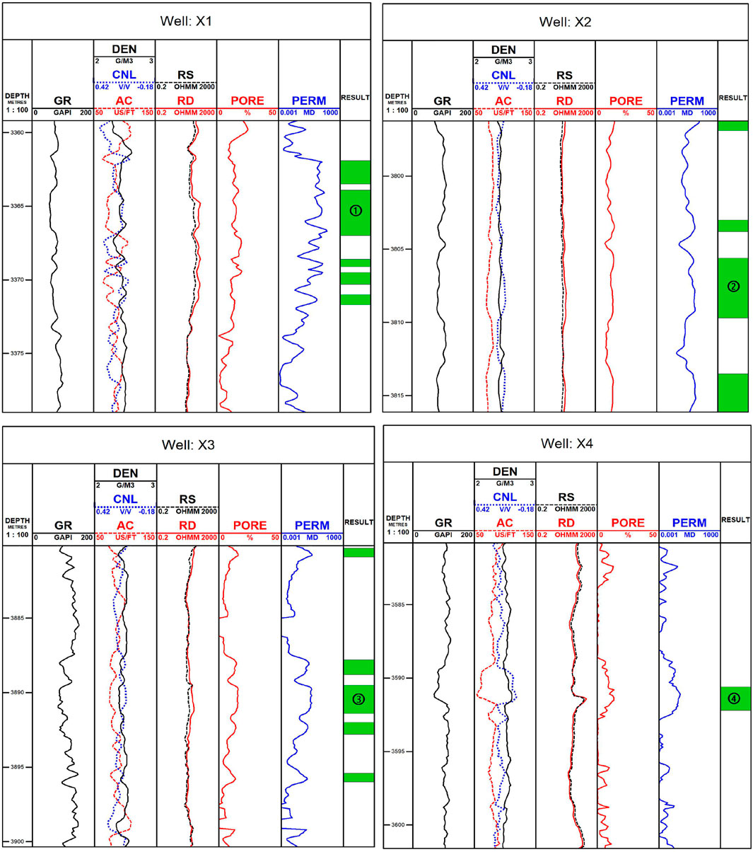
FIGURE 1. Logging response curve of Es₃ (Gamma ray log (GR), Density log (DEN), Compensated neutron log (CNL), Acoustic log (AC), Shallow lateral resistivity log (RS), Deep lateral resistivity log (RD), Porosity log (PORE), Permeability log (PERM), Fluid properties (RESULT), the same below).

FIGURE 2

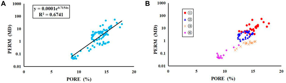
FIGURE 2. Cross-plot of porosity and permeability of small layer 4 of the Es₃ reservoir [(A): overall cross-plot of small layer 4; (B): separate cross-plot of small layer 4].

TABLE 1

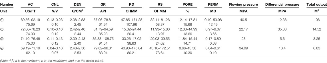
TABLE 1. Logging response characteristic summary table of 4 small layers in the Es₃ reservoir.

Prediction of Saturated Pure Water Resistivity R₀ by Artificial Neural Network Despite the Influence of Lithology and Physical Properties on Resistivity

Resistivity Value of Saturated Pure Water R₀

Using formation resistivity to analyze the variability of the actual formation is difficult due to the similar logging response in low-permeability reservoirs, the similar range of values taken for natural gamma rays and triple holes, and the fact that resistivity is influenced by a number of factors. In addition to the influence of oil and gas, the resistivity will be affected by pore structure, physical properties, and clay. Poor physical properties and complex pore structure will lead to the increase of resistivity, and high clay content will cause the decline of the resistivity value. In order to eliminate the influence of these factors on the reservoir resistivity value, it is necessary to calculate the saturated pure water resistivity (R₀). In conventional oil reservoirs, the R₀ value is usually calculated by the Archie formula or an argillaceous sandstone conductivity model formula (Li and Ying, 2012), but the pore structure of the low-permeability tight reservoir is complex, and the R₀ value calculated by the aforementioned method is often inaccurate, making it difficult to find the law of model parameters. Therefore, this study adopts the method of machine learning to learn and predict, selects a key well, and takes the resistivity value of the pure water section of the well as the saturated pure water resistivity R₀’s training set, so as to conduct modeling training to predict the R₀ value of the whole well section.

The resistivity R₀ value of saturated pure water predicted by the neural network was superimposed with the formation deep lateral resistivity RD value. The fluid properties can be judged according to the amplitude difference and curve change direction, which provided a basis for “sweet spot” evaluation. When the amplitude of the R₀ curve and RD curve of permeable layer coincided, the reservoir was interpreted as water layer; When the R₀ curve of the permeable layer was significantly smaller than the amplitude of the RD curve, the reservoir was an oil layer; When the R₀ curve was much higher than the deep lateral resistivity curve RD and there was a peak, it could be identified as a dry layer. This is because most dry layers contain calcareous interlayer and its porosity is small, so the amplitude value of R₀ curve calculated according to the aforementioned formula is very large. Therefore, the question of whether the predicted R₀ value is correct can be controlled by comparing the two resistivity values of the oil and water layers to control the quality of the predicted R₀ value.

Artificial Neural Network Prediction R₀

The artificial neural network abstracts the human brain neural network from the perspective of information processing and establishes an operation model, which is composed of a large number of nodes (or neurons) connected with each other. Each node represents a specific output function, which is called an excitation function. The connection between each nodes represents the weighted value of the signal passing through the connection, which is called the weight, and it is equivalent to the memory of the artificial neural network. The output of the network varies depending on how the network is connected, the weight value, and the excitation function. Generally speaking, the selection of the excitation function is particularly important for the learning effect of data samples (Fang et al., 2011).

Therefore, Relu and Tanh were chosen as the activation functions for the different neural layers, taking into account the data characteristics of the input data (Guo and Gao, 1996; Wei et al., 2020). In the framework of the neural network, a three-layer neural network, one input layer, one hidden layer, and one output layer, was adopted. In this study, acoustic time difference AC, compensated neutron CNL, and density den and deep lateral resistivity Rd were selected as the input data and was input into the input layer after normalization. After fitting the data of the hidden layer, the resistivity R₀ saturated with pure water was used as the output layer. The data structure is as follows:

$X_{input}={\left\{\begin{array}{c}{x}_{11},x_{12},\cdot \cdot \cdot ,x_{1m}\\ \begin{array}{cccc}\cdot \cdot & \cdot \cdot & \cdot \cdot & \cdot \cdot \end{array}\\ x_{n1},x_{n2},\cdot \cdot \cdot ,x_{nm}\end{array}\right\}}^T={\left\{\begin{array}{c}A{C}_1,CN{L}_1,DE{N}_1,R{D}_1\\ \begin{array}{cccc}\cdot \cdot \cdot & \cdot \cdot \cdot & \cdot \cdot \cdot & \cdot \cdot \cdot \end{array}\\ A{C}_n,CN{L}_{\text{n}},DE{N}_n,R{D}_n\end{array}\right\}}^T,(1)$

$Y_{output}={\left(y_1,y_2,\cdot \cdot \cdot ,y_n\right)}^T={\left(R_{0_1},R_{0_2},\cdot \cdot \cdot ,R_{0_n}\right)}^T.(2)$

In Eq. 1, n is the number of training samples and m is the type of input parameters corresponding to each sample, so the number of inputs and outputs of the neural network are 4 and 1, respectively, and non-linear mapping completed by the network is f:Rⁿ→R¹. If the hidden layer is p, the input of each node in the hidden layer of the network is given as follows:

$S_j={\displaystyle \sum _{i=1}^m{w}_{ij}}{x}_i-{\theta }_j\left(j=\mathrm{1,2},\cdot \cdot \cdot p\right),(3)$

In the equation, w_ij is the connection weight from input layer to hidden layer and θ_j is the threshold of the hidden layer node.

When the input data, output data, activation function, and neuron layers are completely determined, the neural network architecture can be carried out. The neural network architecture for predicting the resistivity R₀ of saturated with pure water by an artificial neural network is shown in Figure 3.

FIGURE 3

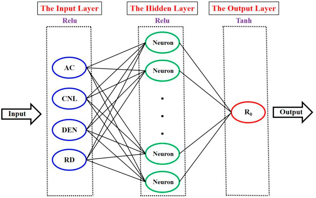
FIGURE 3. Structure diagram neural network of resistivity R₀ saturated with pure water predicted by the artificial neural network.

By analyzing resistivity value of the well section in the pure water layer using an artificial neural network, a model was established and learned, and the R0 value of the whole well section was obtained (Figure 4). Moreover, the resistivity R₀ value full of pure water predicted by the neural network was superimposed with the formation deep lateral resistivity RD value. According to the amplitude difference and curve change direction, the fluid property of the well was clearly judged and the oil–water interface was divided. By observing the superposition of the RD curve and RS curve and the superposition of the RD curve and R₀ curve, it can be found that the deep and shallow lateral resistivity curves always coincide and cannot show the difference of fluid properties; When the R₀ curve of the permeable layer was obviously smaller than the amplitude of the RD curve, the green filling with amplitude difference was interpreted as an oil layer. When the R₀ curve of the permeable layer basically coincided with the amplitude of the RD curve, the reservoir was interpreted as a water layer, and the oil–water interface is clearly divided. The results showed that the resistivity R₀ of saturated pure water predicted by the artificial neural network can remove well the influence of lithology and physical properties on resistivity. Compared with the actual results, the fluid property identification results with deep lateral resistivity superimposed were in good agreement, which provided a theoretical basis for “sweet spot” identification of low-permeability reservoirs with complex pore structure.

FIGURE 4

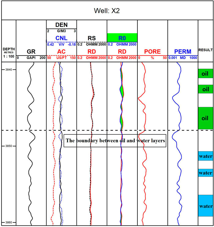
FIGURE 4. Result plots of resistivity R₀ of saturated pure water predicted by the artificial neural network.

Establishment of Rock Petrophysical Facies Identification Method Based on Semi-Supervised Learning

Information of petrophysical formation can be obtained from logging, including various physical and chemical properties of rocks, such as rock density, resistivity, hydrogen index, natural gamma ray, natural potential, and longitudinal wave propagation velocity, and can directly reflect the lithology, physical properties, reservoir properties, and production capacity of reservoirs to a certain extent. Different reservoirs have their own petrophysical characteristics. Logging and core analysis data can reflect the heterogeneity and the pore structure of the reservoir. However, due to the similar logging response of the low-permeability reservoir, the similar range of natural gamma ray and three-porosity values, and the high and low resistivity being influenced by multiple factors, it is difficult to analyze the changes of the actual formation by using the conventional logging data. It is found that the petrophysical facies controls the “four characteristics” relationship of low-permeability lithologic reservoirs and the dominant factor of logging response characteristics. “Sweet spot” identification based on petrophysical facies classification is an effective method to improve the logging interpretation accuracy of low-permeability and heterogeneous reservoirs. Based on this, a semi-supervised petrophysical facies identification method (Figure 5) was established, which combined an unsupervised clustering model with the supervised identification model. The unsupervised clustering model is used to input sensitive logging curves and divide logging facies by the automatic clustering algorithm, while the supervised identification model is used to recognize petrophysical facies by using mercury injection data, core cast thin section, logging facies division results, and other data, and thus realizing the function of petrophysical facies recognition of semi-supervised learning.

FIGURE 5

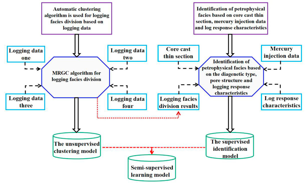
FIGURE 5. Flowchart of petrophysical facies division based on semi-supervised learning.

Automatic Clustering MRGC Algorithm for Logging Facies Division

A logging facies analysis involves selecting representative key coring wells, dividing logging facies through conventional logging curves of known lithology and strata, and determining the corresponding relationship between each logging facies and petrophysical facies. Based on this correspondence, a continuous layer-by-layer logging facies analysis was carried out for key wells and non-coring wells, and the petrophysical facies of each layer was determined. Finally, the petrophysical facies of all strata in these well sections were obtained. Generally speaking, the formation of a certain lithology in the same sedimentary environment has a specific set of logging parameter values. The formation of the whole drilling profile can be divided into several logging facies with geological significance by logging data. Reservoirs of similar logging facies generally have similar lithology, physical properties, pore structure, and logging response characteristics. Therefore, the study of reservoir logging facies can be used to better identify petrophysical facies by transforming the heterogeneity and non-linearity of complex reservoir into homogeneity and linearity.

However, in the data analysis of logging field, there are many kinds of index variables to choose, and the relationship between variables is complex. Clustering is used to solve the problem where explicit mathematical models are not considered and can effectively represent and predict uncertain and unstructured data. In this study, an automatic clustering algorithm (MRGC) was used to divide logging facies. As an unsupervised learning method, on the basis of absorbing the KNN algorithm, it delimits the nearest neighbor relationship between sampling points and integrates attraction set to realize classification (Tian et al., 2016; Wu et al., 2020).

Principle of MRGC Algorithm

The MRGC algorithm is characterized by each depth logging sample point using two indexes describing the adjacent relationship: the neighboring index (NI) and kernel representative index (KRI). Based on the relationship between NI and KRI, small natural data groups are formed, which may differ significantly in size, shape, separation, and quantity. Then the mutation in KRI corresponds to the optimal number of clusters at different resolutions. The optimal number of segments is determined by mutation of the decreasingly ordered KRI curves, thus enabling an automatic cluster analysis.

A neighboring index (NI) was used to divide logging facies (Gan, 1994). Let X be an element in set S, and y is the n-th adjacent value of x in the set S, n≤N. The relative rank of point x relative to its n-th NN, adjacent value y is defined as follows:

${\delta }_{\text{n}}\left(x\right)=\{\begin{array}{c}{e}^{\left(-m/\alpha \right)},ifxis{y}^{\text{'}}sm-thNN,m\le N-1;\\ b,ifxisnotbelongtothesetof{y}^{\prime }sKNN.\end{array},(4)$

where x has a finite rank relative to each minimum adjacent value (KNN) of x : δ n (n =1, 2,…, K). Let

$S\left(x\right)={\displaystyle \sum _{n=1}^N{\delta }_n}\left(x\right),(5)$

$S_{M\text{in}}=\underset{\begin{array}{c}i=1N\end{array}}{Min}\left\{S\left(x_i\right)\right\},(6)$

$S_{Max}=\underset{\begin{array}{c}i=1N\end{array}}{Max}\left\{S\left(x_i\right)\right\},(7)$

NI is determined by the normalized value of set S from 0 to 1, that is,

$NI\left(x\right)=\frac{S\left(x\right)-S_{Min}}{S_{Max}-S_{Min}},(8)$

In Eqs 4–8: N is the number of elements in S set and α is the smoothing coefficient, a>0; when b ≤ N-1, b is the estimated value of the rank of the adjacent value x of y; δ n is the rank of the adjacent value x of y, which is a decreasing function strictly varying from 1 to 0. When m = 0, δ n = 1, the higher the value of M, δ n approaches 0, but δ n is never equal to 0. Therefore, the higher the NI value, the closer the point is to the core of the cluster.

The number of optimal classes is actually a function of “resolution,” that is, the clustering results with more classification results (high-resolution) are subdivided by a category in the clustering results with less classification results (low-resolution), and then the optimal class can be selected according to the actual needs.

The kernel representative index (KRI) is a combined function of the neighborhood index NI (x), the number of neighbors m (x, y), and the distance function d (x, y), that is,

$KRI\left(x\right)=NI\left(x\right)M\left(x,y\right)D\left(x,y\right),(9)$

In Eq. 9: M(x,y) = n; y is the nth adjacent value of x; and D (x, y) is the distance from point x to point y.

NI (x) can be used to identify the kernel of a clustering result. The number of neighbors M (x, y) tends to produce data sets of the same scale, while the distance function D (x, y) tends to produce data sets of the same volume. The combination of M (x, y) and D (x, y) can therefore achieve a good balance in the data scale and volume and produce consistent results, that is, the best logging results can be selected. When the KRI is arranged in a descending order, a change from one steady state to another results in a corresponding number of inflection points, which correspond to different kinds of clustering results. At the same time, the local maximum (i.e., inflection point) of the gradient curve is calculated, and the points corresponding to the maximum KRI are selected to form the final clustering result (Figure 6).

FIGURE 6

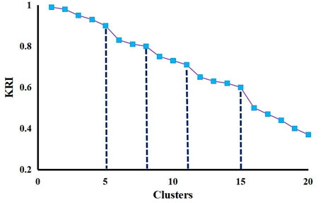
FIGURE 6. Schematic diagram of determining the optimal number of logging facies by the KRI.

Division of Logging Facies Flow by Automatic Clustering MRGC Algorithm

The logging facies division of the automatic clustering algorithm (MRGC) roughly has the following process: first, a key well with more coring was selected, and uniform distribution of coring sections was as much as possible. The key wells with complete logging curve and distinct electrical characteristics that are representative of the whole area were used as standard wells for modeling. Then logging curves with different parameter combinations were input as learning curves. Due to different data types measured by different logging methods, their dimensions and numerical magnitude were completely different. Data samples of different dimensions were directly used to train logging facies prediction model, which might lead to excessive data weight of higher magnitude. In order to balance the weight of different logging curves and eliminate internal errors of the system, it is necessary to normalize the data and clear the outliers. Finally, the neighboring index NI and the kernel representation index (KRI) were calculated using the MRGC algorithm. The logging facies were divided by the neighboring index NI, and the kernel representative index (KRI) was used to determine the optimal number of logging facies, so as to perform cluster analysis on the sample data and output the optimal clustering results and determine the parameter combination for the optimal division of logging facies according to the comparative analysis of logging facies division results of different parameter combinations (Figure 7) (Ye and Rabiller, 2000; Shi et al., 2017).

FIGURE 7

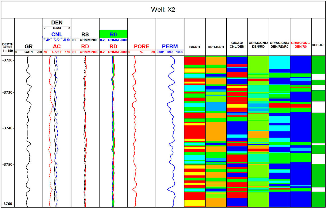
FIGURE 7. Comparison of automatic clustering division of logging facies with different parameter combinations.

Analysis of Logging Facies Division Results

The most important point of automatic clustering division of logging facies is the determination of input curve, which directly determines the accuracy of division results. Therefore, parameter optimization and comparative analysis of different parameter combinations are of particular importance. For the combination of different parameters of logging curves on the basis of the mechanism analysis, six groups of comparative experiments (Table 2) were carried out in this study, and six different parameter combinations were automatically clustered. The division results are shown in Figure 7. Based on the analysis of the division results of different parameter combinations, the basis for determining the best parameter combination for logging facies division mainly focuses on two basic principles: first, the division of reservoir and non-reservoir should be clear, that is, sandstone and mudstone can be clearly distinguished; second, the interface between reservoirs and non-reservoirs delineated by automatic clustering should be basically the same as the interface between reservoirs and non-reservoirs delineated by hand. According to the two basic principles, the division results of the six groups are analyzed as follows (Table 2):

TABLE 2

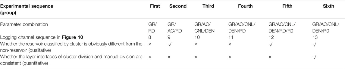
TABLE 2. Comparison of effects of automatic cluster division of logging facies with different parameter combinations.

The first group of parameter combinations is GR and RD (Channel 8 in Figure 7). GR and RD are the basic parameters for lithology and electrical identification in the “four property relationship,” respectively. The division results can generally reflect the distribution of reservoirs, but the reservoir division in some areas is not clear, and the sand mudstone cannot be clearly distinguished (green in Channel 8 in Figure 7 is actually mudstone, but green is distributed in the reservoir). Therefore, these two parameters alone cannot reflect the actual situation of the reservoir.

The second group of parameter combinations is GR, AC, and RD (Channel 9 in Figure 7). This group can give a better picture of the distribution of reservoir and non-reservoir. Sandstone and mudstone can be largely distinguished (except that the penultimate non-reservoir section is slightly unclear), but the thickness of the non-reservoir section (dark blue and light blue in Channel 9 in Figure 7 are mudstone) is relatively small, and the reservoir and non-reservoir interfaces divided by automatic clustering are not consistent with the reservoir and non-reservoir interfaces divided manually.

The third group of parameter combinations is GR, AC, CNL, and DEN (Channel 10 in Figure 7). The combination does not introduce resistivity parameters, so the division effect is very poor, and the division of the reservoir and non-reservoir is chaotic (red in Channel 10 in Figure 7 is distributed in both reservoir and non-reservoir sections), making it impossible to distinguish. Obviously, resistivity parameters are indispensable parameters for logging facies division.

The fourth group of parameter combinations is GR, AC, CNL, DEN, and RD (Channel 11 in Figure 7). The division results of this group of combinations can generally reflect the distribution of reservoirs, but the reservoir division in some areas is not clear and the sand mudstone cannot be clearly distinguished (the division of the first three reservoirs and non-reservoir sections in Channel 11 in Figure 7 is chaotic).

As discussed before (Resistivity Value of Saturated Pure Water R₀ section and Artificial Neural Network Prediction R₀ section), it is difficult to use formation resistivity to analyze the variability of actual formations as the resistivity values of low-permeability reservoirs are influenced by a variety of factors including physical properties, oil bearing properties, complex lithology, and pore structure.

Therefore, the resistivity R₀ saturated with pure water was introduced to remove the influence of physical property and rock property on resistivity (RD). Similarly, based on the combination of the first four parameters, the resistivity R₀ saturated with pure water was introduced for parameter combination to observe the division effect. The fifth group of parameter combinations is GR, AC, CNL, DEN, RD, and R₀ (Channel 12 of Figure 7). This group can better reflect the distribution of reservoir and non-reservoir, and the sandstone and mudstone can be basically distinguished (except that the second non-reservoir section and the third reservoir section are slightly unclear), but the thickness of the non-reservoir section (green and red in Channel 12 of Figure 7 are mudstone) is too large, and the reservoir and non-reservoir interfaces divided by automatic clustering are not consistent with the reservoir and non-reservoir interfaces divided manually.

The sixth group of parameter combinations is GR, AC, CNL, DEN, and R₀ (Channel 13 in Figure 7). The division results of this group meet the two basic principles that the reservoir and non-reservoir division can be significantly distinguished from the automatic clustering division and the reservoir and non-reservoir interface should be basically the same as the manually divided reservoir and non-reservoir interface, with the best division results.

Based on the division results, the best parameter combination of GR, AC, CNL, DEN, and R₀ logging facies was optimized. The division of logging facies provided an experimental and theoretical basis for further identifying the petrophysical facies of low-permeability reservoirs in this area.

The Supervised Identification of Petrophysical Facies

Pore Structure Classification

The reservoir pore structure facies refers to the geometry, size, distribution, and interconnection of pores and throats in rocks. It is a general term for the changes of pore structure in reservoir units. During the formation of a reservoir different diagenesis has a certain impact on the destruction and preservation of primary pores and the generation of secondary pores. The pore structure is the manifestation of the micro-impact on the reservoir.

According to the observation of core casting thin section, the dissolution of feldspar and rock debris in the Es₃ reservoir was developed; expanded intergranular pores, reduced intergranular pores, intragranular pores, and mold pores were also developed. There are many expanded intergranular pores, but the absolute content of pores is small, indicating that the intensity of dissolution is limited. According to the characteristics of diagenetic stage, diagenetic type, type of diagenetic minerals under microscope, formation sequence, strength of dissolution, and type and content of clay matrix, it can be divided into four diagenetic types: secondary solution pores, mica deformed by compaction, no obvious characteristics or transition, and carbonate cementation. Based on the data of different diagenetic types of core cast thin sections and the pore distribution of mercury injection test, the pore structure types of Es₃ reservoir in the study area were studied according to different pore structure parameters, and the reservoir pore structure facies were divided into four categories: I, II, III, and IV (Table 3).

TABLE 3

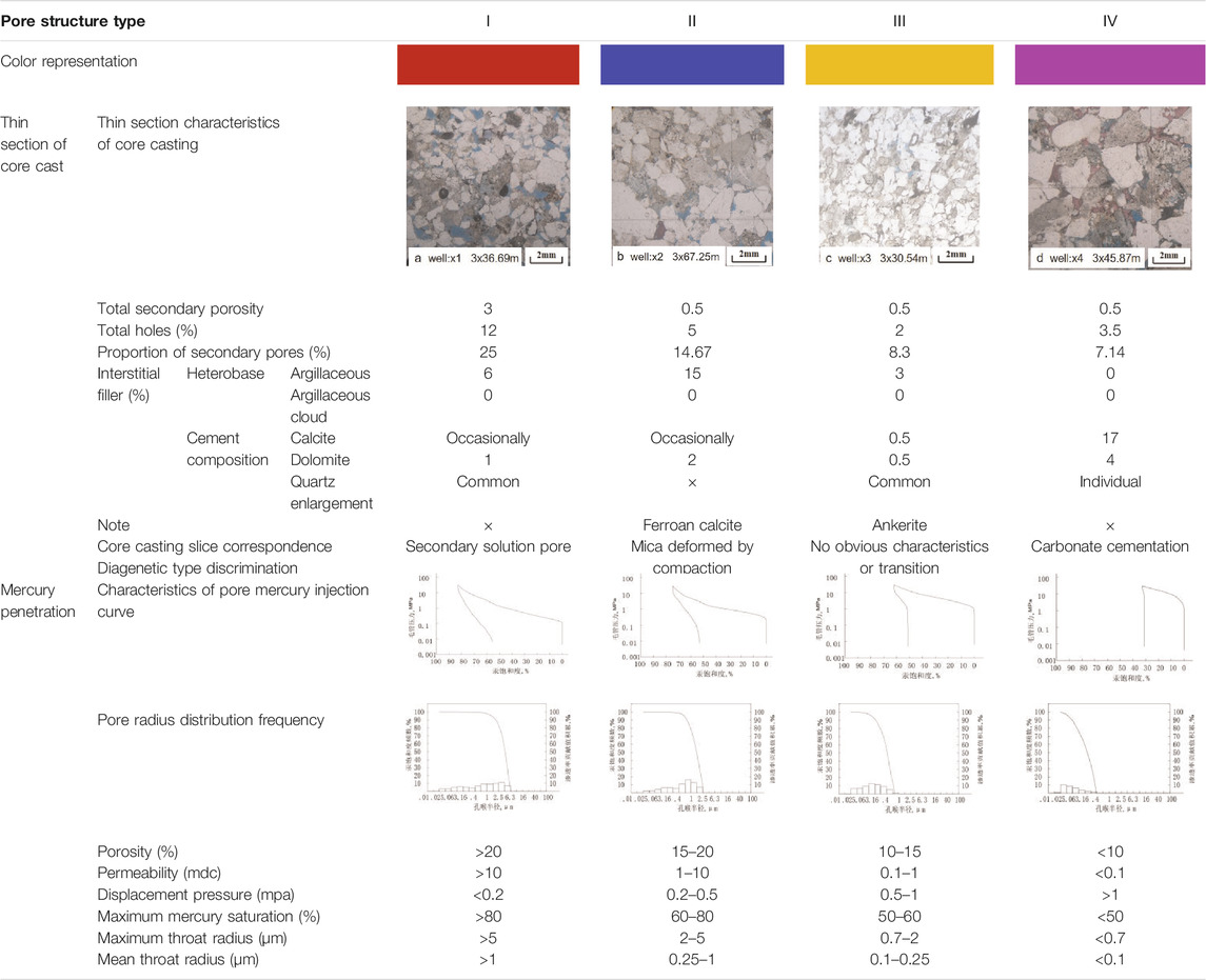
TABLE 3. Classification standard of pore structure of the Es₃ reservoir.

The diagenetic type of class I reservoir is mainly secondary solution pores, accounting for a relatively large proportion of secondary pores (the secondary pores of core cast thin section accounts for 25%), containing certain argillaceous matrix and obvious cements such as quartz and dolomite, with porosity greater than 15%, permeability greater than 10mdc, displacement pressure less than 0.2 MPa, maximum mercury saturation greater than 80%, and maximum throat radius greater than 5 μm. The mean throat radius is greater than 1.0 μm, and the throat is relatively large and well sorted, so it is a fine throat and is a good reservoir.

The diagenetic type of class II reservoir is mainly mica deformed by compaction, the proportion of secondary pores is slightly smaller than that of secondary solution pores, containing a large amount of argillaceous (the argillaceous content of core cast thin section b is 15), less cement, mostly iron calcite, porosity between 10 and 15%, permeability between 1 and 10 mdc, displacement pressure between 0.2 and 0.5 mpa, and maximum mercury saturation between 65 and 80%. The maximum throat radius is between 2 and 5 μm, and the mean throat radius is 0.25–1.0 μm, with fine throat and poor sorting; it is an ultra-fine throat and a medium reservoir.

The main characteristics of the diagenetic type of class III reservoirs are the absence of obvious features and transitions, a slightly higher proportion of secondary pores is slightly higher than that of carbonate cementation, a small amount of argillaceous matrix, quartz enlargement, dolomite, obvious calcite and other cements, mostly iron dolomite, porosity between 10 and 15%, permeability is between 0.1–1 mdc, displacement pressure is between 0.5 and 1 mpa, maximum mercury saturation is between 50 and 65%, maximum throat radius is between 0.7 and 2 μm, and mean throat radius is 0.1–0.25 μm, exceptionally fine pore throat, but good flow properties with moderately sorted and finely skew roar channel. It belongs to micro-throat and is a poor reservoir.

The diagenetic type of class IV reservoir is mainly carbonate cementation, and the proportion of secondary pores is the smallest among all diagenetic types shown in the figure (the secondary pores of core cast thin section D account for 7.14%), the content of matrix is small, the content of cement is large, and most of them are calcite, the content of calcite is 17%, the porosity is less than 10%, the permeability is less than 0.1 mdc, the displacement pressure is greater than 1.0 MPa, and the maximum mercury saturation is generally less than 50%, The maximum throat radius is less than 0.7 μm. The mean throat radius is less than 0.1 μm. It belongs to extra micro-throat, and this kind of reservoir is extra poor reservoir or ineffective reservoir.

Combination of Logging Facies and Identification of Petrophysical Facies

Considering diagenetic type, pore structure, and logging response characteristics, it is necessary to optimize and merge multiple logging facies obtained by automatic clustering. First, the logging facies considers the division of reservoir segments, and the quality of reservoir is closely related to the pore structure. By observing the pore and permeability range, mercury injection curve, pore radius, and diagenetic type of different logging facies, the logging facies with similar pore structure were combined as a whole. Second, the logging response characteristics should be considered, different logging response characteristics should be further optimized to merge and scale based on the combination of pore structure types, and finally the whole section can be divided into five types of logging facies; the combined logging facies were calibrated in combination with the petrophysical name obtained by core casting thin section analysis, making the corresponding logging facies to have petrophysical facies of geological characteristics (Song et al., 2013; Zhu, 2016). After combining, the five types of logging facies are named by petrophysics, and there are four types of sandstone petrophysical facies, including corrosion facies, argillaceous cementation facies, transition facies, calcarenite facies, and mudstone (in Table 4, Figures 8, 9; the 8th pore structures in Figure 9 are pore structure facies, and the color distribution corresponds to Table 3, where white is the non-reservoir section. The 9th petrophysical in the figure is petrophysical facies, and the color distribution corresponds to Table 4, in which white is the non-reservoir section):

TABLE 4

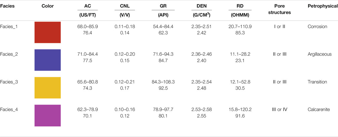
TABLE 4. Typical characteristics of different petrophysical facies in the Es₃ reservoir.

FIGURE 8

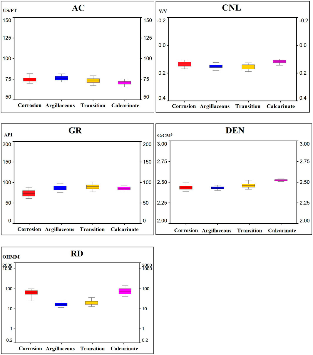
FIGURE 8. Logging response box diagram of different petrophysical facies in the Es₃ reservoir.

FIGURE 9

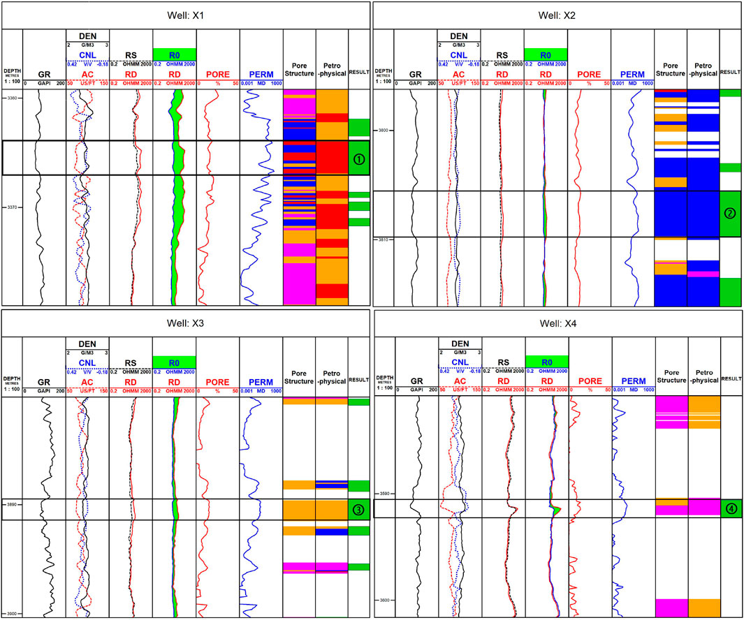
FIGURE 9. Results plot of different petrophysical facies of the Es₃ reservoir.

Facies_1 is corrosion facies with relatively good physical properties. The reservoir is a dominant reservoir with relatively high productivity (Figure 9 ①). The corresponding reservoir pore structure type is class I or class II (Table 3, Channel 8 of Figure 9). The logging response is characterized by the “three low, one medium, and one high” of low DEN, CNL, and GR values; medium AC value; and high RD value. The distribution range of AC value is 68.0–85.9 us/ft, the distribution range of CNL value is 0.11–0.18 V/V, the distribution range of GR value is 54.4–84.4 API, the distribution range of DEN value is 2.35–2.51 g/cm³, and the distribution range of RD value is 20.7–110.9 Ω m.

Facies_2 is argillaceous cementation facies with relatively general physical properties. The reservoir is a medium reservoir with low productivity (Figure 9 ②). The corresponding reservoir pore structure type is class II or class III. The logging response has the characteristics of “three low and two medium” of low CNL, DEN, and RD values; medium AC and GR values. The distribution range of AC value is 71.0–84.4 us/ft, and the distribution range of CNL value is 0.12–0.20 V/V. The distribution range of GR value is 71.6–94.3 API, the distribution range of DEN value is 2.36–2.46 g/cm³, and the distribution range of RD value is 11.1–28.2 Ω m.

Facies_3 is transition facies with poor physical properties. The reservoir is a poor reservoir with low productivity (Figure 9 ③). The corresponding reservoir pore structure type is class III or class IV, and the logging response is characterized by “one low, two medium, and two high” of low RD value, medium DEN and AC values, and high CNL and GR values. The distribution range of AC value is 65.6–80.8 us/ft, and the distribution range of CNL value is 0.12–0.21 V/V. The distribution range of GR value is 84.3–108.3 API, the distribution range of DEN value is 2.35–2.54 g/cm³, and the distribution range of RD value is 12.1–52.8 Ω m.

Facies_4 is calcarenite facies with extremely poor physical properties. The reservoir is an extremely poor reservoir with extremely low productivity (Figure 9 ④). The corresponding reservoir pore structure type is class III or class IV. The logging response is characterized by the “three low and two high” of low AC, CNL, and GR values and high DEN and RD values. The distribution range of AC value is 62.3–78.9 us/ft, and the distribution range of CNL value is 0.10–0.16 V/V, the distribution range of GR value is 78.9–97.7 API, the distribution range of DEN value is 2.53–2.58 g/cm³, and the distribution range of RD value is 15.8–120.2 Ω m.

Based on the previous results, the corresponding relationship between logging facies combination and petrophysical facies identification was well explained, and the accuracy of logging facies division and petrophysical facies identification of low-permeability sandstone reservoir in this study was fully verified.

Physical Property Relationship and “Sweet Spot” Evaluation of Different Rock Petrophysical Facies

Using the rock petrophysical facies analysis method to classify and evaluate reservoirs can fully consider the main geological factors affecting characteristics of the reservoir micropore structure. These factors are finally reflected in the differences of reservoir porosity and permeability (Cui, 2015) (Figure 10). The corrosion facies is the dominant facies belt, and the physical properties of the reservoir in which this kind of petrophysical facies is developed are the best. Secondary pores account for a large proportion of the pore space. The pore types are mainly residual primary intergranular pores and secondary dissolution pores. The pore throat connectivity is good, the pore permeability value is relatively high, with porosity generally greater than 15%, and the permeability is greater than 10 mdc. The calcarenite facies is mainly affected by the cementation of carbonate rocks in the diagenetic stage, and its physical properties are poor. Although it has undergone corrosion transformation at a later stage, it cannot change the fact that its physical properties are poor. Among the four petrophysical facies, the calcarenite facies has the lowest porosity and permeability, most less than 10%, the permeability is less than 0.1 mdc, with a relatively high slope of porosity and permeability, R² = 0.7771. The argillaceous cemented facies is mainly affected by the deformation of mica by compaction. Its reservoir physical properties are between the corrosion facies and the transition facies (or calcarenite facies). Although it is also in the dominant facies belt, it has experienced complex diagenesis, the pore structure is relatively complex, reservoir heterogeneity is obvious, and its pore permeability characteristics show a low slope relationship. The transitional facies is mainly affected by the dissolution of unstable components, clay rim cementation, secondary increase of quartz or strong compaction, and protogenetic rock. Although it has undergone certain diagenetic transformation at a later stage, it still cannot change the characteristics of relatively poor reservoir physical properties. Similar to the calcarenite facies, its porosity and permeability value is also low, with permeability almost less than 1 md.

FIGURE 10

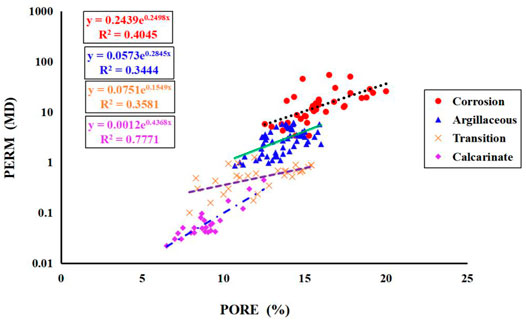
FIGURE 10. Relationship between porosity and permeability of different petrophysical facies in the Es₃ reservoir.

Studies have found that the desserts of low-permeability sandstone reservoirs are mostly concentrated in the secondary pores with large primary porosity or local corrosion development. Represented by corrosion facies, the pore structure is good and the productivity is high. The total production of oil layer represented by layer ① is as high as 106 m³ (Figure 11 shows the distribution range of PORE and PERM values of different petrophysical facies and the productivity of different petrophysical facies represented by four sub-layers). Due to the high mud volume and obvious heterogeneity of the argillaceous cemented facies, there is a big gap between the productivity and the corrosion facies. The total production of the oil layer represented by layer ② is 14.52 m³. Due to the “calcium content,” the resistivity of calcarenite facies is high but affected by the cementation of carbonate rock, and the physical property is very poor and the productivity is very low. The total output represented by layer ④ is only 0.83 m³. The transitional facies has a complex composition, poor pore structure, and physical properties between argillaceous cemented facies and calcarenite facies, with low production capacity. The total production of oil layer represented by layer ③ is only 3.25 m³. By comparing the huge differences in productivity of different petrophysical facies, it is of great significance to predict the “sweet spot” of low-permeability sandstone reservoir and adjust oilfield development measures. Generally speaking, perforation development is preferred for “sweet spot” of low permeability, while fracturing is an efficient stimulation measure to improve production. Different methods can be used for fracturing measures of reservoirs with different petrophysical facies. For calcarenite facies and transition facies with low production capacity, due to the metasomatic filling of carbonate minerals, the primary pores are destroyed. During fracturing, acid fracturing fluid should be properly used to transform the reservoir to improve production.

FIGURE 11

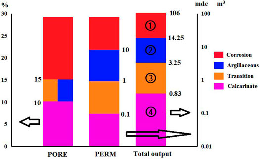
FIGURE 11. Comparison of porosity and permeability distribution and productivity of different petrophysical facies in the Es₃ reservoir. (Note: Total output is the production, ① ②, ③, and ④, respectively, correspond to the four sub-layers in Figure 9; pore is the main coordinate axis, and its unit is %; PERM and total output are secondary coordinate axes, and the units are mdi and m³, respectively.)

Conclusion

In this study, a semi-supervised learning model based on petrophysical facies delineation was modeled using conventional logging data, combined with mercury injection data and core cast thin layers, which improved the efficiency and accuracy of petrophysical facies division, and greatly improved the accuracy of “sweet spot” identification, so as to solve the problem in that it is difficult to predict the dominant section of low-permeability sandstone reservoir and better grasp the productivity of reservoir. The reservoir heterogeneity characterization based on petrophysical facies transformed the heterogeneity problem into a homogenization problem, realized the classified evaluation of reservoir macro-physical properties and the micropore structure, improved the accuracy of reservoir characterization, and provided a basis for reservoir evaluation and prediction of dominant facies to find “sweet spot area.”

1) There are many classification methods for low-permeability sandstone reservoirs, but they have limitations in varying degrees. The petrophysical facies can provide a comprehensive characterization of the pore structure and genesis of rocks and better reflects differences in productivity. Therefore, this classification method has great advantages. The automatic clustering (MRGC) algorithm divides logging facies by calculating nearest neighbor index NI and uses kernel representative index (KRI) to determine the best number of logging facies, making it an ideal method for logging facies division of low-permeability sandstone reservoir.

2) The artificial neural network was used to predict the resistivity R₀ saturated with pure water to remove the influence of lithology and physical properties on the resistivity, and the superposition of resistivity R₀ saturated with pure water and deep lateral resistivity was consistent with the actual results, providing a theoretical basis for the identification of “sweet spot” of low-permeability reservoirs with a complex pore structure.

3) In this study, a semi-supervised learning was used to divide petrophysical facies and “sweet spot” identification. Unsupervised clustering and supervised recognition were well combined. This “unsupervised/supervised” or semi-supervised learning model was extended to the whole region training prediction for “sweet spot” identification. Experimental results showed that the prediction results of the model were in good agreement with the actual results; from the observation of core cast thin section to logging modeling and from diagenetic characteristics to determination of petrophysical facies division, this scaling evaluation problem from the millimeter level to meter level has been applied well in this study.

4) Through the analysis of the physical property relations of different petrophysical facies, the porosity and permeability of different petrophysical facies have different slope relations and they vary widely, which provides a certain theoretical basis for the subsequent better study of the physical property relations and “sweet spot” identification of low-permeability sandstone reservoirs. It is of great significance for predicting the “sweet spot” of low-permeability sandstone reservoir and adjusting oilfield development measures. In general, perforation development is preferred for “sweet spot” of low-permeability, and fracturing is an efficient stimulus to improve production.

Data Availability Statement

The original contributions presented in the study are included in the article/Supplementary Material; further inquiries can be directed to the corresponding author.

Author Contributions

All authors listed have made a substantial, direct, and intellectual contribution to the work and approved it for publication.

Conflict of Interest

Author HF and XL were employed by the company China National Offshore Oil Corporation.

The remaining authors declare that the research was conducted in the absence of any commercial or financial relationships that could be construed as a potential conflict of interest.

Publisher’s Note

All claims expressed in this article are solely those of the authors and do not necessarily represent those of their affiliated organizations, or those of the publisher, the editors, and the reviewers. Any product that may be evaluated in this article, or claim that may be made by its manufacturer, is not guaranteed or endorsed by the publisher.

References

Chai, Y., and Wang, G. (2016). Petrophysical Facies Classification and Prediction of High Quality Tight sandstone Reservoirs: A Case Study of the Second Member of Xujiahe Formation in Anyue Area, central Sichuan Basin[J]. Lithologic Reservoirs (3), 74–85. doi:10.3969/j.issn.1673-8926.2016.03.011

CrossRef Full Text | Google Scholar

Cui, L. (2015). Logging Interpretation Based on Petrophysical Facies: A Case Study of Chang 7 Reservoir in Huanjiang Oilfield, Xian: Xi’an Shiyou University[D].

Google Scholar

Fang, M., Zeng, X., and Liang, D. (2011). “Application of Artificial Neural Network in Grain Size Prediction of Reservoir[C],” in Proceedings of the International Conference on Oil and Gas Reservoir Monitoring and Management, Xi’an, Shaanxi, China, October 20, 2011.

Google Scholar

Gan, C. (1994). Une approche de classification non supervisee base sur la Đotion desk plus proches voisins[D]. France: University of Technology of Compiegne.

Google Scholar

Gong, L., Fu, X., Wang, Z., Gao, S., Jabbari, H., Yue, W., et al. (2019). A New Approach for Characterization and Prediction of Natural Fracture Occurrence in Tight Oil Sandstones with Intense Anisotropy. Bulletin 103 (6), 1383–1400. doi:10.1306/12131818054

CrossRef Full Text | Google Scholar

Gong, L., Wang, J., Gao, S., Fu, X., Liu, B., Miao, F., et al. (2021). Characterization, Controlling Factors and Evolution of Fracture Effectiveness in Shale Oil Reservoirs. J. Pet. Sci. Eng. 203, 11. doi:10.1016/j.petrol.2021.108655

CrossRef Full Text | Google Scholar

Grana, D., Pirrone, M., and Mukerji, T. (2012). Quantitative Log Interpretation and Uncertainty Propagation of Petrophysical Properties and Facies Classification from Rock-Physics Modeling and Formation Evaluation Analysis[J]. Geophysics 77 (3), 45. doi:10.1190/geo2011-0272.1

CrossRef Full Text | Google Scholar

Guo, R., and Gao, P. (1996). “Application of Artificial Neural Network (ANN) in Logging Reservoir Evaluation[C],” in Proceedings of the 12th Annual Conference of Chinese Geophysical Society, Xi’an, Shaanxi, China, October 1996.

Google Scholar

Huang, Y., Wan, J., and Sun, P. (2017). Comprehensive Logging Evaluation of Complex Reservoir Based on Petrophysical Facies Analysis[J]. J. Yangtze University 14 (1), 32–39.

Google Scholar

Jin, L., Wang, G., and Chen, M. (2013). Classification and Evaluation of Reservoir Pore Structure Based on Petrophysical Facies: A Case Study of Chang 8 Oil Formation in Jiyuan Area, Ordos Basin[J]. Pet. Explor. Develop. 40 (5), 000566–000573. doi:10.11698/PED.2013.05.08

CrossRef Full Text | Google Scholar

Jin, L., Wang, G., and Wang, S. (2013). Review and Research Progress of Logging Identification Methods for Diagenetic Facies in Clastic Reservoirs[J]. J. Cent. South Univ. 44 (12), 4942–4953.

Google Scholar

Jin, L., Wang, G., and Huang, L. (2015). Quantitative Division of Diagenetic Facies of Tight sandstone Reservoir and its Logging Identification Method[J]. Bull. Mineral. Petrol. Geochem. 34 (1), 128–138.

Google Scholar

Lai, J. (2016). Logging Quantitative Characterization Method and Application of Tight Reservoir Petrophysical Facies in Kuqa Depression, Beijing: China University of Petroleum.

Leite, V. C., Silva, P. M. C., Gattass, M., and Silva, A. (2013). “Analysis of Ensemble Methods Applied to Lithology Classification from Well Logs[C],” in 13th International Congress of the Brazilian Geophysical Society & EXPOGEF, 26-29 August, 2013, 𝐑io de Janeiro, Brazil (Society of Exploration Geophysicists and Brazilian Geophysical Society), 949–952.

Google Scholar

Li, X., and Li, H. (2013). A New Method of Identification of Complex Lithologies and Reservoirs: Task-Driven Data Mining. J. Pet. Sci. Eng. 109, 241–249. doi:10.1016/j.petrol.2013.08.049

CrossRef Full Text | Google Scholar

Li, Q., and Ying, Li. (2012). Synthetic R₀ Technique Used to Identify Oil and Water Layers[J]. Sci. Techn. Eng. 012 (15), 3738–3740.

Google Scholar

Lifei, B., Li, Z., and Liu, H. (2021). Research on Semi-supervised Learning Algorithm for Lithology Prediction Based on Label Propagation. Prog. Geophys. 36 (2), 0540–0548. doi:10.6038/pg2021EE0181

CrossRef Full Text | Google Scholar

Lu, P., and Liu, L. (2012). Lithology Identification Method of Conglomerate Reservoir Based on Rock Physical Facies[J]. Oil-Gasfield Surf. Eng. 31(07), 90. doi:10.3969/j.issn.1006-6896.2012.7.057

CrossRef Full Text | Google Scholar

Shi, Y., Zhang, H., and Hou, Y. (2005). Fine Interpretation Modeling of Logging Reservoir Parameters Based on Petrophysical Facies Classification[J]. Well Logging Techn. 29 (4), 328–332. doi:10.3969/j.issn.1004-1338.2005.04.014

CrossRef Full Text | Google Scholar

Shi, X., Cui, Y., Guo, X., Yang, H., Chen, R., Li, T., et al. (2017). “Logging Facies Classification and Permeability Evaluation: Multi-Resolution Graph Based Clustering[C],” in SPE Technical Conference & Exhibition San Antonio, TX, USA, October 09, 2017. doi:10.2118/187030-MS

CrossRef Full Text | Google Scholar

Shi, X., Lv, H., and Cui, Y. (2018). Logging Phase Division and Permeability Evaluation Based on Graph Theory Multi-Resolution Clustering Method: A Case Study of Guantao Formation, W Well Block, P Oilfield, Bohai Sea[J]. China Offshore Oil and Gas 030 (1), 81–88. doi:10.11935/j.issn.1673-1506.2018.01.010

CrossRef Full Text | Google Scholar

Soete, J., Huysmans, M., and Claes, H. (2014). Petrophysical and Geostatistical Analysis of Porosity-Permeability and Occurrence of Facies Types in continental Carbonates of the Ballık Area. Denizli, Turkey: The Geological Society.

Google Scholar

Song, Q., Zhang, Z., and Zhang, C. (2013). Application of Logging Facies - Lithofacies Analysis Technique in Complex Lithology[J]. J. Oil Gas Techn. 35 (7), 78–81. doi:10.3969/j.issn.1000-9752.2013.07.017

CrossRef Full Text | Google Scholar

Sun, P. (2016). Petrophysical Model and Heterogeneity Characterization of Donghe sandstone Reservoir Based on Donghe 1 oilfield[D]. Beijing: China University of Petroleum.

Google Scholar

Tian, Y., Xu, H., Zhang, X.-Y., Wang, H.-J., Guo, T.-C., Zhang, L.-J., et al. (2016). Multi-resolution Graph-Based Clustering Analysis for Lithofacies Identification from Well Log Data: Case Study of Intraplatform Bank Gas fields, Amu Darya Basin. Appl. Geophys. 13 (4), 598–607. doi:10.1007/s11770-016-0588-3

CrossRef Full Text | Google Scholar

Wang, B. (2018). Petrophysical Facies Classification and Favorable Area Prediction of Low Permeability sandstone reservoir[D]. Xian: Northwest University.

Wei, J., Yang, B., and Liu, F. (2020). BP Neural Network Porosity Prediction Based on Lithology Identification[J]. Petrochem. Industry Appl. 39, 111–116.

Google Scholar

Wu, H., Wang, C., Zhou, F., Yuan, Y., Wang, H. F., and Xu, B. S. (2020). An Adaptive Multi-Resolution Graph Clustering Method for Logging Phase Analysis[J]. Appl. Geophys. 17, 13–25. doi:10.1007/s11770-020-0806-x

CrossRef Full Text | Google Scholar

Yao, G., Zhao, Y., and Zhang, S. (1995). Petrophysical Facies of Low Permeability and Fine Grain Reservoir Sandstones in Xinmin Oilfield[J]. Earth Sci. 355–360.

Google Scholar

Ye, S., and Rabiller, P. (2000). “A New Tool for Electro-Facies Analysis : Graph-Based Clustering[J],” in SPWLA Annual Logging Symposium.

Google Scholar

Zhang, M. (2018). Research on Multi - Level Self - Organization and Automatic Classification of Stratum lithology[D]. Wuhan: Yangtze University Dallas, TX, USA, June 04, 2017.

Zhu, P. (2016). Logging Evaluation Method of Low Permeability sandstone Reservoir and its application, Qingdao: China University of Petroleum, East China[D].