Mangrove Growth Monitoring Based on Camera Visible Images—A Case Study on Typical Mangroves in Guangxi

Mangroves are an important coastal wetland ecosystem, and the high-throughput visible light (RGB) images of the canopy obtained by the ecological meteorological station can provide basic data for quantitative and continuous growth monitoring of mangroves. However, as for the mangroves that are subject to periodic seawater submersion, some key technical issues such as image selection, vegetation segmentation, and index applicability remain unsolved. With the typical mangroves in Beihai, Guangxi, as the object in this study, we used canopy RGB images and tidal data to find out the screening methods for high-quality nontidal submerged images, as well as the vegetation segmentation algorithms and RGB vegetation index applicability, so as to provide technical reference for the use of RGB images to monitor mangrove growth. The results showed that: 1) The critical tide levels can be determined according to the periodic changes of submersion in the mangroves, and critical tidal levels and image brightness can be used to quickly screen high-quality images of mangroves that are not submerged by seawater. 2) Machine learning and NLM filtering are effective strategies to obtain high-precision mangrove segmentation results. The machine learning algorithm has superiority in the segmentation of mangrove vegetation with a segmentation accuracy of higher than 80%, and the nonlocal mean filtering can effectively optimize the segmentation results of various algorithms. 3) The seasonal index VEG and antiseasonal index CIVE can be used as the optimal indices for mangrove growth monitoring, and the compound sine function can better simulate the change trend of various RGB vegetation indices, which is convenient for quickly judging mangrove growth changes. 4) Mangrove RGB vegetation indices are sensitive to meteorological factors and can be used to analyze the influence of meteorological conditions on mangrove growth.

1 Introduction

As a special ecosystem at the land–sea interface, mangroves encompass both important ecological service functions and socioeconomic values (Zhu et al., 2014). It can play an important role in wind and wave defense, pollution prevention, and beautification of the coast. Quantitative monitoring of mangrove growth conditions can provide an important data basis for in-depth interpretation of mangrove ecosystem functions. As the mangroves that grow on the intertidal zone of the coast or at the mouth of the river are subject to periodic tidal submersion (Zhang and Zheng, 1997), there are some problems in the traditional field sampling growth survey, such as lack of representativeness, and it is difficult for investigators to enter the mangrove growth area (Wen et al., 2020). Satellite remote sensing technology provides a convenient means for mangrove growth monitoring. The leaf area index (Ramsy and Jensen, 1996; Kovacs et al., 2005) and normalized vegetation index (Cao, 2017) retrieved by remote sensing can be used for mangrove health monitoring. However, due to the satellite revisit cycle and cloud and rain weather, it is difficult to ensure the continuity of high-resolution satellite remote sensing data suitable for mangrove growth monitoring (Zhang, 2016; Zhu et al., 2020). Thus, both traditional ground survey and satellite remote sensing technology have some problems, such as lack and incompleteness of key information, which is difficult to be used for quantitative and continuous monitoring of mangrove growth.

In recent years, the widespread construction of ecological meteorological observatories in China has made camera visible light (RGB) images become normalized data. As an important part of the space–air–ground integrated monitoring network, this type of data can be an effective supplement to satellite remote sensing and UAV remote sensing, making it able to achieve the high-throughput time-series monitoring of vegetation growth. Guangxi established a mangrove ecological meteorological observation station in 2018, providing important basic data for mangrove growth monitoring. However, the current key technologies of RGB images are mainly applied to crops, and it has been proven that the technologies can effectively monitor the growth period (Lu et al., 2011; Wu, 2014; Wu et al., 2018; Liu et al., 2020), coverage (Purcell, 2000; Campillo et al., 2008; Yang et al., 2018), growth vigor (Zhou et al., 2015; Han et al., 2019), and nitrogen status (Chen et al., 2017; Shi et al., 2020) of crops. Although UAV RGB images have achieved initial success in mangrove vegetation segmentation and canopy structure inversion (Jones et al., 2020; Wen et al., 2020), whether the RGB images acquired by the ground are effective in monitoring mangrove growth conditions remains to be clarified. Moreover, some key issues related with image selection, vegetation segmentation, and index applicability for mangroves, which are subject to periodic seawater submersion, are still rarely reported.

Image selection is the primary problem to be solved to apply RGB images in mangrove monitoring. Mostly shot in fixed time and fixed angle in the station, the canopy images can be obtained at multiple times in a day. Long-term sequence monitoring involves the screening of a large number of image data. Therefore, for mangroves, first of all, it is necessary to ensure that the selected images are not affected by seawater submersion. Under the effect of tides, the rise and fall of seawater change, and the submerging time of mangroves in different regions is also different (Zhang and Zheng, 1997), which brings difficulties to the selection of mangrove canopy images. In addition, the quality of the obtained canopy image will be different due to the influence of light conditions. Therefore, the selection of mangrove canopy images involves two issues: analysis of tidal submerging rules and judgment of image brightness.

Vegetation segmentation is a key technology in using RGB images to carry out mangrove monitoring. Image segmentation aims to divide the images containing the spatial distribution information of complex surface features into different regions with specific semantic labels (Min et al., 2020), which is the basis for vegetation monitoring using near-ground canopy RGB images. Currently, the developed segmentation methods include area (Liu et al., 2021), histogram thresholding (Chen et al., 2011), feature space clustering (Li et al., 2020), edge detection (Ren et al., 2004), fuzzy technology (Ma et al., 2008), artificial neural network (Ma et al., 2020), and deep learning (Yan et al., 2021). At present, these segmentation algorithms have been successfully applied in crops, but there has been no report on the application in mangroves.

The selection of monitoring index is the basis for the quantitative monitoring and evaluation of mangrove growth. At present, scholars have constructed various RGB vegetation indices to monitor the changes in crop growth, namely, NDYI (normalized difference yellowness index) (Sulik and Long, 2016), GLA (green leaf algorithm) (Guijarro et al., 2011), VARI (visible atmospherically resistant index) (Gitelson et al., 2002), and NGRDI (normalized green-red difference index) (Pérez et al., 2000). However, due to the wavebands and parameter composition, the developed indices are mostly for crops, and the applicability of these indices in mangrove growth monitoring also needs to be reassessed.

The objective of this study was to demonstrate the plausibility of monitoring and evaluating the canopy growth of mangrove using the existing RGB image processing technology. To achieve this objective, we performed the analysis on the screening method of high-quality nontidal submerging images, developed the high-precision segmentation algorithm of mangrove vegetation, and applied RGB image-based vegetation indices to monitor mangrove growth. This study provides technical references for the application of RGB images in the rapid and accurate monitoring of mangrove growth.

2 Data and methods

2.1 Study area

Completed at the end of 2018, the Beihai Mangrove Ecological Meteorological Observatory is located in the small bay (21°27′5.57″N, 109°18′4.39″E) of the National Marine Science and Technology Park in Beihai City, Guangxi. The geographical location is shown in Figure 1. The study area has a subtropical monsoon climate, warm and humid throughout the year, with an average annual rainfall of 1,644.0 mm and an average annual temperature of 22.6°C. The mangrove forest in the study area has a total area of about 5.5 hm², where the species is dominated by the Aricennia marina community, mixed with some Kandelia obovata and Aegiceras corniculata. The soil is mainly composed of fine gravel sand to coarse sand, which has low organic matter content.

FIGURE 1

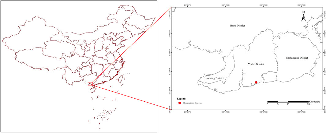
FIGURE 1. The geographical location of the ecological observatory.

2.2 Data

2.2.1 RGB images

The RGB images were taken from the digital camera erected on the flux tower of the ecological meteorological observatory. The camera was erected at 6 m above the ground. The camera model is ZQZ-TIM, and it uses a 1/1.8 inch CMOS sensor with the total pixels of about 6.44 million, aperture value of F1.5-4.3, 30 times optical zoom, 16 times digital zoom, wide dynamic effect, plus image noise reduction function, all of which enable it to better display day/night images. Moreover, the camera can achieve continuous monitoring with 360° continuous rotation in the horizontal direction, continuous monitoring after −20°–90° autoflip to 180° in the vertical direction, which has no blind spot monitoring. After acquisition, the images can be uploaded to the cloud platform or imported into the computer for processing. The RGB images were collected from 8:00 to 17:00 every day, with an interval of 1 h, and the image sequence time period was from September 3, 2018 to August 31, 2019.

2.2.2 Meteorological and tidal data

The meteorological data was collected from the automatic meteorological observation equipment of the ecological meteorological observatory. The observation elements included daily average temperature, daily maximum temperature, daily minimum temperature, relative humidity, and precipitation. The tidal data came from the Chinese Tide Table (Beihai port) compiled by the China Oceanic Information Center, and the observation elements included the tidal levels in every hour, time of tide, and tidal levels. These data were combined with RGB images to analyze the critical tidal levels when mangroves were submerged in seawater.

2.3 Research methods

2.3.1 RGB image selection

Image selection is to reduce the impact of tidal submersion, cloud covering, and illumination changes on the image quality of mangrove canopy, so as to obtain better images for vegetation segmentation and index calculation. First, the critical tidal level of seawater submersion in the study area was determined through the combination of visual interpretation and tidal data. Then the visual images with lower tidal levels were screened out. Finally, the image with the highest brightness was selected as the image of the day. During the process, the brightness of the visible images was represented by the sum of the R, G, and B color channel values (Peter et al., 2018). The critical tidal levels of the mangroves in the study area were determined as follows: 1) Randomly select the visible image data set with seawater submersion for 3 days every month. 2) Find the images with a small amount of water or completely exposed mud flat after comparing the submerging status in the mud flat on the images, and use the shooting time of the image as the time when the tide begins to rise or finishes falling. 3) Determine the critical tidal level according to the tide table at that time.

2.3.2 RGB image segmentation

The purpose of image segmentation is to accurately obtain green vegetation information from the entire image. In order to find a better segmentation algorithm for mangrove vegetation, we compared the accuracy of three different types of segmentation algorithms. The first algorithm used the individual channel of color space as the input of the Ostu threshold segmentation algorithm (Ostu, 1979) to achieve the automatic segmentation of vegetation. For example, there is a significant difference in the S channel in HSV space and in a channel in lab space between vegetation and background in RGB images, and values of these two channels both showed bimodal distribution in the image, providing the basis of automatic segmentation. The second used the nonlinear calculation by combining values of different channels, which enhanced proportion of green components and showed significant difference and pattern between vegetation and background in RGB images. A widely used and proven color index ExG was applied to discriminate vegetation from non-vegetation part in this study. The third segmentation algorithm that is based on machine learning took advantage of training classifiers with multidimensional classification samples to utilize rich information by mapping indistinguishable problems at low dimension to a high dimension. The K-means unsupervised clustering was first performed to generate training samples that were divided into vegetation, dark background, and bright background. Then features of vegetation pixels including 24 indexes from the dimension of color, texture, and gradient were extracted from the training samples to generate classification feature vectors. The support vector machine (SVM) was then used to classify vegetation and background in images.

Affected by factors such as differences in lighting conditions and imaging quality, it is fairly probable for the marginal part of vegetation to be wrongly segmented. In order to reduce the erroneous segmentation of leaf edges, nonlocal means (NLM) was introduced to optimize the results of vegetation segmentation. The NLM operator can protect the long and narrow structure similar to the vegetation leaf, and eliminate the ambiguity of pixel segmentation at the edge of the vegetation leaf by enhancing the nonadjacent pixels on the same structure within a certain neighborhood. The principle of the NLM algorithm is as follows:

Assume that the noising image is $v=\left\{v\left(a\right)|a\in A\right\}$, the image after denoising is $NL\left[v\right]$, then the weighted value of each pixel a can be calculated by the following formula:

$NL\left[v\right]\left(\mathrm{a}\right)=\frac{1}{\text{C}\left(\mathrm{a}\right)}{\displaystyle \sum }_{\text{b}\in \text{I}}w\left(a,b\right)v\left(b\right)$

where $w\left(a,b\right)$, is the weight of the similarity between pixel a and pixel b (Gaussian weighted Euclidean distance), which meets the requirement of $0\le w\left(a,b\right)\le 1$ and ${\displaystyle {\sum }_{b}w\left(a,b\right)=10\le \le 1}$. The formula is as follows:

$w\left(\mathrm{a},b\right)=\frac{1}{\text{C}\left(\mathrm{a}\right)}\text{exp}\left(-\frac{\Vert v\left(N\left(a\right)\right)-v{\left(N\left(b\right)\right)\Vert }_{2,\text{a}}^2}{h^2}\right)$

$C\left(\mathrm{a}\right)={\displaystyle \sum }_{\text{b}\in \text{I}}exp\left(-\frac{\Vert v\left(N\left(a\right)\right)-v{\left(N\left(b\right)\right)\Vert }_{2,\text{a}}^2}{h^2}\right)$

where ${\Vert v\left(N\left(a\right)\right)-v\left(N\left(b\right)\right)\Vert }_2^2$ is the square of the Gaussian weighted distance between the pixel in the subblock centered on pixel a and the pixel in the subblock centered on pixel b, which is used to measure the similarity between two pixels; a is the standard deviation, $v\left(N\left(a\right)\right)$ is the set of local sub-block pixels around a; and h is the filter parameter.

The onsite labeling results were used as reference to evaluate the accuracy of the classified images obtained before and after the filtering of the above three segmentation algorithms. The accuracy evaluation indicators Qseg and Sr are calculated as follows:

$Q_{\text{seg}}=\frac{{\displaystyle {\sum }_{i=0}^{i=m}{\displaystyle {\sum }_{j=0}^{j=n}\left(A{\left(p\right)}_{ij}\cap B{\left(p\right)}_{ij}\right)}}}{{\displaystyle {\sum }_{i=0}^{i=m}{\displaystyle {\sum }_{j=0}^{j=n}\left(A{\left(p\right)}_{ij}\cup B{\left(p\right)}_{ij}\right)}}}$

$S_{\text{r}}=\frac{{\displaystyle {\sum }_{i=0}^{i=m}{\displaystyle {\sum }_{j=0}^{j=n}\left(A{\left(p\right)}_{ij}\cap B{\left(p\right)}_{ij}\right)}}}{{\displaystyle {\sum }_{i=0}^{i=m}{\displaystyle {\sum }_{j=0}^{j=n}B{\left(p\right)}_{ij}}}}$

where, A is the foreground (green vegetation) pixel set (p = 255) or background (information other than green vegetation) pixel set (p = 0) of the segmented image, B is the foreground pixel set obtained by field labeling (p = 255) or background pixel set (p = 0), m and n are the number of lines and columns of the image, respectively, and i and j are the corresponding coordinates, respectively. The larger the Qseg and Sr values indicate higher segmentation accuracy. Qseg is the overall consistency of the background and foreground segmentation results, while Sr only represents the consistency of the foreground segmentation result.

2.3.3 Calculation and simulation RGB vegetation indices

The calculation of RGB vegetation indices is as follows: After the segmentation of the green vegetation in the visible image, the R, G, and B color channel values of each pixel in the green vegetation area were extracted, then all the pixels in the area were averaged, and finally, the visible vegetation indices of mangroves were calculated (Table 1).

TABLE 1

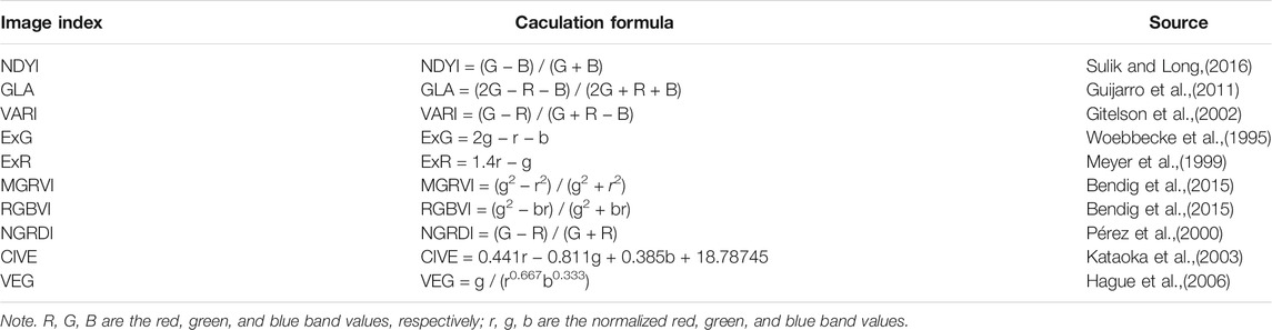
TABLE 1. RGB vegetation indices.

Vegetation change trend was simulated as follows: the compound sine function was used to simulate the change trend of mangrove growth over time, which was mainly used for quick judgment of mangrove growth. The calculation formula is as follows:

$VI=a+b\sin \left[\frac{2\pi \left(t_{day}-c\right)}{365}\right]$

where, a, b, and c are all empirical coefficients, and t_day is the day order.

The change rules of the various indices and the simulation results of vegetation change trend were compared to analyze the applicability of RGB vegetation indices for mangrove monitoring.

3 Result analysis

3.1 Fast screening of mangrove images

Affected by the tidal force of different cycles and the topography of the coastal zone, the tidal levels of the sea area presented a complex periodic movement over time. According to the submerging degrees classified by Zhang and Zheng, (1997), the mangroves at the study area were at once-a-day short-term submerging degree. The start time of submersion all presented a cyclical change with the passage of time, which was delayed first and then shifted to an earlier time. From January to April, tidal submersion all began in the wee hours and ended in the morning; from May to August, tidal submersion began in the afternoon and ended at night; and from September to December, the beginning of tidal submersion gradually shifted from noon to the morning and even to the wee hours, and then ended in the afternoon. The annual average critical tidal level of the mangroves at the study area is 334.8 cm, with a maximum of 376 cm and a minimum of 294 cm (Figure 2). Therefore, in this study, the visual images with tidal levels of lower than 294.0 cm were selected for image segmentation and vegetation index calculation, which could ensure the least effects caused by tidal submersion.

FIGURE 2

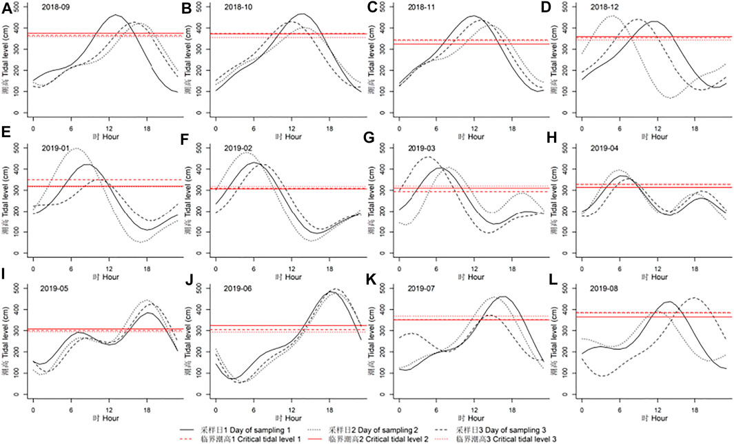
FIGURE 2. (A)The distribution of tidal levels and critical tidal levels in mangrove vegetation areas from September 2018 to August 2019.

3.1 Applicable algorithms for mangrove vegetation segmentation

Visual interpretation found that different segmentation algorithms had significant differences in sensitivity to mangroves and background information. The algorithms based on color space, nonlinear combination of color channels, and machine learning could highly distinguish the bright green mangroves in the close-range view, and the differences in segmentation results were not significant. However, differences became significant when using the algorithms to distinguish the mud flat in close-range view and grrayish-green mangroves in distant-range view, which were in the order of machine learning > channel S > channela > ExG (Figure 3).

FIGURE 3

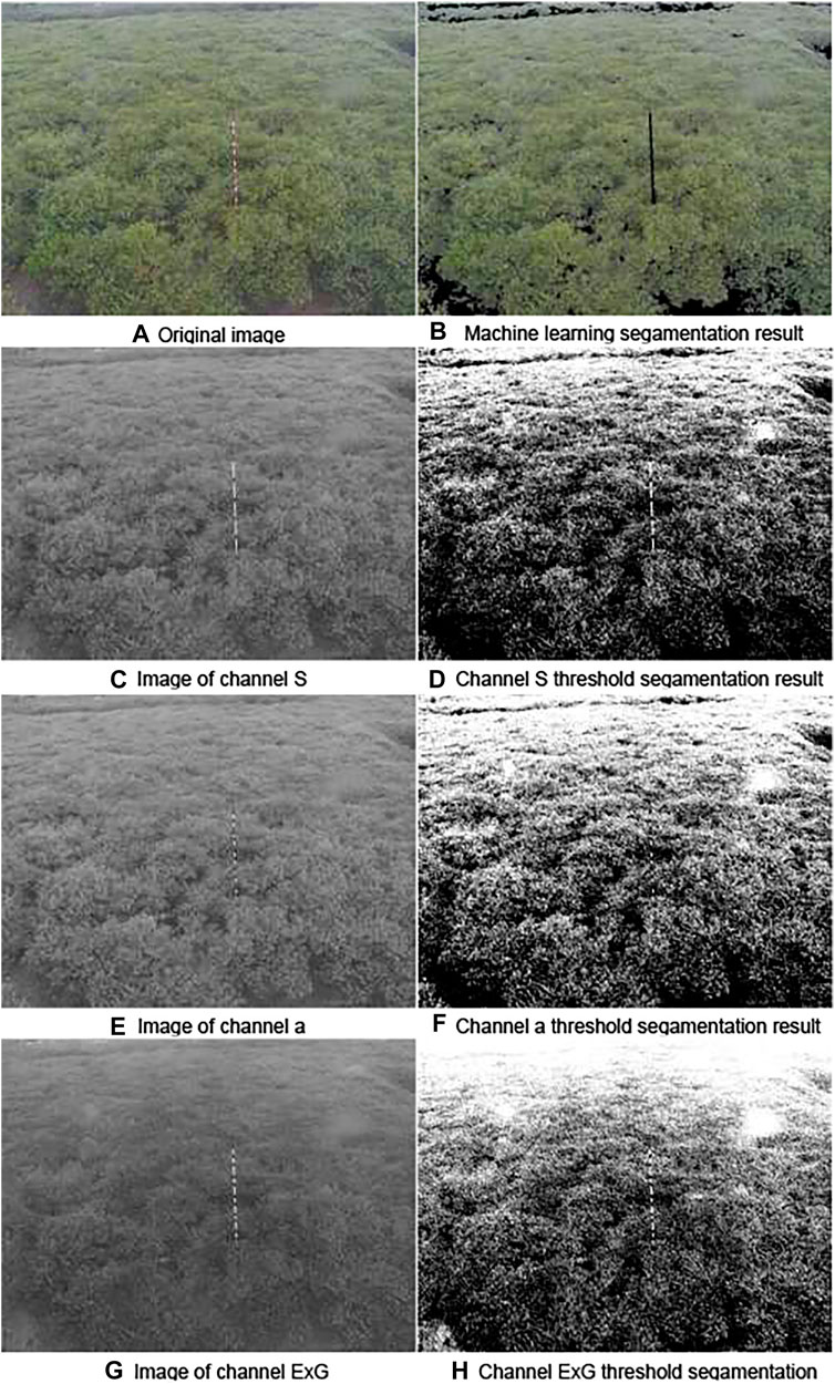
FIGURE 3. Segmentation effects of mangrove vegetation images. (A) Original image. (B) Machine learning segmentation result. (C) Image of channel S. (D) Channel S threshold segmentation result. (E) Image of channel a. (F) Channel a threshold segmentation result. (G) Image of channel ExG. (H) Channel ExG threshold segmentation.

The accuracy of machine learning algorithm for segmentation of mangrove vegetation was better than other algorithms. Machine learning also showed the best segmentation effect when using field labeling results as a reference to quantitatively analyze the segmentation accuracy of the three kinds of algorithms, with the Qseg and Sr of 80.56% and 86.46%, respectively, and the accuracy rates of other segmentation algorithms were lower than 80%, of which EXG showed the poorest segmentation effect with the Qseg and Sr of 73.60% and 75.45%, respectively (Table 1).

NLM filtering could effectively optimize various segmentation results. After filtering processing, the error segmentation of background information, such as mangrove leaf edges and mudflats, were significantly reduced, with an Qseg increase of 0.88%–1.15% and Sr increase of 0.81%–1.61%. The optimization effect was the most significant on the segmentation results of channel S, and the accuracy was improved the most after filtering. Considering the overall performances, machine learning was used for the original RGB image segmentation and NLM filtering optimization strategy. In this way, the final segmentation accuracy of mangrove vegetation could reach 87.27% (Table 2).

TABLE 2

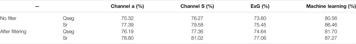
TABLE 2. Comparison on accuracy of mangrove vegetation image segmentation algorithms.

3.3 Applicable monitoring index for mangrove growth monitoring

The 10 RGB vegetation indices could be divided into two categories according to their sequential variation characteristics. The first category contained the indices with seasonal changes that were quasisynchronous with temperature changes (collectively referred to as seasonal indices), including ExG, ExGR, GLA, GMRVI, NDYI, RGBVI, VARI, and VEG. The indices in this category have lower values in winter and spring, while they have higher values in summer and autumn. The second category was the indices with seasonal change trend that was opposite to the temperature change over time (collectively referred to as the antiseasonal indices), including ExR and CIVE. The indices in this category had lower values in summer and autumn, but higher values in winter and spring, which was opposite to the seasonal indices (Figure 4).

FIGURE 4

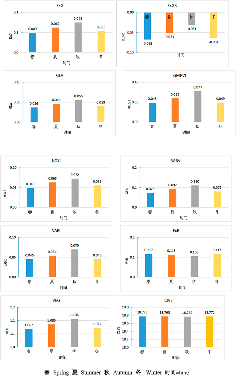
FIGURE 4. Seasonal changes of mangrove visible vegetation index.

Compound sine function could better simulate the periodic changes in various RGB vegetation indices during the year. The correlation coefficients between the simulated and observed values of various indices were between 0.430 and 0.643, among which VARI had the best fitting effect (R = 0.643), and ExG had the worst fitting effect (R = 0.505). The annual sequence fitting deviations of various indices were between 0.03% and 26.16%, among which ExR (4.09%), VEG (1.73%), and CIVE (0.03%) showed relatively small deviations between the fitted values and observed values, while the deviations of other indices were all greater than 17% (Figure 5; Table 3).

FIGURE 5

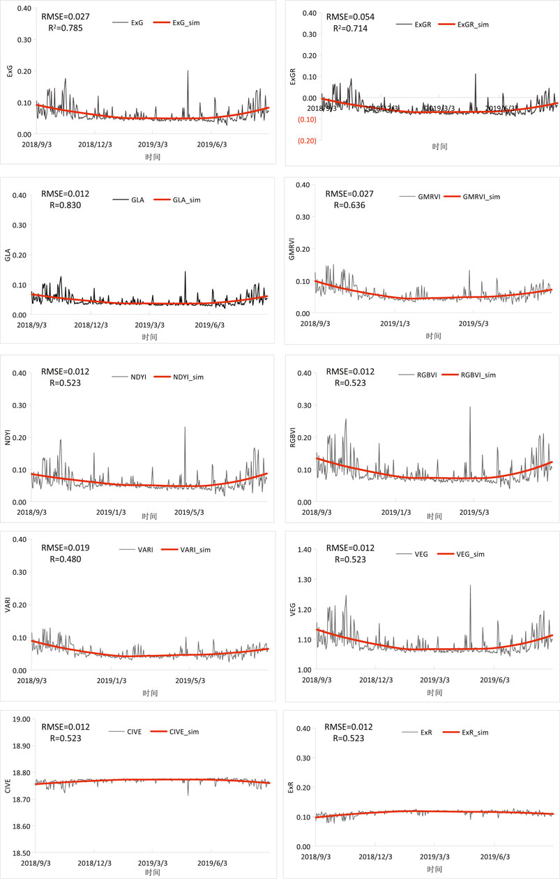
FIGURE 5. Time variations of mangrove RGB vegetation index.

TABLE 3

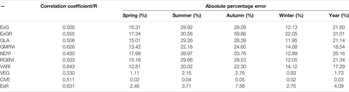
TABLE 3. Correlation and deviation percentage between fitted and observed values of mangrove RGB vegetation indices.

The simulated results of various RGB vegetation indices fitted by the compound sine function showed significant differences in seasons. The deviation was 0.02%–17.98% in spring, 0.04%–39.97% in summer, 0.05%–59.66% in autumn, and 0.02%–22.05% in winter. In comparison, the deviations were small in winter and spring, and large in summer and autumn (Table 3). Therefore, seasonal index VEG and antiseasonal index CIVE could be used as the preferred indices for mangrove growth monitoring. The reasons were that, as one of the seasonal indices, VEG made it easier to understand the impact of weather conditions on mangrove growth, while CIVE, an antiseason index, had smaller simulation deviation.

3.4 Response of mangrove growth monitoring indices to meteorological factors

The selected main meteorological factors were daily average temperature, daily maximum temperature, daily minimum temperature, relative humidity, and daily precipitation, which were used to make correlation analysis with mangrove canopy RGB vegetation indices (Table 4). There was a high degree of correlation among various RGB vegetation indices (Table 5), but due to the difference in image bands and parameters, the correlations between different RGB vegetation indices and meteorological factors were significantly different. The eight seasonal RGB vegetation indices (ExG, ExGR, GLA, GMRVI, NDYI, RGBVI, VARI, and VEG) were positively correlated with average temperature, maximum temperature, minimum temperature, and precipitation, and negatively correlated with relative humidity, while the correlations between the two counterseasonal RGB vegetation indices (ExR and CIVE) and the meteorological factors were opposite to those of the seasonal indices. Among them, ExR, VARI, MGRVI, and NGRDI showed significant correlations with temperature (average, maximum, and minimum) and relative humidity, while NDYI and CIVE showed no significant correlation with temperature and relative humidity. In terms of precipitation, the correlation with NDYI, GLA, RGBVI, CIVE, and VEG reached significant levels, while the other RGB vegetation indices were not significantly correlated. In general, the RGB vegetation indices were sensitive to meteorological factors, and thus, they could be used to analyze the influence of meteorological conditions on the growth of mangroves.

TABLE 4

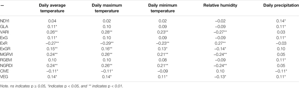
TABLE 4. Correlation between mangrove RGB vegetation indices and meteorological factors.

TABLE 5

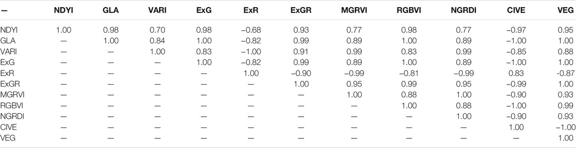
TABLE 5. Correlation comparison of mangrove RGB vegetation indices.

4 Discussion

Machine learning algorithm can improve the segmentation accuracy of mangrove vegetation in aerial RGB images, and this result has been confirmed in the research on the segmentation of UAV images of mangroves at the park scale (Wen et al., 2020). Digital cameras can be used to monitor the critical tidal levels of mangrove submersion, and the exposure time of mangroves in the test area is significantly longer than the submerging time (Figure 4), which further proved the results of a previous research on the seawater submerging rules of mangroves (Zhang and Zheng, 1997; Chen et al., 2006). Under the combined effects of light, precipitation, and seawater submersion, the daily RGB vegetation indices of mangrove vegetation vary greatly, but there is still a significant seasonal trend. However, since the peak time is mostly in autumn, there is a certain difference in the time with peak value of temperature. The day-to-day vegetation indices extracted using visible images vary greatly. The possible reasons are as follows: Mangroves are located in the intertidal zone, and both seawater submersion and extreme weather will have severe impacts on the vegetation indices of the coastal zone (Wang, 2017), and the digital camera equipped in the ecological station performs automatic exposure and correction according to the light conditions when collecting images, and different exposure times can cause large differences in the quality of vegetation images (Wang et al., 2016).

In this study, we combine image processing with machine learning technology to provide effective technical methods for automatic and continuous monitoring of mangrove vegetation conditions, but there are still many shortcomings. First, limited by the test conditions, the onsite labeling results are used as the references for the evaluation on the accuracy of various segmentation algorithms, but there is no onsite surveys and sample sampling of the study area. Second, using visual interpretation to determine the submerging status of mangroves can result in low image data processing efficiency. In further research, multispectral cameras equipped to the ground-based and UAV platforms can be used to obtain multispectral and hyperspectral data, and sampling plots can be set in the study area to collect the data related with the physical and chemical properties of plants, so as to enrich the ground data set. Setting camera parameters and improving image correction methods can reduce the variability of RGB vegetation indices. The construction of a prediction model based on the biomass, leaf area index, and chlorophyll content of RGB vegetation indices can provide technical support for real-time, fast, and accurate estimation of mangrove vegetation growth parameters.

5 Conclusion

The visible images obtained by the ground camera can be used to carry out quantitative monitoring of mangrove growth, which can be achieved by three processes: image screening, vegetation segmentation, and RGB vegetation index calculation.

Image screening can be carried out by using two key indicators: critical tide level and image brightness. The start time of the mangrove submersion in the study area shows a cyclical change with the passage of time, which is delayed first and shifted to an earlier time. On such basis, the average critical tidal level is 334.8 cm in the observation point. The image brightness value is represented by the sum of values of R, G, and B color channels.

Machine learning and NLM filtering are effective strategies to obtain high-precision mangrove segmentation results. The machine learning segmentation algorithm has superiority in the automatic segmentation of mangrove vegetation, and the accuracy of the segmentation results is higher than 80% without filtering. NLM filtering can effectively optimize the segmentation results of various algorithms.

Mangrove RGB vegetation indices include seasonal indices and counterseasonal indices synchronized with temperature changes. Seasonal index VEG and counterseasonal index CIVE can be used as preferred indexes for mangrove growth monitoring. The compound sine function can better simulate the change trend of various RGB vegetation indices, and the simulation effect in winter and spring is better than that in summer and autumn.

The RGB vegetation indices can be used to analyze the effect of meteorological conditions on the growth of mangroves. The RGB vegetation indices of mangroves are sensitive to meteorological factors. Among them, seasonal RGB vegetation indices show positive correlations with average temperature, maximum temperature, minimum temperature, and precipitation, but show negative correlation with relative humidity. On the other hand, the correlations between counterseasonal RGB vegetation indices and the various meteorological factors are opposite to those of the seasonal indices.

Data Availability Statement

The raw data supporting the conclusions of this article will be made available by the authors, without undue reservation.

Author Contributions

YC wrote the thesis. SF reviewed the manuscript and designed the framework. MS, ZL, LP, WM and CC assisted in the data processing.

Funding

The study is supported by the Open Research Fund Program of Guangxi Key Lab of Mangrove Conservation and Utilization (GKLMC-202004), the Special Project for Climate Change of China Meteorological Administration (CCSF202030), and the Key Project of Fundamental Research Funds (2019Z010).

Conflict of Interest

The authors declare that the research was conducted in the absence of any commercial or financial relationships that could be construed as a potential conflict of interest.

Publisher’s Note

All claims expressed in this article are solely those of the authors and do not necessarily represent those of their affiliated organizations, or those of the publisher, the editors, and the reviewers. Any product that may be evaluated in this article, or claim that may be made by its manufacturer, is not guaranteed or endorsed by the publisher.

References

Bendig, J., Yu, K., Aasen, H., Bolten, A., Bennertz, S., Broscheit, J., et al. (2015). Combining UAV-Based Plant Height from Crop Surface Models, Visible, and Near Infrared Vegetation Indices for Biomass Monitoring in Barley. Int. J. Appl. Earth Observation Geoinformation 39, 79–87. doi:10.1016/j.jag.2015.02.012

CrossRef Full Text | Google Scholar

Campillo, C., Prieto, M. H., Daza, C., Moñino, M. J., and García, M. I. (2008). Using Digital Images to Characterize Canopy Coverage and Light Interception in a Processing Tomato Crop. horts 43, 1780–1786. doi:10.21273/hortsci.43.6.1780

CrossRef Full Text | Google Scholar

Cao, Q. X. (2017). Remote Sensing Estimation of Mangrove Biomass and Carbon Storage in the Beibu Gulf Coast[J]. Chin. Acad. For. 24 (2), 144–149. doi:10.13656/j.cnki.gxkx.20170411.002

CrossRef Full Text | Google Scholar

Chen, L., Ding, G. H., and Guo, L. (2011). Image Thresholding Based on Mutual Confirmation of Histogram[J]. J. Infrared Millimeter Waves 30 (1), 80–84. doi:10.3724/sp.j.1010.2011.00080

CrossRef Full Text | Google Scholar

Chen, L., Yang, Z., Wang, W., and Lin, P. (2006). Critical Tidal Level for Planting Kandelia candel Seedlings in Xiamen. Ying Yong Sheng Tai Xue Bao 17 (2), 177–181. doi:10.13287/j.1001-9332.2006.0036

PubMed Abstract | CrossRef Full Text | Google Scholar

Chen, M., Zheng, S. F., Liu, X. L., Xu, D. Q., Wang, W., and Kan, H. C. (2017). Cotton Nitrogen Nutrition Diagnosis Based on Digital Image[J]. J. Agric. 7 (7), 77–83.

Google Scholar

Gitelson, A. A., Kaufman, Y. J., Stark, R., and Rundquist, D. (2002). Novel Algorithms for Remote Estimation of Vegetation Fraction. Remote Sensing Environ. 80 (1), 76–87. doi:10.1016/s0034-4257(01)00289-9

CrossRef Full Text | Google Scholar

Guijarro, M., Pajares, G., Riomoros, I., Herrera, P. J., Burgos-Artizzu, X. P., and Ribeiro, A. (2011). Automatic Segmentation of Relevant Textures in Agricultural Images. Comput. Electron. Agric. 75 (1), 75–83. doi:10.1016/j.compag.2010.09.013

CrossRef Full Text | Google Scholar

Hague, T., Tillett, N. D., and Wheeler, H. (2006). Automated Crop and Weed Monitoring in Widely Spaced Cereals. Precision Agric. 7 (1), 21–32. doi:10.1007/s11119-005-6787-1

CrossRef Full Text | Google Scholar

Han, D., Wu, H. J., Ma, Z. Y., Han, G. D., Wu, P., and Zhang, Q. (2019). Feature Extraction and Recognition of Typical Pastures in Grassland[J]. Chin. J. Grassland 41 (4), 128–135. doi:10.16742/j.zgcdxb.20190043

CrossRef Full Text | Google Scholar

Jones, A. R., Segaran, R. R., Clarke, K. D., Waycott, M., Goh, S. H., Gillanders, B. M., et al. (2020). Estimating Mangrove Tree Biomass and Carbon Content: a Comparison of forest Inventory Techniques and Drone Imagery[J]. Front. Mar. Sci. 6, 13. doi:10.3389/fmars.2019.00784

CrossRef Full Text | Google Scholar

Kataoka, T., Kaneko, T., Okamoto, H., and Hata, S. (2003). “Crop Growth Estimation System Using Machine Vision[J],” in IEEE/ASME International Conference on Advanced Intelligent Mechatronics, Kobe, Japan, 20-24 July 2003 (IEEE), b1079–b1083.

Google Scholar

Kovacs, J. M., Wang, J., and Flores-Verdugo, F. (2005). Mapping Mangrove Leaf Area index at the Species Level Using IKONOS and LAI-2000 Sensors for the Agua Brava Lagoon, Mexican Pacific. Estuarine, Coastal Shelf Sci. 62, 377–384. doi:10.1016/j.ecss.2004.09.027

CrossRef Full Text | Google Scholar

Li, J., Jiang, N., Baoyin, B. T., Zhang, F., Zhang, W. J., and Wang, W. (2020). Spatial Color Clustering Algorithm and its Application in Image Feature Extraction[J]. J. Jilin Univ. (Science Edition) 58 (3), 627–633. doi:10.13413/j.cnki.jdxblxb.2019282

CrossRef Full Text | Google Scholar

Liu, S. Y., Li, L., Te, R. G., Li, Z. Q., Ma, J. Y., and Zhu, R. F. (2021). Threshold Segmentation Algorithm Based on Histogram Area Growing for Remote Sensing Images[J]. Bull. Surv. Mapp. (2), 25–29. doi:10.13474/j.cnki.11-2246.2021.0037

CrossRef Full Text | Google Scholar

Liu, Z. P., Kuang, S. W., Ma, R. S., Wu, X. K., Wang, D., Li, L., et al. (2020). Study on Automatic Recognition Technology of Sugarcane Emergence Stage Based on Image Features[J]. Sugarcane and Canesugar 49 (5), 41–46.

Google Scholar

Lu, M., Shen, S. H., Wang, C. Y., and Li, M. S. (2011). Initial Exploration of maize Phenological Stage Based on Image Recognition[J]. Chin. J. Agrometeorology 32 (3), 423–429. doi:10.3969/j.issn.1000-6362.2011.03.017

CrossRef Full Text | Google Scholar

Ma, B. Y., Liu, C. N., Gao, M. F., Ban, X. J., Huang, H. Y., Wang, H., et al. (2020). Region Aware Image Segmentation for Polycrystalline Micrographic Image Using Deep Learning[J]. Chin. J. Stereology Image Anal. 25 (2), 120–127. doi:10.13505/j.1007-1482.2020.25.02.004

CrossRef Full Text | Google Scholar

Ma, X., Qi, L., and Zhang, X. C. (2008). Segmentation Technology of Exserochilum Turcicum Image Based on Fuzzy Clustering Analysis[J]. J. Agric. Mechanization Res. (12), 24–26. doi:10.3969/j.issn.1003-188X.2008.12.007

CrossRef Full Text | Google Scholar

Meyer, G. E., Hindman, T. W., and Laksmi, K. (1999). Machine Vision Detection Parameters for Plant Species Identification[J]. Precision Agric. Biol. Qual., 327–335. doi:10.1117/12.336896

CrossRef Full Text | Google Scholar

Min, L., Gao, K., Li, W., Wang, H., Li, T., Wu, Q., et al. (2020). A Review of Optical Remote Sensing Image Segmentation Technology[J]. Spacecraft Recovery & Remote Sensing 41 (6), 1–13. doi:10.3969/j.issn.1009-8518.2020.06.001

CrossRef Full Text | Google Scholar

Ostu, N. (1979). A Threshold Selection Method from gray-level Histograms[J]. IEEE Trans. Syst. Man Cybernetcis 9 (1), 62–66. doi:10.1109/tsmc.1979.4310076

CrossRef Full Text | Google Scholar

Pérez, A. J., López, F., Benlloch, J. V., and Christensen, S. (2000). Colour and Shape Analysis Techniques for weed Detection in Cereal fields. Comput. Electron. Agric. 25 (3), 197–212. doi:10.1016/s0168-1699(99)00068-x

CrossRef Full Text | Google Scholar

Peter, J., Hogland, J., Hebblewhite, M., Hurley, M., Hupp, N., and Proffitt, K. (2018). Linking Phenological Indices from Digital Cameras in Idaho and Montana to MODIS NDVI. Remote Sensing 10, 1612. doi:10.3390/rs10101612

CrossRef Full Text | Google Scholar

Purcell, L. C. (2000). Soybean Canopy Coverage and Light Interception Measurements Using Digital Imagery. Crop Sci. 40, 834–837. doi:10.2135/cropsci2000.403834x

CrossRef Full Text | Google Scholar

Ramsey, E. W., and Jensen, J. R. (1996). Remote Sensing of Mangrove Wetlands: Relating Canopy Spectra to Site-specific Data[J]. Photogrammetric Eng. Remote Sensing 62 (31), 939–948.

Google Scholar

Ren, J., Li, Z. N., and Fu, Y. P. (2004). Edge Detection of Color Images Based on Wavelet and Reduced Dimensionality Model of RGB[J]. J. Zhejiang Univ. (Engineering Science) 38 (7), 856–859+892. doi:10.3785/j.issn.1008-973X.2004.07.014

CrossRef Full Text | Google Scholar

Shi, P. H., Wang, Y., Yuan, Z. Q., Sun, Q. Y., Cai, S. Y., and Lu, X. Z. (2020). Winter Wheat Nitrogen Nutrition index Based on Canopy RGB Image[J]. J. Nanjing Agric. Univ. 43 (5), 829–837. doi:10.7685/jnau.202001020

CrossRef Full Text | Google Scholar

Sulik, J. J., and Long, D. S. (2016). Spectral Considerations for Modeling Yield of Canola. Remote Sensing Environ. 184, 161–174. doi:10.1016/j.rse.2016.06.016

CrossRef Full Text | Google Scholar

Wang, C. Y., Guo, X. Y., Wen, W. L., Du, J. J., and Xiao, B. X. (2016). Application of Hemispherical Photography on Analysis of maize Canopy Structural Parameters under Natural Light[J]. Trans. Chin. Soc. Agric. Eng. 32 (4), 157–162. doi:10.11975/j.issn.1002-6819.2016.04.022

CrossRef Full Text | Google Scholar

Wang, X. L. (2017). Spatiotemporal Variations of Extreme Climate Events and Their Impacts on NDVI in Coastal Area of China[D]. University of Chinese Academy of Sciences. Doctoral dissertation

Google Scholar

Wen, X., Jia, M. M., Li, X. Y., Wang, Z. M., Zhong, C. R., and Feng, E. H. (2020). Recognition of Mangrove Canopy Species Based on Visible Unmanned Aerial Vehicle Images[J]. J. For. Environ. 40 (5), 486–496. doi:10.13324/j.cnki.jfcf.2020.05.005

CrossRef Full Text | Google Scholar

Woebbecke, D. M., G. E. Meyer, G. E., K. Von Bargen, K. V., and Mortensen, D. A. (1995). Color Indices for Weed Identification under Various Soil, Residue, and Lighting Conditions. Trans. Asae 38 (1), 259–269. doi:10.13031/2013.27838

CrossRef Full Text | Google Scholar

Wu, L. F., Wang, M. G., Fu, H., and Jian, M. (2018). Automatic Recognition of Cotton Growth by Combining Deep Learning Based Object Recognition and Image Classification[J]. Chin. Sci. Technol. Paper 13 (20), 2309–2316. doi:10.3969/j.issn.2095-2783.2018.20.005

CrossRef Full Text | Google Scholar

Wu, Q. (2014). Research on Automatic Detection of Cotton Growth Stages by Image Processing technology[D]. Hubei: Huazhong University of Science and Technology.

Google Scholar

Yan, C., Sun, Z. Q., Tin, E. G., Zhao, Y. Y., and Fan, X. Y. (2021). Research Progress of Medical Image Segmentation Based on Deep Learning [J]. Electron. Sci. Technol. 34 (2), 7–11. doi:10.16180/j.cnki.issn1007-7820.2021.02.002

CrossRef Full Text | Google Scholar

Yang, H., Zhao, J., Lan, Y., Lu, L., and Li, Z. (2018). Fraction Vegetation Cover Extraction of winter Wheat Based on RGB Image Obtained by UAV. Int. J. Precision Agric. Aviation 1 (1), 54–61. doi:10.33440/j.ijpaa.20190202.44

CrossRef Full Text | Google Scholar

Zhang, Q. M., and Zheng, D. Z. (1997). The Relationship between Mangrove Zone and Tidal Flats and Tidal Levels[J]. Acta Ecologica Sinica 17 (3), 258–265.

Google Scholar

Zhang, W. (2016). Monitoring the Areal Variation of Mangrove in Beibu Guff Coast of Guangxi China with Remote Sensing Data[J]. J. Guangxi Univ. (Natural Sci. Edition) 40 (6), 1570–1576. doi:10.13624/j.cnki.issn.1001-7445.2015.1570

CrossRef Full Text | Google Scholar

Zhou, H. J., Liu, Y. D., Fu, J. D., Sui, F. G., and Zhu, R. X. (2015). Analysis of maize Growth and Nitrogen Nutrition Status Based on Digital Camera Images[J]. J. Qingdao Agric. Univ. (Natural Sci. Edition) 32 (1), 1–7. doi:10.3969/J.ISSN.1674-148X.2015.01.001

CrossRef Full Text | Google Scholar

Zhu, Y. H., Liu, L., Liu, K., Wang, S. G., and Ai, B. (2014). Progress in Researches on Plant Biomass of Mangrove Forests[J]. Wetland Sci. 12 (4), 515–526. doi:10.13248/j.cnki.wetlandsci.2014.04.016

CrossRef Full Text | Google Scholar

Zhu, Y., Liu, K., Myint, S. W., Du, Z., Li, Y., Cao, J., et al. (2020). Integration of GF2 Optical, GF3 SAR, and UAV Data for Estimating Aboveground Biomass of China's Largest Artificially Planted Mangroves. Remote Sensing 12 (12), 2039. doi:10.3390/rs12122039

CrossRef Full Text | Google Scholar