A Song of Neither Ice nor Fire: Temperature Extremes had No Impact on Violent Conflict Among European Societies During the 2nd Millennium CE

The second millennium CE in Europe is known for both climatic extremes and bloody conflict. Europeans experienced the Medieval Warm Period and the Little Ice Age, and they suffered history-defining violence like the Wars of the Roses, Hundred Years War, and both World Wars. In this paper, we describe a quantitative study in which we sought to determine whether the climatic extremes affected conflict levels in Europe between 1,005 and 1980 CE. The study involved comparing a well-known annual historical conflict record to four published temperature reconstructions for Central and Western Europe. We developed a Bayesian regression model that allows for potential threshold effects in the climate–conflict relationship and then tested it with simulated data to confirm its efficacy. Next, we ran four analyses, each one involving the historical conflict record as the dependent variable and one of the four temperature reconstructions as the sole covariate. Our results indicated that none of the temperature reconstructions could be used to explain variation in conflict levels. It seems that shifts to extreme climate conditions may have been largely irrelevant to the conflict generating process in Europe during the second millennium CE.

Introduction

“Winter is coming”, the motto of House Stark in George R.R. Martin’s A Song of Ice and Fire series of epic fantasy novels, is an ominous metaphorical portent of difficult times to come. The novels were inspired by the historical events of the Wars of the Roses (DiPaolo, 2018), a series of conflicts in Late Medieval England that began in 1455 CE (Hicks, 2012). These conflicts erupted shortly after the onset of the Little Ice Age, a period during which average temperatures in the Northern Hemisphere dropped by around 0.5°C in a few decades and then remained low for centuries (Mann et al., 2009). In light of these connections to historical events, the Stark’s motto can be read as an allegorical reference to the twin threats of anthropogenic climate change and the violent conflicts it may ignite (DiPaolo, 2018).

The idea that anthropogenic climate change will lead to more conflict has received increasing attention in recent years. It has been endorsed by a number of major policy organisations including the Inter-Governmental Panel on Climate Change (IPCC) (Adger et al., 2014), the US Department of Defense (2010), and the European Commission (2013). There has also been intense scientific interest in climate-conflict dynamics. Dozens of case studies have been published reporting quantitative analyses of conflict records and climatic variables. The conflict records include events ranging in scale and intensity from cattle raids to political uprisings and civil wars that occurred during various sub-intervals of the 20th and early 21st centuries CE. Surprisingly, though, results have been mixed (Koubi, 2019; Mach et al., 2019). Some studies have found that increases or decreases in temperature corresponded to increased conflict levels (i.e., incidence) (e.g., Zhang et al., 2006; Burke et al., 2009), while others reported mixed findings (e.g., Tol and Wagner, 2010) or no effect at all (e.g., Carleton et al., 2021). Similarly inconsistent findings have been reported with respect to the potential impact of rainfall variation on conflict levels (e.g., Theisen, 2012; Von Uexkull et al., 2016).

These contradictory findings are counter-intuitive. Environmental variables are clearly linked to economics, primarily through the impact of environmental variation on agricultural productivity and trade (Gornall et al., 2010). It seems that this should, in turn, affect the prevalence of violent conflicts between groups competing for access to increasingly scarce resources (e.g., Allen et al., 2016). If droughts, for instance, diminish agricultural productivity, then the resulting shortfall in the food supply and commodities might be expected to increase the odds that the negatively affected groups would attempt to compensate at times by taking the desired resources from others (e.g., Burke et al., 2009). Reluctance to hand over resources would then give rise to organised violent conflicts. Scholars of international relations and conflict and peace researchers have referred to this putative causal chain as a “scarcity mechanism’ and it has intuitive appeal (e.g., Glowacki and Wrangham, 2013; Koubi, 2019; Schmidt et al., 2021). Even in cases where compensatory strategies were available (e.g., alternate foods, trade), these would not always work as hoped—trade agreements fail and alternate resources are not always sufficient. In addition, the scarcity mechanism would still produce higher levels of conflict given enough time or a large enough focal region. This is because the odds of conflict occurring would still be elevated, which ultimately means more conflicts on average. That recent research has so far failed to find evidence for a universal relationship between temperature and conflict levels is, therefore, surprising.

This situation has led some researchers to highlight the importance of longer-term records (e.g., Buhaug, 2015; Koubi, 2019). The suggestion makes sense because there are differences between records with different time horizons. Short-term records of conflict incidence, for instance, are likely to be highly erratic with respect to causation. Individual conflicts can happen for numerous reasons that vary among incidents. Additionally, there is a well-known pattern of autocorrelation in conflict data (Richardson, 1944; Houweling and Siccama, 1985; Brandt et al., 2000). Such autocorrelation means that a high level of conflict in one period can predict the level of conflict in subsequent periods. This pattern may occur simply because conflicts beget further conflicts as opponents retaliate for past aggression, which makes it difficult to attribute changes in conflict levels to external factors. Similar features are present in climatological data (Vasseur and Yodzis, 2004). Day-to-day variation in climatological observations cannot necessarily be attributed to changes in long-term patterns. At the same time, the temperature or precipitation in one interval is usually correlated with the temperature or precipitation in previous intervals—i.e., there tends to be autocorrelation in climatolological processes, too. These common features of conflict and climate processes create challenges for seeing meaningful persistent signals in short runs of observations because the records can be noisy and explained by previous observations alone. Consequently, it can be difficult to detect persistent and significant covariation between conflict records and climate change if only short intervals are considered.

Unfortunately, however, the inconsistency persists even when considering long-term conflict and climate records. To our knowledge, there are three major long-term historical case studies available for comparison. Each includes a conflict record spanning multiple centuries that has been analysed quantitatively. One is the epigraphic (monument inscriptions) record of Classic Maya conflict spanning more than 600 years (ca 250–900 CE) (Kennett et al., 2012); another involves more than 2000 years of Chinese conflict records (ca. 800 BCE–1911 CE) (Zhang et al., 2006); and the third involves nearly 1,000 years of conflict among central and western European societies (ca. 1,000–1980 CE) (Tol and Wagner, 2010). Recent studies involving the Classic Maya epigraphic data have found that increased temperatures corresponded to increased conflict while annual precipitation had no apparent effect (Carleton et al., 2017; Collard et al., 2021). Analyses of the Chinese historical data, on the other hand, found that decreasing temperature corresponded to increased conflict levels (Zhang et al., 2006). Lastly, studies involving the conflict data for second millennium CE Europe have found either weak evidence for an effect of climate change on conflict (Tol and Wagner, 2010) or no evidence at all (Carleton et al., 2021).

The last of these cases is particularly interesting. Europe was repeatedly afflicted by wars during the second millennium CE (Tallett and Trim, 2010). These include the Hundred Years War—a series of wars between Medieval England and France from 1,337 to 1453 CE (Green, 2014)—and the aforementioned Wars of the Roses from 1,455 to 1487 CE (Hicks, 2012). These Late Medieval clashes were then followed by the European Wars of Religion between the 1520s and 1640s CE, multiple wars with the Ottoman Empire, numerous revolutionary wars, the Napoleonic Wars, and of course the two world wars of the 20th century CE (Neiberg, 2003; Black, 2007; Tallett and Trim, 2010). The period was also punctuated by bouts of climate change. The beginning of the millennium witnessed a relatively warm period in much of Europe. Known today as the Medieval Warm Period (or Medieval Climate Anomaly), this lasted from about 950 to 1250 CE (Crowley and Lowery, 2000; Mann et al., 2009). Subsequently, around 1400 CE, the continent was plunged into the Little Ice Age, a deep cold that lingered into the early 19th century CE (Mann et al., 2009) with some parts of the Northern Hemisphere experiencing as much as a 4°C drop in average temperatures in a few decades (D’Andrea et al., 2011). The conflicts that occurred during these substantial swings in climatic conditions were in part fought over access to wealth and they required resources to initiate and sustain. It is, therefore, striking that the aforementioned studies found the association between climate change and conflict levels to be weak to non-existent.

There are several possible explanations for the failure of previous research to find a relationship between climate conditions and historical European conflict levels. One might involve biases in the conflict and/or climate records, for example. Another explanation might be that analyzing aggregated data for the whole of Western Europe obscured important local or regional differences in one or more variables, leading to a falsely negative signal about the climate-conflict relationship. A third explanation may be that the scarcity hypothesis is simply wrong, or points to an effect that is eclipsed by other factors like greed, prestige, and politics. Lastly, it could be that the statistical models used so far are too simplistic to identify the relationship between climate and conflict. As Carleton et al. (2021) point out, some of these explanations can be discounted by careful reasoning while others are harder to evaluate at present and should be the subject of future research.

In the present paper, we describe a study in which we explored an important avenue for future research identified by Carleton et al. (2021): the potentially unique impact of extreme climate conditions on conflict levels. Both Tol and Wagner (2010) and Carleton et al. (2021) employed regression models that assume the relationship between climate variation and conflict levels was constant for all levels of the climate variable, temperature being the key proxy for climate change in both cases. This assumption may have led to the analyses missing a threshold effect. It is possible that for moderate temperatures the European conflict process was dominated by non-climatic factors. These might have included retaliation or purely political motivations among those involved. But, during periods of extreme temperatures—say, the coldest intervals of the Little Ice Age—climate variation could plausibly have become much more important.

To explore this possibility, we revised the time-series model used in Carleton et al. (2021) so that it could identify threshold effects. As with the previous model, the new one is Bayesian and employs an autocorrelation term to reflect the “memory” present in the conflict record and allows for covariates to potentially explain any remaining variation in the record not better accounted for by autocorrelation. The new model, however, also employs a “broken-stick” regression framework for the covariates—the “broken stick” refers to connected regression lines that can have different slope values. The model creates the separate “sticks” by fitting two thresholds to the independent variable, one upper and one lower. These thresholds allow for three different ranges of covariate values. A separate regression coefficient (i.e., slope) can then be estimated for each of the three ranges (the three sticks). The separate regression functions make it possible for a given independent variable to have a different relationship to conflict over each of the ranges defined by the thresholds. Therefore, the relationship between conflict levels and a given covariate can be non-linear over the whole covariate range. Conflict levels, for example, could have a U-shaped relationship with temperature in the model, which would mean that conflicts were only significantly higher when temperatures were extreme and effectively random otherwise. Importantly, the model’s parameters (including threshold locations and slopes) are all estimated simultaneously from the data. Thus, the estimated values reflect the combined likelihood of those parameter values given all of the data. After adjusting the model, we used it to compare a well-known time-series of European conflict levels (incidents per year) during the second millennium CE to four temperature time-series.

Materials and Methods

The Data

The conflict record utilised in the present study was first analysed by Tol and Wagner (2010) in their influential investigation of climate-conflict dynamics. The record was recently reanalysed in the aforementioned paper by Carleton et al. (2021). The copy of the record we analysed was kindly provided by Richard Tol.

Tol and Wagner (2010) record contains an annual count of wars and battles between 1,000 and 2000 CE, with a conflict being counted in each year it was ongoing (Figure 1). Tol and Wagner (2010) compiled the record from entries in three databases: 1) Peter Brecke’s catalogue of historical conflicts (https://brecke.inta.gatech.edu/research/conflict/); 2) the Uppsala Conflict Data Program (https://ucdp.uu.se/); and 3) the COSIMO database (hosted by Heidelberg Institute for International Conflict Research—HIIK) (https://hiik.de/). In total, the Tol and Wagner (2010) record includes 3,450 conflict-year events from 1,000 to 1999 CE—there are fewer uniquely named historical conflicts than conflict-years because a conflict is counted in every year in which it occurred. Like Tol and Wagner (2010) and Carleton et al. (2021), we limited the record to the period from 1,005 to 1980 in order to ensure complete temporal overlap with the available temperature reconstructions. The restriction reduced the counts by a small amount, from 3,450 to 3,367 conflict-year events.

FIGURE 1

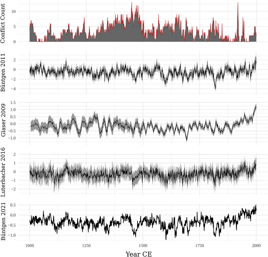
FIGURE 1. Time series data used in this study. Where available, we include confidence intervals for the climate data (middle three panels) and those are represented by lighter grey ribbons.

It is worth highlighting that this dataset represents only one dimension of violent conflict. The record comprises conflicts counted in a given year, as explained. In such a dataset, a border skirmish involving two states and a hundred soldiers would count as much as a larger war involving tens of thousands of combatants and multiple states. Our study, therefore, is only looking at conflict from one angle, namely conflict incidence. Other dimensions of conflict include onset, duration, number of warring parties, number of battle deaths, and so on. One reason for focusing on incidence as we did, though, was to ensure our results would be comparable with those of previous studies. Another reason is that the historical record contains more information about conflict dates than it does about the variables needed to assess the other dimensions of conflict. Filtering the dataset to only those historical conflicts where we know the number of battle deaths, for instance, would reduce the number of observations so much that meaningful patterns could no longer be extracted. After all, it can be difficult to estimate battle deaths from modern and recent wars let alone historical and ancient ones. Lastly, our intention was to evaluate whether climatic extremes led to an increase in per-period conflict levels as would be expected if the scarcity mechanism was a principle cause of variation. Importantly, according to that hypothesis, we would expect conflicts to start when resources became scarce and to persist (or be reignited) as long as they remained scarce, all else being equal. Such a relationship would be obscured by looking only at conflict onset. Consider a simple time-series of onset counts compared to a climate record. In that comparison, the climate variable could have an extreme value when the count was one (conflict begins) and the same extreme value when conflict count was zero (no new conflicts, despite continued fighting), which would imply no relationship between the two variables. For this reason and others, incidence is frequently used in conflict studies intended to identify relationships between overall conflict levels and external forces (Gleditsch et al., 2002; Hsiang et al., 2013). Consequently, in our view, the Tol and Wagner (2010) record was suitable for the study.

We compared the Tol and Wagner (2010) conflict record to four annual temperature reconstructions, the first three of which pertain specifically to Western and Central Europe and they were used in Carleton et al. (2021) as well (Figure 1). One of the temperature records was developed by Glaser and Reimann (2009) based on European historical documents. These documents include a variety of annals and personal diaries from different regions within Europe, though concentrated in the central and northern portions. The corpus includes descriptions of weather conditions as well as statements about crop yields. Glaser and Reimann (2009) categorised the descriptions into an ordinal temperature index, spanning approximately 1,000–1,800 CE, which they then calibrated using a instrumental data from 1761 to 1970 CE. Glaser and Reimann’s (Glaser and Riemann, 2009) index and the instrumental data are correlated with a Pearson’s R coefficient of 0.88.

The second temperature reconstruction was developed by Büntgen et al. (2011) and is based on high resolution tree-ring-width data. The widths were measured from 1,089 stone pine and 457 larch trees scattered throughout Europe, although like the previous historical data the spatial distribution is uneven with clusters in the central regions of relatively higher elevation. The reconstruction spans approximately 400 BCE to 2000 CE. The authors report Pearson’ R correlations in the range of 0.72–0.92 for the association between their reconstruction and instrumental data from 1864 to 2003.

The third temperature reconstruction was developed by Luterbacher et al. (2016) and is based on multiple lines of evidence. It is a product of the international PAGES 2k Consortium, a network of palaeoclimatologists who aim to create high-resolution climatic reconstructions (Turney et al., 2019). The source data include both tree-ring records and historical documents, some of which overlap with the data used for the previous two reconstructions. This composite reconstruction spans 138 BCE to 2003 CE. When the authors compared their reconstruction to instrumental data, they obtained Pearson R correlations on the order of 0.81–0.83. Luterbacher et al. (2016) produced two types of reconstruction and an average model. The average model is the one we used in the present study.

The fourth temperature time-series we included is a newly developed Northern Hemisphere tree-ring-based reconstruction (Büntgen et al., 2021). This time-series was constructed as part of a sizable community-based experiment in which the authors sought to determine how different methodological decisions affect tree-ring temperature reconstructions. The authors asked more than a dozen research groups to produce a reconstruction for the northern hemisphere and then compared the results. The reconstructions were based on tree-ring data from several sites around the Northern Hemisphere with a temporal ranges spanning the first two millennia CE. Ultimately, they determined that an ensemble mean most closely matched the instrumental record (with a Pearson R correlation of 0.79) and recommended using such ensemble means as a way of combating method-induced biases. In line with that recommendation, we decided to include the ensemble reconstruction in our analysis even though it likely registers hemispheric rather than European-specific temperature variation for the study period.

Defining Extremes

In order to explore the potential impact of “extreme” temperature values on conflict levels, we first needed to settle on a way of thinking about extremes in this context. Stewart et al. (this volume) conducted a large systematic survey of 200 journal articles in an effort to map out the ways in which extreme events in biological, societal, and Earth sciences have been studied. The review gave special attention to the quantitative and qualitative definitions used to operationalise extreme event research.

From their survey, Stewart et al. (this volume) determined that a common way of thinking about extremes involves deviations from reference (“normal”) conditions. In particular, research on temperature extremes—e.g., heat waves—commonly employs thresholds like the 95% confidence interval for temperatures compared to a given reference period. This 95% threshold is defined by a distribution of values where the bulk closest to the mean are considered “normal”. By way of contrast, extreme values deviate far from the mean, where “far” is defined by a threshold beyond which higher or lower values occur only 5% of the time or less in a random sample of measurements. Many studies also used a more effect-oriented way of thinking about extremes. Again, with respect to heatwaves for example, this effect-definition involved an established human biological heat tolerance threshold in degrees Celsius. The idea here is that, for biological reasons, temperatures in excess of this threshold lead to health problems and the relevant temperatures can, therefore, be considered “extreme”.

We decided that neither of these approaches would be appropriate for the present study. We were reluctant to employ a particular probability threshold (e.g., 95%) because the choice of such a threshold is arbitrary—why not use 90% or 99%? The second approach would not have worked either because we have no information about the temperature threshold(s) that might exist in the conflict generating process, at least not in Europe. Thus, we opted for a composite approach, one that combined the notion of deviations with data-driven estimation for the threshold values. Specifically, we scaled and centred all the of the temperature series, such that the values would represent deviations from the study-period-wide averages. Extremes among these scaled deviations were not defined a priori. Instead, we designed the time-series model to include the values of the potential thresholds as parameters to be estimated from the data.

The Broken-Stick Model

The time-series model, adapted from Carleton et al. (2021), is based on the Poisson distribution. It treats the count of conflicts, y, at a given time t as a conditionally independent observation from a latent conflict generating process. Thus,

$\begin{array}{ll}\hfill y_t& \sim Pois({\lambda }_t)\hfill \end{array}(1)$

$\begin{array}{ll}\hfill {\lambda }_t& =e^{r_t+{\mu }_t},\hfill \end{array}(2)$

where λ refers to the mean of the Poisson distribution.

The r_t term represents the autocorrelation in the conflict record. It is defined as a function of the previous level of the autocorrelation term, r_t−1, multiplied by a coefficient, ρ. Importantly, the model is stochastic and flexible enough to represent strictly autoregressive processes where ρ is between −1 and 1, and explosive or collapsing processes where ρ is greater than 1 or less than −1, respectively. This process can be expressed as follows,

$\begin{array}{ll}\hfill r_t& \sim N({\mu }_r,{\sigma }_r)\hfill \end{array}(3)$

$\begin{array}{ll}\hfill {\mu }_r& =r_{t-1}\rho \hfill \end{array}(4)$

$\begin{array}{ll}\hfill {\sigma }_r& \sim Exp(\cdot )\hfill \end{array}(5)$

$\begin{array}{ll}\hfill \rho & \sim N(\cdot )\hfill \end{array}(6)$

$\begin{array}{ll}\hfill r_0& \sim N(\cdot ).\hfill \end{array}(7)$

As this block of equations shows, there are several components to the autocorrelation process. The “(⋅)” notation is a placeholder for standard distribution parameters, while N () and Exp () refer to the Normal and Exponential distributions, respectively. The autocorrelation process has to have an initial level, denoted r₀, which is then fed into the equation for r₁. This term has a normal prior distribution with prior parameters for the mean and standard deviation, which we set to 0 and 2, respectively, and its most likely value is estimated from the data. Similarly, the autocorrelation coefficient, ρ, has a normal distribution with priors we set to 0 and 2 as well. The standard deviation of the autocorrelation process, σ_r, was given its own exponential prior distribution instead of using a fixed parameter value so that it could be estimated from the data. We opted for the exponential distribution because standard deviations must be positive by definition. This parameter controls the smoothness of the autocorrelation function. A large standard deviation would indicate a highly variable conflict generating process, which would make it very difficult to discern covariate impacts from intrinsic stochasticity. We assumed, therefore, that the background autocorrelation process is fairly smooth, which is reflected in our choice rate parameter (0.75) for the exponential prior.

The regression term in our model is represented by the μ_t parameter. Commonly in regression models, this parameter would be defined as follows,

$\begin{array}{ll}\hfill {\mu }_t& =x_t\beta \hfill \end{array}(8)$

$\begin{array}{ll}\hfill \beta & \sim N(\cdot ),\hfill \end{array}(9)$

where x_t is a covariate measurement at time t and β is a regression coefficient with a normal distribution—of course, x and β could be vectors referring to multiple covariates as well.

However, for the purposes of the present study, we needed to include thresholds for delineating extreme covariate values—the broken-stick regression (Feder, 1975, regarding broken stick models). Two thresholds were used to account for upper and lower extreme effects. These thresholds can be thought of as creating a set of conditions such that β could take on one value if x_t is above the upper threshold, τ⁺; another value if it is below the upper yet above the lower threshold, τ⁻; and, a third value if x_t is below the lower threshold. The thresholds define the points of articulation between the “broken sticks” (linear regression functions). We can represent this logic with different cases for μ_t:

${\mu }_t=\left\{\begin{array}{cc}{x}_t{\beta }^{+},\hfill & \text{if}{x}_t>{\tau }^{+}\hfill \\ x_t\beta ,\hfill & \text{if}{\tau }^{-}\le x_t\le {\tau }^{+}\hfill \\ x_t{\beta }^{-},\hfill & \text{if}{x}_t<{\tau }^{-},\hfill \end{array}\right.(10)$

given that τ⁺ > τ⁻. Assigning indicator functions, I (), to the cases makes for simpler computer code and can condense the above equations into a single one—these indicators are simply functions that equal 1 when a condition is met and zero otherwise, like a switch. Let I⁺(x_t) be a function that returns 1 when x_t > τ⁺ and zero otherwise. Along similar lines, let I⁻(x_t) return 1 when x_t < τ⁻ and zero otherwise. Then,

${\mu }_t=x_t(\beta +({\beta }^{+}{I}^{+}(x_t)+{\beta }^{-}{I}^{-}(x_t))),(11)$

which means that the model can fit different regression coefficients to different levels of the covariate using the mid-level coefficient, β, as a baseline. The other levels—β⁺ and β⁻—are then offsets from the baseline effect and have to be interpreted that way. These β parameters define the slopes of the articulating “sticks”.

The thresholds have to be given sensible priors and, in practice, need to be structured in such a way that they maintain their order so that the model remains identifiable. To that end, we defined the upper threshold first and then established the lower threshold by defining a differential parameter, d, that would be subtracted from the upper threshold. By then constraining d to be positive and non-zero we could ensure that the thresholds are properly estimated and always uniquely identifiable. Thus,

$\begin{array}{ll}\hfill {\tau }^{+}& \sim U(\cdot )\hfill \end{array}(12)$

$\begin{array}{ll}\hfill d& \sim U(\cdot )\hfill \end{array}(13)$

$\begin{array}{ll}\hfill {\tau }^{-}& ={\tau }^{+}-d.\hfill \end{array}(14)$

In these equations, U (⋅) refers to the uniform distribution with minimum and maximum bounds. Those boundaries are priors in the model. For τ⁺, we set the minimum boundary to 0 and the maximum to 5. We used these values because the covariates (i.e., temperature reconstructions) were mean-centred and scaled, as explained earlier. So, a value of 0 would refer to the study-period average against which extremes would be measured. We used a value of 5 for the maximum because none of the scaled temperature series exceeded |4| (akin to 4 standard deviations if the data were from a stationary normal distribution). The most extreme positive deviation, then, would have been upwards of 4, which meant that using 5 allowed for the possibility that the best fitting model included no upper threshold in the range of the observed data. The model, in effect, could push the boundary out of consideration altogether if such a very high boundary value had a higher likelihood than a lower one located within the range of the observed data.

For the lower boundary—defined by d—we used a minimum of 1 and a maximum of 15 to define the prior. Remember that this value, which is between 1 and 15, would be subtracted from the upper threshold to produce the lower one. The minimum, therefore, had to be greater than zero in order to avoid the boundaries being equal, again because they need to be uniquely identifiable. Additionally, the maximum needed to be great enough that the resulting lower boundary, τ⁻, could plausibly reach beyond the minimum observed deviation. Put another way, whatever the value was for τ⁺, d had to be large enough to potentially exceed the lowest covariate value. As noted, the observed minimum was close to −4. So, a reasonable range of probable values for d would need to include at least twice the highest potential value for τ⁺. That is, τ⁺−d must be able to reach at least $<-5$, which meant d had to plausibly be $\ge 10$.

Including thresholds this way had an important advantage. It allowed us to remain agnostic about the threshold values. This is because those thresholds would be estimated from the data along with the regression coefficients and parameters of the autocorrelation process. The posterior distributions for the thresholds and other parameters all reflect the distributions of most likely values given the observed data.

The Analyses

Importantly, prior to running our main analyses we first tested the broken-stick model with simulated data (Supplementary Material). The simulated data were generated with one of the temperature reconstructions and predetermined values for the true regression coefficient and thresholds in order to determine that the model works as expected. We explored a variety of values for these settings and the model worked in each case. That we used a real temperature reconstruction in the simulation implies that the model would indeed be capable of identifying an effect (and correctly estimating model parameters) if there was a clear signal in our real data.

Subsequently, we ran four analyses to test whether temperature extremes affected conflict levels in Europe during the second millennium CE. For each analysis, we compared the conflict record to one of the temperature reconstructions using the model described above. We then examined the posterior distributions for the regression coefficients and threshold parameters estimated with a Markov Chain Monte Carlo (MCMC) simulation. There were three regression coefficient posterior distributions for each analysis: one for the mid-range of the given temperature series (β); one for the upper range defined by the upper threshold (β⁺); and one for the lower range defined by the lower threshold (β⁻). We reasoned that if extreme temperature values had an impact on conflict levels, one or more of these posteriors should be non-zero at the 95% level in at least one analysis. That is, the 95% credible interval of the posterior distribution for at least one of the regression coefficients pertaining to at least one of the temperature series should exclude zero.

It should be noted that, in theory, estimates for the threshold parameters can potentially cause the model to “collapse” into a standard regression with only one informative regression coefficient. This would occur in the event that the most likely upper and lower thresholds were above and below the observed maximum and minimum deviations in a given temperature series. Effectively, this would imply that one regression coefficient adequately describes the relationship between a given temperature series and the conflict record over the whole range of observed temperatures—i.e., no threshold effects. Consequently, the MCMC would return posterior distributions that reflect the priors for the upper and lower regression coefficients: normal distributions with means of 0 and standard deviations of 100.

All the analyses were conducted using R (R Core Team, 2021). We used an MCMC simulation to estimate the posterior distributions for the model’s parameters. The MCMC was performed with the Nimble package (de Valpine et al., 2021). Each MCMC simulation was run for at least 2,000,000 iterations. Convergence of the resulting MCMC parameter chains was determined by a combination of visual inspection and standard Geweke diagnostics (Geweke, 1992). The MCMC diagnostics, exploration of priors, and simulation test are all presented in the Supplementary Information associated with this manuscript. We also made use of the “ggplot2” (Wickham, 2016) and “ggpubr” (Kassambara, 2020) packages for plotting. R code and data are also available on Github (https://github.com/wccarleton/extreme-conflict) and have been archived with Zenodo (DOI TBD).

Results

The model performed well with the simulated dataset. It was able to accurately estimate the regression parameters and threshold positions that we used to create the simulated count data (Supplementary Material). With this in mind, we are confident that the approach could identify a relationship between the climate records and the real conflict record, including adequate estimates for the thresholds, under the assumptions of model.

According to all four analyses, temperature variation had no significant effect on conflict levels. The coefficients for the three main regression parameters in each analysis—referred to above as β, β⁺, and β⁻—were all indistinguishable from zero (Figure 2). These results align with those of Carleton et al. (Carleton et al., 2021) regarding the impact of temperature variation more generally on second millennium European conflict levels.

FIGURE 2

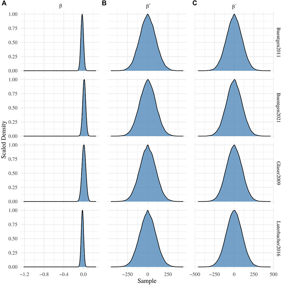
FIGURE 2. Posterior densities for the key regression model parameters. Each row contains the posterior densities for the model involving the temperature reconstruction indicated by the labels on the right of the plots. All densities have been scaled to a maximum of one. The (A) column contains the posterior densities for the baseline regression coefficient; the (B) column contains the posterior densities for the regression coefficient when the given temperature record is above the most likely upper threshold; and the (C) column contains the posterior densities for the regression coefficient when the given temperature record is below the most likely lower threshold. Note that the x-axis appears large in the left column only because the MCMC sampled and retained some low values for that parameter. While the densities in that column are largely normal and centred on zero, we nevertheless include the low values for the sake of transparency and reporting accuracy.

Importantly for the present study, the results indicate specifically that extreme temperatures had no discernible impact on conflict levels. The posterior distributions for the upper and lower extreme value regression coefficients were estimated to be zero on average, as noted above. They also had variances that reflected the relevant priors (Figure 2). This means that there was insufficient information in the data to update those prior distributions. The reason for this, computationally, was that the highest likelihood thresholds were outside the range of observed temperature deviations (Figure 3). The upper threshold was estimated to be higher than the highest observed temperature deviation in each reconstruction ($\sim 3\text{–}5$). Similarly, the lower threshold was estimated to be lower than the lowest observed temperature deviations (d∼6–15). Thus, the MCMC determined that the most likely parameter values effectively excluded thresholds—it pushed those thresholds beyond the observed data. This meant that no threshold effects (β⁺ and β⁻) could be estimated. Instead, the optimal solution was one in which temperature deviations had no effect on conflict over the whole range of observed temperature values.

FIGURE 3

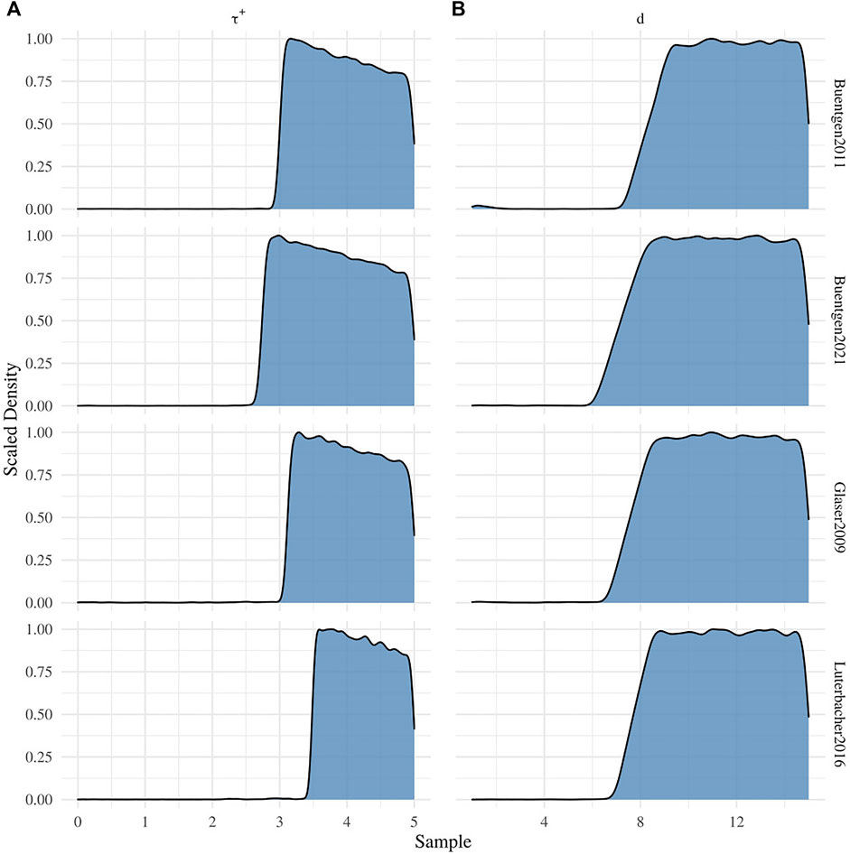
FIGURE 3. Posterior densities for the estimated temperature threshold values. Each row contains the posterior densities for the model involving the temperature reconstruction indicated by the labels on the right of the plots. All densities have been scaled to a maximum of one. The (A) column contains the posterior density estimates for the upper threshold value, and the (B) column contains the estimates for the difference between the upper and lower threshold.

Discussion and Conclusion

In HBO’s TV adaptation of the first novel in George R.R. Martin’s A Song of Ice and Fire series, King Robert says to his friend and advisor Ned Stark, “(t)here’s a war coming, Ned. I don’t know when, I don’t know who we’ll be fighting; but it’s coming.” These lines convey something about the nature of warfare: it appears to inevitably arise from some inexorable process that is difficult to predict. For at least 60 years, social scientists have tried to understand that process by identifying the correlates of warfare, motivated largely by a desire to predict and ideally prevent the process from giving rise to violence in the future (Suzuki et al., 1998). Recently, climate change has taken a central position in the literature on this topic, with many scholars declaring that climatic changes can be expected to increase the risk of violent conflict (e.g., Burke et al., 2009, 2015; Hsiang et al., 2013; Schmidt et al., 2021).

The results of the present study are not consistent with this claim. They indicate that even extreme climate conditions (as indicated by temperature reconstructions) did not affect conflict levels in Europe during the second millennium CE. This finding is perhaps surprising. Not only were there substantial climatic fluctuations in Europe during the second millennium CE, but also for much of the time period in question European societies were substantially less technologically developed than present-day European societies and were also more reliant on local agriculture. Less complex technology and greater dependence on local resources, one would think, should have made European societies susceptible to environmental shocks, especially large ones. But that does not seem to be the case. There is no evidence that the Little Ice Age or any of the other environmental shocks that impacted Europe during the second millennium CE affected conflict levels on average.

Why did our analysis fail to identify an impact of extreme climatic events on conflict levels in Europe during the second millennium CE? There are at least six explanations that are worth considering, some of which we alluded to earlier. The first three we think can be discounted by careful reasoning. The last three, however, are harder to eliminate at present and suggest avenues for future research.

The first explanation—one we think can be discounted—involves sampling biases in the conflict record. As explained earlier, the conflict data we analysed were compiled from authoritative conflict databases. But, since no historical database is likely to be complete, it is possible that the record we analysed is missing conflict events for several reasons. Not all conflicts that actually occurred were necessarily recorded, for example, and more recent periods are likely to be better represented because of document survival biases or other period-specific differences in reporting. Spatial gaps may be present in the data as well. Some sub-regions in western Europe may have been more important to historians and chroniclers, such as regions that were economically and politically important to ruling elites. In addition, the density of surviving historical documents varies spatially within Europe, with early historical coverage concentrated around major urban centers and in the south, particularly France and Italy. Thus, we should expect the Tol and Wanger (2010) conflict record to be incomplete and biased. However, there is reason to believe that regional-scale trends in second millennium conflict levels are likely captured by the Tol and Wagner (2010) record. Most major conflicts involved Europe’s largest, most literate societies. So, the most significant conflicts were probably recorded in a sufficient number of archives that knowledge of them survived to the present. This means that trends in economically and politically important conflicts are likely reflected in the record we analysed. There is also no obvious trend(s) in the record that might indicate a persistent document survival bias (Figure 1). Moreover, geographic unevenness would not be a significant problem for our analysis. If conflict levels were substantially affected by temperature variation in general, then we would expect the conflict records of any sizable sub-region within Europe to respond in the roughly same way to region-wide temperature changes.

Another potential explanation that we think can be discounted involves biases in the four temperature time-series. The temperature proxies we analysed are based on historical documents, tree-ring widths, or a combination of the two. Neither primary source is evenly distributed in space or time within Europe and, therefore, they undoubtedly contain biases. These biases will be acute for short term temperature fluctuations and sub-regions within western Europe. Recent research has also demonstrated that methodological and analytical choices involved in the production of tree-ring-based temperature reconstructions affect the patterns present in those reconstructions (Büntgen et al., 2021). Variability with respect to analytical choices of researchers—all of which may be justifiable—can lead to biases in and differences among individual reconstructions even when they are based on overlapping source data (some of the same trees or trees from the same regions). Despite these known biases, however, the reconstructions all appear to contain the same long-term, large-scale signal. They have each been shown to correlate positively with temperature variations during instrumental periods with Pearson’s R values ranging from 0.7 to 0.8. One of the reconstructions in particular—the one created by Büntgen et al. (2021)—averages out methodological differences and correlates very well (0.79, p < 0.001) with instrumental observations at different scales. It also has autocorrelation properties that match those of instrumental observations, and it has considerable predictive power for 20th and 21st century temperatures in the Northern Hemisphere. Taken together, the diagnostics performed by the scientists who produced the reconstructions appear to reflect their target reasonably well. Thus, despite their imperfections, the temperature time-series very likely capture regional trends and variations during the Common Era—this is especially true for the newest ensemble reconstruction produced by Büntgen et al. (2021). It is unlikely, then, that at the scale and resolution of our analysis, biases present in the temperature reconstructions account for our findings.

A third potential explanation, and the last we find unconvincing, is that we looked at the wrong type of climate data. The main agriculture staple in Europe throughout most of the second millennium was cereal grain (e.g., wheat, barley, rye, and oats) (Alfani and Ó Gráda, 2018; Ljungqvist et al., 2021). Yields for the main grain crops are affected by climate conditions, especially significant deviations from optimal conditions (Zscheischler et al., 2017). But, sensitivity to temperature specifically varies with crop type and region (Ljungqvist et al., 2021). Wheat, for example, is known to be quite tolerant of temperature deviations within the range of variation indicated by the reconstructions, even during much of the Little Ice Age (Porter and Gawith, 1999). In contrast, precipitation and, crucially, the timing of precipitation is very important for determining wheat yields (Brooks et al., 2018; Alfani, 2010). Thus, temperature may simply be the wrong covariate for investigating climate-conflict dynamics in Europe given that different crops react differently to temperature deviations. On its own, though, this explanation is wanting. Temperature variation is often used as a general climate indicator. The reason for this is that average temperatures (average over large areas and long spans of time) are associated with certain weather patterns and, so, major deviations in average temperatures are likely to entail changes in those patterns (Arnell et al., 2019). Extreme temperature deviations, therefore, could be expected to lead to significant changes in precipitation amounts and annual distributions of precipitation. Because both precipitation extremes—flooding on the one hand, and drought on the other—would have been bad for any cereal grain production, the temperature proxies we looked at should still be relevant. Essentially, the reconstructions we used can be thought of as general climate indicators and extreme values would likely have meant local, short-term disruptions to “normal” weather patterns. Crucially, the specific direction of that disruption with respect to precipitation—more rainfall or less—is not as important as the fact that a major disruption occurred. Substantial perturbations in either direction would likely have affected grain yields even though temperature may not have been the proximate cause (Zscheischler et al., 2017).

The fourth potential explanation—the first that we think is plausible—is that spatial aggregation of the data masked the true climate-conflict dynamics. This could occur in at least two ways. A change in temperature can lead to different effects in different locations (Mahlstein et al., 2013). A change in average European temperature may have produced different localised responses. Some areas might have been negatively affected while others were not. In fact, some research has indicated that northern and southern Europe will likely experience dramatically different outcomes as a result of continued global warming, with water shortages expected in the south and an increase in agricultural land in the north (e.g., Bindi and Olesen, 2011). A similar pattern of regional differentiation may have occurred in the past, meaning that northern and southern European societies may have experienced very different agro-economic effects from changes in average temperature (Alfani, 2010; Alfani and Ó Gráda, 2018). Consequently, spatially heterogeneous climate-conflict relationships may be obscured by the spatially aggregated data. Some areas may have experienced a higher level of conflict while others did not for a given change in regional average temperatures. In a related way, spatial aggregation of the conflict record may have masked the impact of climate on conflict levels. Prior to the First World War, conflicts often only involved two main groups. Potentially, combining these events into a single series makes it harder to adequately model the conflict generating process because not all groups included in the aggregate dataset were equally likely to engage in conflict with the other groups represented in the dataset. For example, France would have been less likely to go to war with Poland, in part because they share no borders. In aggregate, then, differences between the likelihood of conflicts between pairs of combatants could average out the impacts of climate, which were also spatially aggregated in our analysis. Essentially, the likelihood that any given pair—or “dyad”—would have actually engaged in violent conflict cannot be controlled for. A dyad approach has, for this reason, become common in research on modern international conflict and politics (Croco and Teo, 2005; Gleditsch et al., 2014; Schmidt et al., 2021). In a dyad study, the unit of analysis is conflict in a given time interval between specified pairs of potential combatants. That way, locally-specific climate effects can be compared to conflicts between groups where at least one of the groups is certainly affected by the given climate variable and the groups in question formed a plausible dyad in the first place.

The fifth potential explanation is that the model we used is too simplistic to account for climate–conflict dynamics. Climate-change driven resource shortages may be involved in conflict levels in more complex ways than can be evaluated with linear or even broken-stick models. Resource shortages, for example, could be both a cause and consequence of conflict. A crop shortfall could put additional pressure on a leader, affecting their decision-making vis-a-vis engaging in conflict. But at the same time, launching and sustaining conflicts consumes resources. In the Late Medieval period, it would not have been uncommon for bands of soldiers to extract resources from the area they happened to be moving through or positioned in (Howard, 2009; Alfani, 2010). With enough troops or a long enough campaign, the draw on local resources would have been significant. Even without bad weather, then, local shortages could arise as a consequence of conflict. Additionally, war often would have disrupted trade, which would remove a key resource buffer—local shortfalls could not be compensated by buying goods from elsewhere (Howard, 2009). In more recent periods, conflict still drained resources, but supplies were centrally coordinated rather than having soldiers simply pillage what they needed from locals. Nevertheless, conflict is costly and can draw down a society’s resources, increasing the risk of critical shortages with or without additional shocks from bad weather. This dynamic creates a feedback that could be hard to detect empirically even at an annual resolution and may require more complex statistical models. Along similar lines, it may be necessary to take into account additional mediating variables—e.g., population size, carrying capacity, political history—before the impact of climate change on conflict levels can be detected (Schmidt et al., 2021). Climate change including extreme events like the Little Ice Age may only impact conflict levels when a society is near its effective carrying capacity, which is a function of technology, population size, and the ability of socioeconomic institutions to buffer shortages (Alfani, 2010; Alfani and Ó Gráda, 2018). Without including interactions between these potential mediators and the climate covariate, the impact of climate change on conflict levels may be obscured by all of the other factors driving variation in the latter.

The final plausible possibility we have identified is that the scarcity mechanism may simply be insufficient for explaining long-term variations in conflict levels. This could be true irrespective of whether the scarcity is driven by average or extreme environmental conditions. Humans often fight for social, political, and economic reasons having little to do directly with resource shortages. The aforementioned Wars of the Roses are a prime example. The wars are generally thought to have erupted out of contentions over rival claims to the English throne (Hicks, 2012). Resources undoubtedly played a role, of course. In a sense, the throne is the ultimate resource (access to power, influence, and wealth) and resources were required to take it. But, the elite houses who wanted it had sufficient wealth that scarcity was unlikely to be a proximate motivating factor. If anything, engaging in the conflict over the crown created opportunity costs and resulted in financial losses, not to mention incurring the risk of imprisonment and death—“When you play the game of thrones, you win or die”, declared Cersei Lannister (Martin, 1996). Thus, while the crown was a prized, scarce resource, desire for it was not needs-based. Instead, actors fought for this resource out of greed, and it was largely insensitive to the weather—a drought or flood would not have changed the crown’s availability. A simple scarcity mechanism might, therefore, be insufficient to explain the conflicts, at least where “scarcity” refers only to crop yields or abstractly to economic resources.

We are left, then, with the puzzle we started with: How is it that significant climate changes apparently had no impact on second millennium CE European conflict incidence? The short answer, we think, may be that conflict happened mostly for other reasons, as we just explained. But, the other explanations we discussed above suggest a few avenues for future research. One of these is to examine the impact of other climate variables, such as rainfall. Another possibility is to look at additional mediating variables such as population size and political histories. A third avenue is to disaggregate the climate and conflict data into regional datasets. Lastly, future research could potentially involve more complex statistical models designed to include feedback between resources and conflict levels; computer simulations and purely mathematical models may be useful in this regard.

Even if climate change did have no impact on conflict incidence, it is worth highlighting that other dimensions of conflict may have been affected. The frequency of warfare is only one dimension of conflict within and between human groups. Others include conflict onset, duration, category, and magnitude. Each of these dimensions will be harder to evaluate than simple incidence. Onset and duration are probably the easiest to explore if precise start and end dates are available for each conflict. Evaluating different categories of conflict, say rebellion versus inter-state warfare, would involve more detailed historical research, but it may be possible to achieve a high level of confidence about the categorizations. Magnitude, unfortunately, would be much harder to measure for historical conflicts since any appropriate metric, like number of battle deaths, will probably be hard to estimate for pre-modern periods. Despite these potential challenges, though, research into the impact of climate change on these other dimensions of conflict over the long-term would be informative and important. If a relationship between climate change and one of these other dimensions was found, the fact that incidence appears to be unaffected would be less puzzling—such a finding would mean that intuitively appealing explanations like the scarcity mechanism may hold, just not in the most obvious way.

Despite not answering the question that motivated our study, our results have implications for our understanding of the impact of extreme events on society. Climatological extremes may have impacted societies in particular ways without those impacts reverberating to every potential domain. There is evidence, for instance, that the cold of the Little Ice Age was recognised as intense and anomalous by people who experienced it firsthand. The historical record contains references to water bodies freezing unexpectedly along with frequent mentions of crop failures, famines, and farms being deserted during this period (e.g., Holopainen and Helama, 2009; Alfani, 2010; Lockwood et al., 2017; Alfani and Ó Gráda, 2018; Athimon and Maanan, 2018). So, it seems safe to assume there were impacts. And yet our study has revealed that extreme temperature deviations had no clear impact on regional conflict levels. We can, therefore, infer that while extreme climate events likely did have some impact on European societies during the second millennium, the effects were circumscribed and contingent. An implication of this is that context matters in the analysis of the impact of extreme climatic events, possibly as much as the extreme nature of the events themselves. What makes a climatic event extreme for human societies may have more to do with its ultimate effects than its intrinsic character.

Data Availability Statement

The original contributions presented in the study are included in the article/Supplementary Material, further inquiries can be directed to the corresponding author.

Author Contributions

WC, MC, MS, and HG collectively conceived of the research and study design. WC and MS gathered the required data. WC developed the R code and ran the analyses. WC, MC, MS, and HG collectively interpreted the results. WC led the writing of this manuscript with contributions from MC, MS, and HG.

Funding

The Max Planck Society funds the independent Extreme Events Research Group who conducted this research. Canada Research Chairs Program (231256). Canada Foundation for Innovation (36801). British Columbia Knowledge Development Fund (962-805808). Simon Fraser University (no award number).

Conflict of Interest

The authors declare that the research was conducted in the absence of any commercial or financial relationships that could be construed as a potential conflict of interest.

Publisher’s Note

All claims expressed in this article are solely those of the authors and do not necessarily represent those of their affiliated organizations, or those of the publisher, the editors and the reviewers. Any product that may be evaluated in this article, or claim that may be made by its manufacturer, is not guaranteed or endorsed by the publisher.

Supplementary Material

The Supplementary Material for this article can be found online at: https://www.frontiersin.org/articles/10.3389/feart.2021.769107/full#supplementary-material

References

Adger, W. N., Pulhin, J. M., Barnett, J., Dabelko, G. D., Hovelsrud, G. K., Levy, M., et al. (2014). “Human Security,” in Climate Change 2014: Impacts, Adaptation, and Vulnerability: Working Group II Contribution to the Fifth Assessment Report of the Intergovernmental Panel on Climate Change. Editors C. Field, V. Barros, D. Dokken, K. Mach, M. Mastrandrea, T. Biliret al. (Cambridge University Press), 755–791.

Google Scholar

Alfani, G. (2010). Climate, Population and Famine in Northern italy: General Tendencies and Malthusian Crisis, Ca. 1450-1800. Ann. de Dèmographie Historique 120, 23–53. doi:10.3917/adh.120.0023

CrossRef Full Text | Google Scholar

Alfani, G., and Ó Gráda, C. (2018). The Timing and Causes of Famines in Europe. Nat. Sustain. 1, 283–288. doi:10.1038/s41893-018-0078-0

CrossRef Full Text | Google Scholar

Allen, M. W., Bettinger, R. L., Codding, B. F., Jones, T. L., and Schwitalla, A. W. (2016). Resource Scarcity Drives Lethal Aggression Among Prehistoric hunter-gatherers in central california. Proc. Natl. Acad. Sci. USA 113, 12120–12125. doi:10.1073/pnas.1607996113

PubMed Abstract | CrossRef Full Text | Google Scholar

Arnell, N. W., Lowe, J. A., Challinor, A. J., and Osborn, T. J. (2019). Global and Regional Impacts of Climate Change at Different Levels of Global Temperature Increase. Climatic Change 155, 377–391. doi:10.1007/s10584-019-02464-z

CrossRef Full Text | Google Scholar

Athimon, E., and Maanan, M. (2018). Vulnerability, Resilience and Adaptation of Societies during Major Extreme Storms during the Little Ice Age. Clim. Past 14, 1487–1497. doi:10.5194/cp-14-1487-2018

CrossRef Full Text | Google Scholar

Bindi, M., and Olesen, J. E. (2011). The Responses of Agriculture in Europe to Climate Change. Reg. Environ. Change 11, 151–158. doi:10.1007/s10113-010-0173-x

CrossRef Full Text | Google Scholar

Black, J. (2007). European Warfare in a Global Context, 1660-1815. London: Routledge, 1660–1815. doi:10.4324/9780203964828

CrossRef Full Text | Google Scholar

Brandt, P. T., Williams, J. T., Fordham, B. O., and Pollins, B. (2000). Dynamic Modeling for Persistent Event-Count Time Series. Am. J. Polit. Sci. 44, 823. doi:10.2307/2669284

CrossRef Full Text | Google Scholar

Buhaug, H. (2015). Climate-conflict Research: Some Reflections on the Way Forward. Wires Clim. Change 6, 269–275. doi:10.1002/wcc.336

CrossRef Full Text | Google Scholar

Büntgen, U., Allen, K., Anchukaitis, K. J., Arseneault, D., Boucher, É., Bräuning, A., et al. (2021). The Influence of Decision-Making in Tree Ring-Based Climate Reconstructions. Nat. Commun. 12, 3411. doi:10.1038/s41467-021-23627-6

PubMed Abstract | CrossRef Full Text | Google Scholar

Büntgen, U., Tegel, W., Nicolussi, K., McCormick, M., Frank, D., Trouet, V., et al. (2011). 2500 Years of European Climate Variability and Human Susceptibility. Science 331, 578–582. doi:10.1126/science.1197175

PubMed Abstract | CrossRef Full Text | Google Scholar

Burke, M. B., Miguel, E., Satyanath, S., Dykema, J. A., and Lobell, D. B. (2009). Warming Increases the Risk of Civil War in Africa. Proc. Natl. Acad. Sci. 106, 20670–20674. doi:10.1073/pnas.0907998106

CrossRef Full Text | Google Scholar

Burke, M., Hsiang, S. M., and Miguel, E. (2015). Climate and Conflict. Annu. Rev. Econ. 7, 577–617. doi:10.1146/annurev-economics-080614-115430

CrossRef Full Text | Google Scholar

Carleton, W. C., Campbell, D., and Collard, M. (2021). A Reassessment of the Impact of Temperature Change on European Conflict during the Second Millennium Ce Using a Bespoke Bayesian Time-Series Model. Climatic Change 165. doi:10.1007/s10584-021-03022-2

CrossRef Full Text | Google Scholar

Carleton, W. C., Campbell, D., and Collard, M. (2017). Increasing Temperature Exacerbated Classic Maya Conflict over the Long Term. Quat. Sci. Rev. 163, 209–218. doi:10.1016/j.quascirev.2017.02.022

CrossRef Full Text | Google Scholar

Collard, M., Carleton, W. C., and Campbell, D. A. (2021). Rainfall, Temperature, and Classic Maya Conflict: A Comparison of Hypotheses Using Bayesian Time-Series Analysis. PLOS ONE 16, e0253043. doi:10.1371/journal.pone.0253043

PubMed Abstract | CrossRef Full Text | Google Scholar

Croco, S. E., and Teo, T. K. (2005). Assessing the Dyadic Approach to Interstate Conflict Processes: A.k.a. "Dangerous" Dyad-Years. Conflict Management Peace Sci. 22, 5–18. doi:10.1080/07388940590915291

CrossRef Full Text | Google Scholar

Crowley, T. J., and Lowery, T. S. (2000). How Warm Was the Medieval Warm Period? AMBIO: A J. Hum. Environ. 29, 51–54. doi:10.1579/0044-7447-29.1.51

CrossRef Full Text | Google Scholar

D'Andrea, W. J., Huang, Y., Fritz, S. C., and Anderson, N. J. (2011). Abrupt Holocene Climate Change as an Important Factor for Human Migration in West greenland. Proc. Natl. Acad. Sci. 108, 9765–9769. doi:10.1073/pnas.1101708108

PubMed Abstract | CrossRef Full Text | Google Scholar

de Valpine, P., Paciorek, C., Turek, D., Michaud, N., Anderson-Bergman, C., Obermeyer, F., et al. (2021). NIMBLE User Manual. NIMBLE Development Team. doi:10.5281/zenodo.1211190

CrossRef Full Text | Google Scholar

DiPaolo, M. (2018). Fire and Snow: Climate Fiction from the Inklings to Game of Thrones. State University of New York Press.

Google Scholar

Feder, P. I. (1975). On Asymptotic Distribution Theory in Segmented Regression Problems–Identified Case. Ann. Stat., 49–83.

Google Scholar

F. Tallett, and D. J. B. Trim (Editors) (2010). “Then Was Then and Now Is Now’: An Overview of Change and Continuity in Late–Medieval and Early–Modern Warfare,” European Warfare, 1350–1750 (Cambridge University Press). doi:10.1017/CBO9780511806278

CrossRef Full Text | Google Scholar

Geweke, J. (1992). “Evaluating the Accuracy of Sampling-Based Approachesto the Calculation of Posterior Moments,” in Bayesian Stastistics. Editors J. M. Bernardo, J. O. Berger, A. P. Dawid, and A. F. M. Smith (Clarendon Press), 169–193.

Google Scholar

Glaser, R., and Riemann, D. (2009). A Thousand-Year Record of Temperature Variations for germany and central Europe Based on Documentary Data. J. Quat. Sci. 24, 437–449. doi:10.1002/jqs.1302

CrossRef Full Text | Google Scholar

Gleditsch, K. S., Metternich, N. W., and Ruggeri, A. (2014). Data and Progress in Peace and Conflict Research. J. Peace Res. 51, 301–314. doi:10.1177/0022343313496803

CrossRef Full Text | Google Scholar

Gleditsch, N. P., Wallensteen, P., Eriksson, M., Sollenberg, M., Strand, H., Collier, P., et al. (2002). Armed Conflict 1946–2001: A New Dataset. J. Peace Res. 3939.

Google Scholar

Glowacki, L., and Wrangham, R. W. (2013). The Role of Rewards in Motivating Participation in Simple Warfare. Hum. Nat. 24, 444–460. doi:10.1007/s12110-013-9178-8

PubMed Abstract | CrossRef Full Text | Google Scholar

Gornall, J., Betts, R., Burke, E., Clark, R., Camp, J., Willett, K., et al. (2010). Implications of Climate Change for Agricultural Productivity in the Early Twenty-First century. Phil. Trans. R. Soc. B 365, 2973–2989. doi:10.1098/rstb.2010.0158

PubMed Abstract | CrossRef Full Text | Google Scholar

Green, D. (2014). The Hundred Years War: A People’s History. Yale University Press.

Google Scholar

Hatfield, J. L., Dold, C., Brown, T. T., Hatfield, J. L., and Dold, C. (2018). Agroclimatology and Wheat Production: Coping with Climate Change. Front. Plant Sci. 9. doi:10.3389/fpls.2018.00224

PubMed Abstract | CrossRef Full Text | Google Scholar

Hicks, M. (2012). The Wars of the Roses. Yale University Press.

Google Scholar

High Representative of the European Union for Foreign Affairs and Security Policy (2013). Joint Communication to the European Parliament and the Council: The EU’s Comprehensive Approach to External Conflict and Crises. Tech. rep. Brussels: European Commission.

Google Scholar

Holopainen, J., and Helama, S. (2009). Little Ice Age Farming in Finland: Preindustrial Agriculture on the Edge of the Grim Reaper's Scythe. Hum. Ecol. 37, 213–225. doi:10.1007/s10745-009-9225-6

CrossRef Full Text | Google Scholar

Houweling, H. W., and Siccama, J. G. (1985). The Epidemiology of War, 1816-1980. J. Conflict Resolution 29, 641–663. doi:10.1177/0022002785029004007

CrossRef Full Text | Google Scholar

Howard, M. (2009). War in European History. Oxford University Press.

Google Scholar

Hsiang, S. M., Burke, M., and Miguel, E. (2013). Quantifying the Influence of Climate on Human Conflict. Science 341, 1235367. doi:10.1126/science.1235367

PubMed Abstract | CrossRef Full Text | Google Scholar

Kassambara, A. (2020). Ggpubr: ’ggplot2’ Based Publication Ready Plots. R package version 0.4.0.

Google Scholar

Kennett, D. J., Breitenbach, S. F. M., Aquino, V. V., Asmerom, Y., Awe, J., Baldini, J. U. L., et al. (2012). Development and Disintegration of Maya Political Systems in Response to Climate Change. Science 338, 788–791. doi:10.1126/science.1226299

PubMed Abstract | CrossRef Full Text | Google Scholar

Koubi, V. (2019). Climate Change and Conflict. Annu. Rev. Polit. Sci. 22, 343–360. doi:10.1146/annurev-polisci-050317-070830

CrossRef Full Text | Google Scholar

Ljungqvist, F. C., Seim, A., and Huhtamaa, H. (2021). Climate and Society in European History. Wires Clim. Change 12. doi:10.1002/wcc.691

CrossRef Full Text | Google Scholar

Lockwood, M., Owens, M., Hawkins, E., Jones, G. S., and Usoskin, I. (2017). Frost Fairs, Sunspots and the Little Ice Age. Astron. Geophys. 58, 17–223. doi:10.1093/astrogeo/atx057

CrossRef Full Text | Google Scholar

Luterbacher, J., Werner, J. P., Smerdon, J. E., Fernández-Donado, L., González-Rouco, F. J., Barriopedro, D., et al. (2016). European Summer Temperatures since Roman Times. Environ. Res. Lett. 11, 024001. doi:10.1088/1748-9326/11/2/024001

CrossRef Full Text | Google Scholar

Mach, K. J., Kraan, C. M., Adger, W. N., Buhaug, H., Burke, M., Fearon, J. D., et al. (2019). Climate as a Risk Factor for Armed Conflict. Nature 571, 193–197. doi:10.1038/s41586-019-1300-6

PubMed Abstract | CrossRef Full Text | Google Scholar

Mahlstein, I., Daniel, J. S., and Solomon, S. (2013). Pace of Shifts in Climate Regions Increases with Global Temperature. Nat. Clim Change 3, 739–743. doi:10.1038/NCLIMATE1876

CrossRef Full Text | Google Scholar

Mann, M. E., Zhang, Z., Rutherford, S., Bradley, R. S., Hughes, M. K., Shindell, D., et al. (2009). Global Signatures and Dynamical Origins of the Little Ice Age and Medieval Climate Anomaly. Science 326, 1256–1260. doi:10.1126/science.1177303

PubMed Abstract | CrossRef Full Text | Google Scholar

Martin, G. R. (1996). A Game Of Thrones. US: Bantam Spectra.

Google Scholar

Neiberg, M. S. (2003). Warfare and Society in Europe. London: Routledge. doi:10.4324/9780203643525

CrossRef Full Text | Google Scholar

Porter, J. R., and Gawith, M. (1999). Temperatures and the Growth and Development of Wheat: A Review. Eur. J. Agron. 10, 23–36. doi:10.1016/S1161-0301(98)00047-1

CrossRef Full Text | Google Scholar

R Core Team (2021). R: A Language and Environment for Statistical Computing. Vienna, Austria: R Foundation for Statistical Computing.

Google Scholar

Richardson, L. F. (1944). The Distribution of Wars in Time. J. R. Stat. Soc. 107, 242–250. doi:10.2307/2981216

CrossRef Full Text | Google Scholar

Schmidt, C. J., Lee, B. K., and Mitchell, S. M. (2021). Climate Bones of Contention: How Climate Variability Influences Territorial, Maritime, and River Interstate Conflicts. J. Peace Res. 58, 132–150. doi:10.1177/0022343320973738

CrossRef Full Text | Google Scholar

Suzuki, S., Krause, V., and Singer, J. (1998). The Correlates of War Project: A Bibliographic History of Scientific Study of War and Peace, 1964-2000. Conflict Management Peace Sci. 19, 69–107.

Google Scholar

Theisen, O. M. (2012). Climate Clashes? Weather Variability, Land Pressure, and Organized Violence in kenya, 1989-2004. J. Peace Res. 49, 81–96. doi:10.1177/0022343311425842

CrossRef Full Text | Google Scholar

Tol, R. S. J., and Wagner, S. (2010). Climate Change and Violent Conflict in Europe over the Last Millennium. Climatic Change 99, 65–79. doi:10.1007/s10584-009-9659-2

CrossRef Full Text | Google Scholar

Turney, C. S. M., McGregor, H. V., Francus, P., Abram, N., Evans, M. N., Goosse, H., et al. (2019). Introduction to the Special Issue "Climate of the Past 2000 years: Regional and Trans-regional Syntheses". Clim. Past 15, 611–615. doi:10.5194/cp-15-611-2019

CrossRef Full Text | Google Scholar

US Department of Defense (2010). Quadrennial Defense Review Report 2010. Defense. doi:10.1017/CBO9781107415324.004

CrossRef Full Text | Google Scholar

Vasseur, D. A., and Yodzis, P. (2004). The Color of Environmental Noise. Ecology 85, 1146–1152. doi:10.1890/02-3122

CrossRef Full Text | Google Scholar

Von Uexkull, N., Croicu, M., Fjelde, H., and Buhaug, H. (2016). Civil Conflict Sensitivity to Growing-Season Drought. Proc. Natl. Acad. Sci. USA 113, 12391–12396. doi:10.1073/pnas.1607542113

PubMed Abstract | CrossRef Full Text | Google Scholar

Wickham, H. (2016). ggplot2: Elegant Graphics for Data Analysis. Verlag, NY: Springer.

Google Scholar

Zhang, D. D., Jim, C. Y., Lin, G. C.-S., He, Y.-Q., Wang, J. J., Lee, H. F., et al. (2006). Climatic Change, Wars and Dynastic Cycles in china over the Last Millennium. Climatic Change 76, 459–477. doi:10.1007/s10584-005-9024-z

CrossRef Full Text | Google Scholar

Zscheischler, J., Orth, R., and Seneviratne, S. I. (2017). Bivariate Return Periods of Temperature and Precipitation Explain a Large Fraction of European Crop Yields. Biogeosciences 14, 3309–3320. doi:10.5194/bg-14-3309-2017

CrossRef Full Text | Google Scholar