Numerical Simulation Study of Tracking the Displacement Fronts and Enhancing Oil Recovery Based on Ferrofluid Flooding

Water flooding is crucial means to improve oil recovery after primary production. However, the utilization ratio of injected water is often seriously affected by heterogeneities in the reservoir. Identification of the location of the displacement fronts and the associated reservoir heterogeneity is important for the management and improvement of water flooding. In recent years, ferrofluids have generated much interest from the oil industry owning to its unique properties. First, saturation of ferrofluids alters the magnetic permeability of the porous medium, which means that the presence of ferrofluids should produce magnetic anomalies in an externally imposed magnetic field or the local geomagnetic field. Second, with a strong external magnetic field, ferrofluids can be guided into regions that were bypassed and with high residual oil saturation. In view of these properties, a potential dual-application of ferrofluid as both a tracer to locate the displacement front and a displacing fluid to improve recovery in a heterogeneous reservoir is examined in this paper. Throughout the injection process, the magnetic field generated by electromagnets and altered by the distribution of ferrofluids was calculated dynamically by applying a finite element method, and a finite volume method was used to solve the multiphase flow. Numerical simulation results indicate that the displacement fronts in reservoirs can indeed be detected, through which the major features of reservoir heterogeneity can be inferred. After the locations of the displacement fronts and reservoir heterogeneities are identified, strong magnetic fields were applied to direct ferrofluids into poorly swept regions and the efficiency of the flooding was significantly improved.

Introduction

Ferrofluids are stable colloids composed of small nano-scale solid, magnetic particles coated with a molecular layer of dispersant and suspended in a liquid carrier (Rosensweig, 1997). Thermal agitation keeps the particles suspended, and the coatings prevent the particles from coagulation. Its behavior and property can be controlled and changed by the magnetic field (Odenbach, 2008). Therefore, ferrofluid has many industrial applications, such as dynamic sealing, inertial and viscous damper, magnetic drug targeting, liquid microrobots, and so on (Raj and Moskowitz, 1990; Hou et al., 1999; Scherer and Figueiredo, 2005; Fan et al., 2020).

In the past years, ferrofluid flow in porous media has been the subject of various experimental and numerical studies. Borglin, Moridis, and Oldenburg et al. investigated the flow behavior of ferrofluid in porous media, the results showed that the effect of an external magnetic field on the flow of a ferrofluid in porous media is equivalent to the imposition of a magnetic body force, which means the flow of ferrofluids can be guided (Moridis et al., 1998; Oldenburg and Moridis, 1998; Borglin et al., 2000; Oldenburg et al., 2000). The above works, however, did not consider the impact of the ferrofluid on the magnetic field. The presence of ferrofluids should produce anomalies in the magnetic field because these fluids alter the magnetic permeability. Such anomalies, in principle, can be detected by magnetic anomaly detectors. Based on this feature, Sengupta (Sengupta, 2012) proposed an innovative approach to determining the fracture length and width by injecting ferrofluids into the fracture. When applying an external magnetic field, the ferrofluids in the fracture shall generate a secondary magnetic field which will have a definite phase difference from the original magnetic field. Once the phase difference is detected and processed by software an accurate representation of fractures can be made. Schmidt (Schmidt and Tour, 2012) proposed methods for magnetic imaging of geological structures, the principle is similar to Sengupta. Rahmani et al. used a ferrofluid slug to track the movement of a flooding front and studied reservoir permeability heterogeneity (Rahmani et al., 2014; Rahmani et al., 2015).

Water flooding, as is well recognized, is an effective approach to maintain reservoir pressure and improve oil recovery. However, heterogeneities or fractures present in China’s continental reservoirs can significantly decrease the sweep efficiency, leading to poor utilization ratios and low oil recovery. There is still a great potential to enhance the recovery (Han, 1995; Yu, 2000; Han, 2007; Yang, 2009; Han 2010). Therefore, it is urgent to find new oil displacement technology and method to overcome the problem of low oil displacement efficiency caused by reservoir heterogeneity and complex structure. In this paper, we study the potential of using ferrofluid both as a tracer and controllable displacing fluid during the whole flooding process. First, since the superparamagnetic nanoparticles in the ferrofluid can change the magnetic permeability of the flooded region, we study the magnetic anomalies and indicate the locations of displacement fronts, as shown in Figure 1A. And then as a displacing fluid that, guided by strong magnetic fields, can overcome reservoir heterogeneities and improve sweep efficiency and oil recovery, as shown in Figure 1B.

FIGURE 1

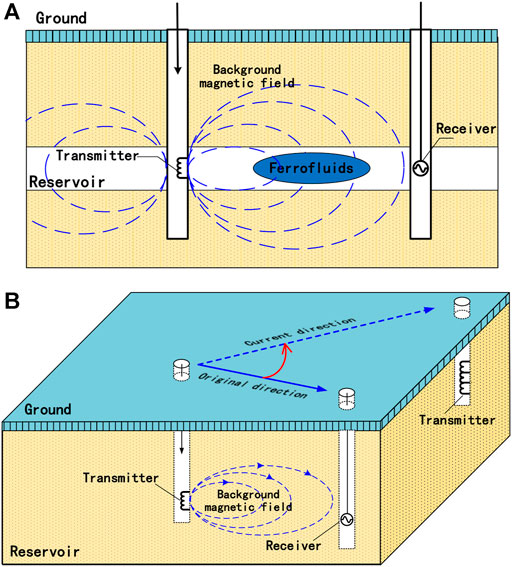
FIGURE 1. Schematic diagram of ferrofluid flooding technology: (A) Displacement front monitoring and tracking; (B) Displacement direction guiding and controlling.

Computational Methodology

Magnetic Field Calculation

In a quasi-static magnetic problem, the relations between the magnetic field strength $\mathbf{H}$, the magnetic flux density $\mathbf{B}$, the current density $\mathbf{J}$, and the magnetization $\mathbf{M}$ are given by Maxwell equations and the magnetic properties of the material of concern:

$\nabla \times \mathbf{H}=\mathbf{J}(1)$

$\nabla \cdot \mathbf{B}=0(2)$

$\mathbf{B}={\mu }_0\left(\mathbf{H}+\mathbf{M}\right)(3)$

Where ${\mu }_0$ is the permeability of vacuum.

Introducing the vector potential $\mathbf{A}$, which is defined by:

$\mathbf{B}=\nabla \times \mathbf{A}(4)$

with the additional assumption that $\nabla \cdot \mathbf{A}=0$, considering Eqs 3–5 can be transformed into

$\nabla \times \left(\frac{1}{{\mu }_0}\nabla \times \mathbf{A}-\mathbf{M}\right)=\mathbf{J}(5)$

In order to solve the differential Eq. 5, it is formulated into a boundary value problem by using the energy functional (Silvester and K. Chari, 1970; Kamminga, 1975)

$I={\displaystyle \underset{\Omega }{\int }\left(\frac{1}{{\mu }_0}{\displaystyle \int \mathbf{B}\cdot d\mathbf{B}-{\displaystyle \int \mathbf{M}\cdot d\mathbf{B}-\mathbf{J}\cdot \mathbf{A}}}\right)}dV(6)$

where $\Omega$ is the area of the region of study.

The variation $\delta I$ caused by a small variation of $\delta \mathbf{A}$ is equal to

$\delta I={\displaystyle \underset{\Omega }{\int }\left(1/{\mu }_0\mathbf{B}\cdot \delta \mathbf{B}-\mathbf{M}\cdot \delta \mathbf{B}\right)}dV-{\displaystyle \underset{\Omega }{\int }\mathbf{J}}\cdot \delta \mathbf{A}dV(7)$

Since the energy functional is stationary to any small variation in $\mathbf{A}$, the variation $\delta I$ must be zero, which gives

${\displaystyle \underset{\Omega }{\int }\left(1/{\mu }_0\mathbf{B}\cdot \delta \mathbf{B}-\mathbf{M}\cdot \delta \mathbf{B}\right)}dV-{\displaystyle \underset{\Omega }{\int }\mathbf{J}}\cdot \delta \mathbf{A}dV=0(8)$

In regions occupied by a ferrofluid, the magnetic solid particles in the ferrofluid become polarized with the imposition of an external magnetic field, and the ferrofluid is said to be “magnetized.” In this paper, we considered a water-based ferrofluid Hinano-FFW provided by a nanomaterials company in China. Although the composition of the fluid was not revealed, the magnetization curve of the fluid was provided to us. Ferrofluid magnetization curves are generally approximated by simple two-parameter arctan functions of the form (Oldenburg et al., 2000):

$M_{\text{ff}}=\alpha \times \arctan \left(\beta \times H\right)(9)$

where the subscript $\text{ff}$ stands for ferrofluid. For our particular fluid, $\alpha$ = 1×10⁴, $\beta$ = 3.5 × 10^–5.

Considering a permanent magnet, and the magnetization ${\mathbf{M}}_{\text{m}}$ can be defined by:

${\mathbf{M}}_{\text{m}}=M_{\text{m}}\sin {\alpha }_{\text{m}}\cos {\beta }_{\text{m}}\mathbf{i}+M_{\text{m}}\sin {\alpha }_{\text{m}}\sin {\beta }_{\text{m}}\mathbf{j}+M_{\text{m}}\cos {\alpha }_{\text{m}}\mathbf{k}(10)$

Where $M_{\text{m}}$ is the residual magnetization of a permanent magnet, ${\alpha }_{\text{m}}$ is the angle between the direction of the magnetization of the permanent magnet and the positive direction of the $z$ axis, ${\beta }_{\text{m}}$ is the angle between the direction of the magnetization of the permanent magnet and the positive direction of the $x$ axis, as shown in Figure 2.

FIGURE 2

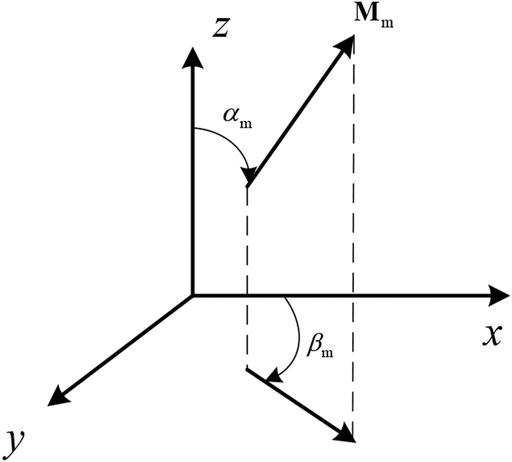
FIGURE 2. Diagram of the magnetization direction of permanent magnet.

In this paper, we consider the 2-D problem and the quasi-static magnetic problem solved by the finite element method. The magnetization ${\mathbf{M}}_{\text{m}}$ of a permanent magnet can be simplified:

${\mathbf{M}}_{\text{m}}=M_{\text{m}}\sin {\alpha }_{\text{m}}\cos {\beta }_{\text{m}}\mathbf{i}+M_{\text{m}}\sin {\alpha }_{\text{m}}\sin {\beta }_{\text{m}}\mathbf{j}(11)$

Thus, the magnetization term $\mathbf{M}$ in the Eq. 8 consists of two parts:

$\mathbf{M}={\mathbf{M}}_{\text{ff}}+{\mathbf{M}}_{\text{m}}(12)$

The computational region $\Omega$ was discretized by triangular grids. The current density $\mathbf{J}$ and the vector potential $\mathbf{A}$ only have component in $z$ direction:

$\mathbf{A}=\left(0,0,A\right),\mathbf{J}=\left(0,0,J\right)(13)$

From the requirement that the energy functional takes a stationary value, a set of $n$ equations are obtained:

$\frac{\partial I}{\partial A_i}\left(A_1,\dots ,A_n\right)=0,i=1,\dots ,n(14)$

where $n$ is the number of grid point.

Substituting Eqs 8, 9, 11, 12 into Eq. 14, we obtain Eq. 15 as follows:

$\begin{array}{l}{\displaystyle \underset{\Omega }{\int }\frac{1}{{\mu }_0}\left(B_x\frac{\partial B_x}{\partial A_i}+B_y\frac{\partial B_y}{\partial A_i}\right)}dV-{\displaystyle \underset{\Omega }{\int }\left(M_{\text{m}}\sin {\alpha }_{\text{m}}\cos {\beta }_{\text{m}}\frac{\partial B_x}{\partial A_i}+M_{\text{m}}\sin {\alpha }_{\text{m}}\sin {\beta }_{\text{m}}\frac{\partial B_y}{\partial A_i}\right)}dV-{\displaystyle \underset{\Omega }{\int }[\alpha \arctan \left(\frac{\beta }{{\mu }_0}{B}_x\right)\frac{\partial B_x}{\partial A_i}+}\alpha \arctan \left(\frac{\beta }{{\mu }_0}{B}_y\right)\frac{\partial B_y}{\partial A_i}]dV-{\displaystyle \underset{\Omega }{\int }J\frac{\partial A}{\partial A_i}}dV=\text{0}\end{array}(15)$

The potential in the k-th triangular element is assumed to be equal to

$A^k=\frac{1}{2{\Delta }^k}{\displaystyle \sum _i\left(a_i+b_{i}x+r_{i}y\right)A_i},i=\mathrm{1,2,3}(16)$

where ${\Delta }^k$ is the volume of k-th element, $A_i$ is the potential at the element’s vertex, $a_i$,$b_i$,$r_i$ are the coefficients associated with the element’s vertex positions $x_i$,$y_i$:

$\begin{array}{l}{a}_1=x_2{y}_3-x_3{y}_2,b_1=y_2-y_3,r_1=x_3-x_2\\ a_2=x_3{y}_1-x_1{y}_3,b_2=y_3-y_1,r_1=x_1-x_3\\ a_3=x_1{y}_2-x_2{y}_1,b_3=y_1-y_2,r_1=x_2-x_1\end{array}(17)$

Because the magnetic flux density $\mathbf{B}=\nabla \times \mathbf{A}$, considering Eq. 16, the components of magnetic induction can be obtained:

$B_x^k=\frac{1}{2{\Delta }^k}{\displaystyle \sum _i{r}_i{A}_i},B_y^k=-\frac{1}{2{\Delta }^k}{\displaystyle \sum _i{b}_i{A}_i}(18)$

Take the Eqs 16, 18 into Eq. 15, we can obtain a set of nonlinear equations:

$F_q\left(A_1,\dots ,A_n\right)=0,q=1,\dots ,n(19)$

and the solution was obtained by using the Newton-Raphson iterative method. Once the vector potential $\mathbf{A}$ was obtained, one can calculate the magnetic flux density by $\mathbf{B}=\nabla \times \mathbf{A}$.

Simulation of Ferrofluid Flowing in Porous Media

The magnetization of bulk ferrofluid increases with increasing external magnetic field strength, following Eq. 9. In the case of immiscible two-phase flows in porous media, and additional assumption that magnetization increases linearly with ferrofluid’s saturation was given by:

$M\left(S_{\text{ff}}\right)=M\left(S_{\text{ff}}=1\right)S_{\text{ff}}(20)$

When an external magnetic field is applied, the ferrofluid receives a magnetic body force ${\mathbf{F}}_m={\mu }_{0}M\nabla H$. This additional magnetic force term is added to the multiphase Darcy’s Equation (Oldenburg et al., 2000):

${\mathbf{v}}_{\text{ff}}=-\frac{k_{r\text{ff}}}{{\mu }_{\text{ff}}}\mathbf{k}\cdot \left(\nabla p_{\text{ff}}-{\rho }_{\text{ff}}g\nabla D-{\mu }_{0}M\nabla H\right)(21)$

where $\mathbf{k}=(k_x,k_y,k_z)$ is the permeability tensor, $k_r$ is the relative permeability, $\mu$ is fluid viscosity, $p$ is the fluid pressure, $\rho$ is the fluid density, and $D$ denotes the depth which is positive on the upward side, $g$ is the gravitational acceleration.

For simplicity, we considered the flow as isothermal and incompressible. Such simplifications are common in the analysis of water flooding. From the law of mass conservation, we know that a fluid in a control volume should meet:

${\displaystyle {\int }_{\partial V}-\left({\rho }_{\beta }{\mathbf{v}}_{\beta }\right)}\cdot \mathbf{n}dA+{\displaystyle {\int }_V{q}_{\text{m}\beta }}dV={\displaystyle {\int }_V\frac{\partial }{\partial t}}\left({\rho }_{\beta }\varphi S_{\beta }\right)dV(22)$

where the subscript $\beta =\left(\text{o, w, ff}\right)$ distinguishes the fluid, $\mathbf{n}$ is the outward normal unit vector of region boundary $\partial V$, $q_{\mathbf{m}\beta }$ is the source term that represents mass change per unit time and unit volume, $\varphi$ is the porosity.

Using a finite volume method to discretize the mass conservation equation, and the discrete nonlinear equation was also solved by using the Newton-Raphson iterative method.

Examples and Discussions

Tracking the Displacement Fonts of Ferrofluid Flooding

The first example that we considered is a horizontal porous media model as shown in Figure 3A, the left and right boundary is injector and producer, respectively. We assumed the top and bottom of porous media are closed boundaries. This model can be used to approximate flooding with a line drive pattern. The porosity is 0.2 and the permeability is 100 mD(10⁻³ μm²). A tiny permanent magnet was placed on the left side of porous media to generate a background magnetic field, the dimension is 2 cm × 4 cm and the residual flux density of the magnet is 1.19T, the background magnetic field is shown in Figure 3B.

FIGURE 3

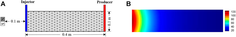
FIGURE 3. Simple porous media model. (A) Model geometry; (B) Distribution of background magnetic flux density norm |B| in units of Gs.

In the beginning, the model was saturated with oil, and the oil viscosity equals 5 mPa∙s and the density equal 850 kg/m³. Then we used ferrofluid to flooding this porous media, viscosity and density of ferrofluid are 3 mPa∙s and 1,187 kg/m³, respectively. The relative permeability of the ferrofluid phase $k_{r\text{ff}}=S_{\text{ff}}^2$. The relative permeability of the oil phase $k_{r\text{o}}={(1-S_{\text{ff}})}^2$. Both injection and production rates were set to 0.01 V_p/min, where V_p is the total pore volume. Since a week magnetic field generated by a tiny magnet, we assumed the magnetic force generated on the ferrofluid was neglected in this case.

The magnetic anomaly is defined as:

${\left|\mathbf{B}\right|}_{\text{anomaly}}=\frac{{\left|\mathbf{B}\right|}_{\text{current}}-{\left|\mathbf{B}\right|}_{\text{background}}}{{\left|\mathbf{B}\right|}_{\text{background}}}(\%)(23)$

where ${\left|\mathbf{B}\right|}_{\text{current}}$ is the norm magnetic flux density during ferrofluid flooding, and ${\left|\mathbf{B}\right|}_{\text{background}}$ is the normal of the magnetic flux density provided by the magnet before the ferrofluid flooding starts.

As Figure 4 shown, the distribution of magnetic anomalies is basically consistent with the ferrofluid saturation distribution. Near the injector is a high magnetic anomalous area because of the highest ferrofluid saturation, however, the decrease of ferrofluid saturation from the injector to the displacement font leads to a magnetic anomaly decrease.

FIGURE 4

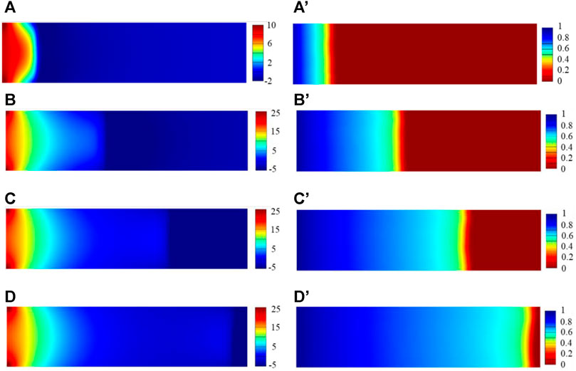
FIGURE 4. The ferrofluid saturation and magnetic anomaly distribution of numerical simulation at different time. (A–D) respectively show the magnetic anomaly at 10, 30, 50, 70 min; (A′-D′) respectively show the saturation distribution at 10, 30, 50, 70 min.

Figure 5 shows the ferrofluid saturation and magnetic anomaly curves from the left side to the right side of the porous media at several flooding periods. Note that the inflection point of each anomaly curve basically corresponds to the displacement fonts. For example, point 1 and point 2 of the anomaly curve at 30 min in Figure 5A, correspond to point 1 and point 2 of the saturation curve at 30 min in Figure 5B. It is worth noting that the area between these two points is exactly the displacement front. Thus, this remarkable fact indicates that one can track the ferrofluid fonts based on the magnetic anomaly information at every displacement stage.

FIGURE 5

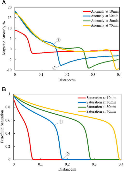
FIGURE 5. The ferrofluid saturation and magnetic anomaly curves along the porous media at 10, 30, 50,70 min. (A) Magnetic anomaly curves; (B) Saturation curves.

Evaluation of the Major Features of Reservoir Heterogeneity

It can be seen from the above section, that the ferrofluid displacement front can be tracked by capturing magnetic anomalies. Furthermore, the flow path of the ferrofluid can be obtained from the displacement front position, thus, the major geological characteristics of the reservoir can be inferred.

Consider a five-spot heterogeneous reservoir as Figure 6A shows, the reservoir size is 100 m × 100 m. The heterogeneous reservoir is divided into four regions with an injection well in the center and a production well at each of the four corners. The injection and production rates were set to 0.01 V_p/day. Assuming the reservoir has a porosity of 0.2, the permeability in region 1 is k₁ = 200 mD, and the permeability in regions 2, 3 and 4 is k₂ = k₃ = k₄ = 100 mD. In particular, the second region contains an elliptical low-permeability zone while the fourth region contains an elliptical high-permeability zone. The permeability of the two elliptical zones is 10 and 500 mD, respectively. In the beginning, the model was saturated with oil, and the fluid properties are the same as mentioned above. In order to provide a background magnetic field, an electromagnet EM was placed. The size of EM is 10 m × 0.4 m and the current intensity of EM is 10⁵ A/m². The background magnetic field is shown in Figure 6B.

FIGURE 6

FIGURE 6. A five-spot heterogeneous reservoir model. (A) Model geometry; (B) Distribution of background magnetic flux density norm log₁₀|B| in units of Gs.

As shown in Figure 7, due to the relatively high permeability of region 1 and region 4, the injected ferrofluid propagates faster in these areas, resulting in larger magnetic anomalies. On the contrary, the magnetic anomalies in region 2 and region 3 are relatively small. In particular, the magnetic anomaly in region 4 presents a fingering phenomenon. This is because there is a high permeability elliptical zone in region 4, which makes the injected ferrofluid flow to the production well faster than the other regions. So that the ferrofluid saturation is high at the same time, and resulting in a large magnetic anomaly. However, because the presence of the low permeability elliptical zone in region 2 blocks the flow of ferrofluid to the production well, the ferrofluid in region 2 has a small spread range and low saturation, so the magnetic anomalies are small. In the same way, the lower overall permeability of region 3 is also the reason for the smaller magnetic anomalies.

FIGURE 7

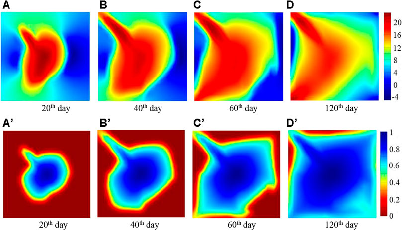
FIGURE 7. The magnetic anomaly and ferrofluid saturation distribution at different time. (A–D) respectively show the magnetic anomaly at 20th, 40th, 60th, 120th day; (A′–D′) respectively show the ferrofluid saturation at 20th, 40th, 60th, 120th day.

As shown in Figure 8, from the magnetic anomaly curves of production wells in different reservoir regions (star mark in Figure 6A), it can be seen that: 1) In the early stage of production, the magnetic anomalies of production well 1, 4 increased and decreased in production well 2, 3. This phenomenon indicates that the injected ferrofluid flows faster in regions 1, 4 than in regions 2, 3, and reflecting indirectly that the permeability of regions 1, 4 is higher than regions 2, 3; 2) Each magnetic anomaly curve has a rapidly rising time point, which corresponds to the moment when the ferrofluid flows into the production well; 3) Because the distribution of magnetic anomalies reflects the distribution of ferrofluid saturation, the magnetic anomaly change information can be used to analyze the flooding process in the reservoir, and so as to recognize the heterogeneous characteristics of the reservoir in general.

FIGURE 8

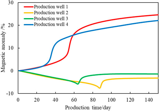
FIGURE 8. Magnetic anomaly curves of production well in different reservoir regions.

Monitoring-Controlling Integrated Ferrofluid Flooding Technology

From the above studies, it can be inferred that the ferrofluid flooding process can be monitored through the magnetic anomaly information, while the major heterogeneity characteristics of the reservoir can be recognized according to the flooding status. In addition, when there is an external magnetic field, the ferrofluid receives a magnetic force, and its flow behavior can be controlled by the magnetic force.

Consider a heterogeneous reservoir as Figure 9A shows. Assuming the reservoir has a porosity of 0.25, and the permeability is 500 mD. In particular, the reservoir contains two elliptical high-permeability zones. The permeability of the two elliptical zones is both 1,500 mD. In order to generate magnetic anomalies during the flooding process, an electromagnet EM1 is placed near the eastern part of the reservoir to provide a background magnetic field. The electromagnet EM1 with a size of 5 m × 0.4 m and a current density of 10⁵ A/m². The background magnetic field is shown in Figure 9B. It is worth noting that the background magnetic field is a weak magnetic field, and the generated magnetic force in ferrofluid is very small. So that its influence on the flooding can be ignored. The reservoir is initially saturated with oil, and ferrofluid is used to displace the reservoir. The fluid properties are the same as mentioned above. The injection and production rates were set to 0.025 V_p/day.

FIGURE 9

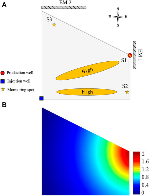
FIGURE 9. A heterogeneous reservoir model. (A) Model geometry; (B) Distribution of background magnetic flux density norm log₁₀|B| in units of Gs.

As the high-permeability zone is the dominant channel for flow, the injected ferrofluid mainly flows along the high-permeability zone, so the swept areas are mainly concentrated in the central and southern parts of the reservoir. When the 1.5V_p ferrofluid was injected, the oil in the central and southern areas of the reservoir was almost completely displaced, but the oil in the northern area of the reservoir was not displaced, as shown in Figures 10A–D.

FIGURE 10

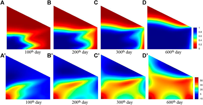
FIGURE 10. The ferrofluid saturation and magnetic anomaly distribution at different time. (A–D) respectively show the ferrofluid saturation at 100th, 200th, 300th, 600th day; (A′–D′) respectively show the magnetic anomaly at 100th, 200th, 300th, 600th day.

The distribution of magnetic anomalies in Figures 10A′–D′ shows: 1) At the early stage of flooding, the magnetic anomaly in the central region of the reservoir is relatively large, while the magnetic anomalies in the eastern and northern region of the reservoir are small; 2) At the middle stage of flooding, the magnetic anomaly in the central region of the reservoir is relatively large. These areas gradually increase and spread to the northern region of the reservoir; 3) At the later stage of flooding, the magnetic anomaly in the central and southern regions of the reservoir are generally large, while the magnetic anomaly in the northern region is still low.

From the analysis of the magnetic anomaly changes in the entire flooding process, it can be known that due to the existence of the high permeability zone, the injected ferrofluid is mainly displaced in the central and southern parts of the reservoir, so that the saturation of the ferrofluid is larger, and the magnetic anomaly is larger.

Figure 11 shows the magnetic anomaly curves of different monitoring spots in the reservoir, and the positions of the monitoring spots are shown in Figure 9A (star mark). It can be seen from the curves that the ferrofluid mainly flows to the production well and the eastern part of the reservoir because of the existence of the high permeability zone. Therefore, the magnetic anomaly curve of S1 and S2 which is located in the production well and the eastern part of the reservoir gradually increases with the flooding process, while the magnetic anomaly curve of S3 which is located in the northern part of the reservoir basically remains unchanged.

FIGURE 11

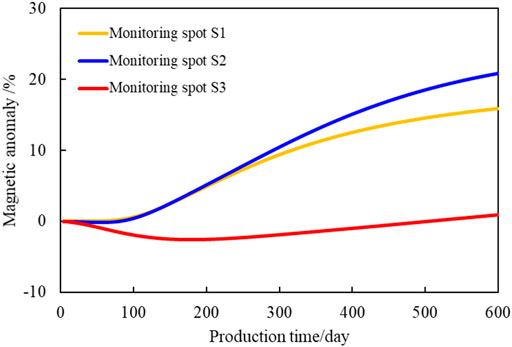
FIGURE 11. Magnetic anomaly curves of monitoring spots located in different region.

The magnetic anomaly curves of the three monitoring spots show that the injected ferrofluid is more inclined to flood the central and southern areas of the reservoir. Thus, there may be a “dominant flow channel" in this area. The northern part of the reservoir has not been affected, and there is still remaining oil in this area, which is the key area for development.

According to the analysis of the above magnetic anomaly curves, it can be seen that the ferrofluid displacement is mainly in the central and eastern parts of the oil reservoir. Therefore, the electromagnet EM2 is deployed near the northern part of the reservoir from the 120th day, and the strong magnetic field generated by EM2 is used to apply a huge magnetic field force on the ferrofluid, leading the ferrofluid to displace to the northern part of the reservoir. The electromagnet EM2 with a size of 10 m × 0.4 m and a current density of 10⁸ A/m², and has a running time of 200 days.

Figure 12 shows the ferrofluid saturation and magnetic anomaly distribution in the process of ferrofluid flooding after the application of a strong magnetic field. It can be seen that under the control of the external strong magnetic field, the injected ferrofluid can overcome the influence of the reservoir heterogeneity and displace towards the northern part of the reservoir, so that to recover the remaining oil in these areas.

FIGURE 12

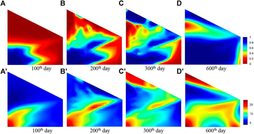
FIGURE 12. The ferrofluid saturation and magnetic anomaly distribution at different time. (A–D) respectively show the ferrofluid saturation at 100th, 200th, 300th, 600th day; (A′–D′) respectively show the magnetic anomaly at 100th, 200th, 300th, 600th day.

As shown in Figure 13, the magnetic anomaly curve of the monitoring spot S3 in the northern part of the reservoir began to rise rapidly (the dotted red line is without a strong magnetic field) after EM2 was applied. This reflects the rapid increase of ferrofluid saturation, meaning that the ferrofluid is guided to displace to the northern part of the reservoir.

FIGURE 13

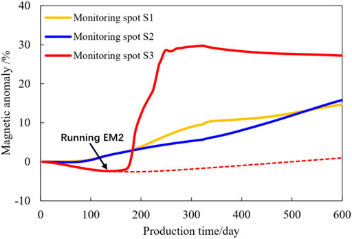
FIGURE 13. Magnetic anomaly curves of monitoring spots located in different region when apply EM2.

In addition, the water flooding is simulated for the same reservoir. Due to the large difference in oil and water viscosity, the injected water is easier to flow along the high permeability zone to the production well. Therefore, the scope of water flooding in the reservoir is smaller, and there is a large amount of remaining oil in the northern area of the reservoir that has not been displaced, as shown in Figure 14. After 600 days of production, the oil recovery of water flooding is 63.3%, and the oil recovery of ferrofluid flooding under the control of an external magnetic field is 79.5%.

FIGURE 14

FIGURE 14. The water saturation and magnetic anomaly distribution at different time. (A–D) respectively show the water saturation at 100th, 200th, 300th, 600th day.

Conclusion

In this paper, a novel ferrofluid flooding method was proposed. The ferrofluid plays the dual role of “tracer” and displacement fluid in the flooding process, that is, the flooding process can be monitored and the flooding path can be controlled.

The simulation results show that: 1) By monitoring the magnetic anomaly change information in different areas of the reservoir, the flow direction of the injected ferrofluid can be reflected, so that the heterogeneous characteristics of the reservoir can be understood; 2) The displacement direction can be changed artificially by applying a strong magnetic field to further improve the sweep range; 3) Compared with the traditional water flooding, the monitoring-controlling integrated ferrofluid flooding technology can greatly improve oil recovery.

However, there are still many problems and challenges in applying ferrofluid flooding technology. For example, how electromagnets are placed in the field and the retention loss of ferrofluid during flooding process. In the future, the authors will develop the ferrofluid flooding numerical simulation method for three-dimensional problems, and carry out ferrofluid flooding experimental research to further verify the feasibility of this technology. Nevertheless, the research in this article can still provide new ideas and theoretical guidance for further enhancing oil recovery.

Data Availability Statement

The original contributions presented in the study are included in the article/Supplementary Material, further inquiries can be directed to the corresponding author.

Author Contributions

TH conceived the idea and wrote the manuscript. FS, RW, and XH contributed to the study and gave final approval for the manuscript.

Funding

This work was supported by the Fundamental Research Funds for Zhejiang Provincial Universities and Research Institutes (Grant No. 2020J00009), the National Natural Science Foundation of China (Grant No.52004246); the Natural Science Foundation of Zhejiang Province (Grant No. LQ20E040003, Grant No.LY20D020002); the Science and Technology Project of Zhoushan Bureau (Grant No. 2021C21016).

Conflict of Interest

The authors declare that the research was conducted in the absence of any commercial or financial relationships that could be construed as a potential conflict of interest.

Publisher’s Note

All claims expressed in this article are solely those of the authors and do not necessarily represent those of their affiliated organizations, or those of the publisher, the editors and the reviewers. Any product that may be evaluated in this article, or claim that may be made by its manufacturer, is not guaranteed or endorsed by the publisher.

References

Borglin, S., Moridis, G., and Oldenburg, C. (2000). Experimental Studies of the Flow of Ferrofluid in Porous Media[J]. Transport in Porous Media 41, 61–80. doi:10.1023/a:1006676931721

CrossRef Full Text | Google Scholar

Fan, X., Sun, M., Sun, L., and Xie, H. (2020). Ferrofluid Droplets as Liquid Microrobots with Multiple Deformabilities. Adv. Funct. Mater. 30, 2000138. doi:10.1002/adfm.202000138

CrossRef Full Text | Google Scholar

Han, D. (1995). Discussion on Deep Development of High Water-Cut Oilfields Enhance Oil Recovery Problem[J]. Pet. Exploration Develop. 22 (2), 47–55.

Google Scholar

Han, D. (2010). Discussions on Concepts, Countermeasures and Technical Routes for the Redevelopment of High Water-Cut Oilfields[J]. Pet. Exploration Develop. 37 (5), 583–591. doi:10.1016/S1872-5813(11)60005-4

CrossRef Full Text | Google Scholar

Han, D. (2007). Precisely Predicting Abundant Remaining Oil and Improving the Secondary Recovery of Mature Oilfields[J]. Acta Petrolei Sinica 28 (2), 73–78. doi:10.3321/j.issn:0253-2697.2007.02.013

CrossRef Full Text | Google Scholar

Hou, H., Zhang, S., and Yang, N. (1999). Development on the Hydro-Magnetic Technology and its Application[J]. Vacuum Tech. Mater. 5, 8–12.

Google Scholar

Kamminga, W. (1975). Finite-element Solutions for Devices with Permanent Magnets. J. Phys. D: Appl. Phys. 8 (7), 841–855. doi:10.1088/0022-3727/8/7/017

CrossRef Full Text | Google Scholar

Moridis, G. J., Borglin, S. E., and Oldenburg, C. M. (1998). Theoretical and Experimental Investigations of Ferrofluids for Guiding and Detecting Liquids in the Subsurface. Office of Scientific & Technical Information Technical Reports.

Odenbach, S. (2008). Magnetoviscous Effects in Ferrofluids. Springer Berlin Heidelberg.

Oldenburg, C. M., Borglin, S. E., and Moridis, G. J. (2000). Numerical Simulation of Ferrofluid Flow for Subsurface Environmental Engineering Applications[J]. Transport in Porous Media 38, 319–344. doi:10.1023/a:1006611702281

CrossRef Full Text | Google Scholar

Oldenburg, C., and Moridis, G. (1998). Ferrofluid Flow for TOUGH2. Office of Scientific & Technical Information Technical Reports.

Rahmani, A. R., Bryant, S., and Huh, C. (2014). Crosswell Magnetic Sensing of Superparamagnetic Nanoparticles for Subsurface Applications[J]. SPE J.

Rahmani, A. R., Bryant, S. L., and Huh, C. (2015). Characterizing Reservoir Heterogeneities Using Magnetic Nanoparticles[A]. Proceedings of the SPE Reservoir Simulation Symposium[C]. Houston: Society of Petroleum Engineers.

Google Scholar

Raj, K., and Moskowitz, R. (1990). Commercial Applications of Ferrofluids[J]. J. Magnetism Magn. Mater. 85, 233–245. doi:10.1016/0304-8853(90)90058-x

CrossRef Full Text | Google Scholar

Rosensweig, R. E. (1997). Ferrohydrodynamics[M]. New York: Dover Publications Inc.

Scherer, C., and Figueiredo, A. M. (2005). Ferrofluids: Properties and Applications[J]. Braz. J. Phys. 35, 718–727. doi:10.1590/s0103-97332005000400018

CrossRef Full Text | Google Scholar

Schmidt, H. K., and Tour, J. M. (2012). Methods for Magnetic Imaging of Geological Structures [M]. Google Patents.

Sengupta, S. (2012). “An Innovative Approach to Image Fracture Dimensions by Injecting Ferrofluids[A],” in Proceedings of the Abu Dhabi International Petroleum Conference and Exhibition[C]. Abu Dhabi: Society of Petroleum Engineers.

Google Scholar

Silvester, P., and K. Chari, M. (1970). Finite Element Solution of Saturable Magnetic Field Problems. IEEE Trans. Power Apparatus Syst. PAS-89 (7), 1642–1651. doi:10.1109/tpas.1970.292812

CrossRef Full Text | Google Scholar

Yang, L. I. (2009). Study on Enhancing Oil Recovery of continental Reservoir by Water Drive Technology[J]. Acta Petrolei Sinica 30 (3), 396–399. doi:10.3321/j.issn:0253-2697.2009.03.013

CrossRef Full Text | Google Scholar

Yu, Q. (2000). Oil Field Development Three Major Rich Areas of Large Scale Unswept Remaining Oil in Water Flooded Bedded Sanstone Reservoirs[J]. Acta Petrolei Sinica 21 (2), 45–50.

Google Scholar