Microstratigraphic Analysis of Fossil Distribution in the Lower Hornerstown and Upper Navesink Formations at the Edelman Fossil Park, NJ

Maastrichtian–Danian sediments of the Navesink and Hornerstown formations at the Jean and Ric Edelman Fossil Park of Rowan University in Mantua Township, New Jersey, have long intrigued paleontologists. Within the basal Hornerstown Formation occurs the Main Fossiliferous Layer (MFL), a regionally well-known and diverse bonebed. The lithostratigraphic and chronostratigraphic position of this fossil layer have been debated for more than 50 years, fueling debate over its origin. Herein, we present the results of a microstratigraphic analysis of the fossil composition and distribution of the MFL undertaken to rectify these discrepancies. Through methodical top-down excavation, we recorded the three-dimensional position of every fossil encountered. Three-dimensional visualization and analyses of these data in ArcGIS Pro yielded an unprecedented view of this bonebed. Most reported discrepancies about the stratigraphic placement and thickness of the MFL can be explained by the presence of two distinct fossil assemblages within this interval that are occasionally combined into a single bonebed. The stratigraphically-lower assemblage, herein termed an “oyster layer”, is geometrically-tabular and exhibits low taxonomic diversity, high abundance of the oyster Pycnodonte, and moderate taxonomic richness. The stratigraphically-higher assemblage, the MFL, occurs approximately 9 cm higher in section and exhibits high values of taxonomic diversity, fossil abundance, and taxonomic richness. Sedimentological homogeneity throughout this interval suggests that these faunal contrasts arise from the two assemblages having formed via independent taphonomic pathways. Specifically, prevalence of Pycnodonte in the oyster layer implies formation by a selective mortality event, whereas the diversity of the MFL appears to reflect a more universal agent of mortality. Spatial variations in the stratigraphic distribution of fossils within the MFL in our excavation area indicate this assemblage does not form a simple, tabular layer as previously thought and may, in part, record original bathymetry. Importantly, our definition of the MFL and detailed characterization of its stratigraphic placement are essential for future studies on the taphonomic origin and chronostratigraphy of this bonebed. Universal use of this definition would allow researchers to confidently elucidate the exact lithostratigraphic positions of precise chronostratigraphic indicators within the MFL and accurately estimate the degree of time averaging of its fossils.

1 Introduction

The Navesink and Hornerstown formations represent Maastrichtian–Danian deposits from an organic-rich, siliciclastic, shallow marine shelf composed of unconsolidated glauconitic greensands (Gallagher, 1993; Obasi et al., 2011). With a shallow dip of 0.12° (Steckler et al., 1999) to 0.08° (Esmeray-Senlet et al., 2015), the Hornerstown Formation outcrops from central New Jersey to northern Delaware. Sediments comprising this formation are heavily bioturbated (Wiest et al., 2016) and consist of homogenous greensand deposits lacking any primary sedimentary structures (Obasi et al., 2011). A bonebed comprised of more than 60 invertebrate and vertebrate taxa (Gallagher, 2003), known as the Main Fossiliferous Layer (MFL), has been identified near the base of this Formation at several localities across the region (from Monmouth to Salem counties; Gallagher, 1984; Gallagher, 1993; Landman et al., 2004; Becker et al., 2009; Obasi et al., 2011). The MFL is best known from the Jean and Ric Edelman Fossil Park of Rowan University (formerly an Inversand Company Mine), in Mantua Township, New Jersey as this has been historically the largest outcrop of sediments spanning the K/Pg boundary in the region. Edelman Fossil Park has therefore been the focus of numerous studies concerning the stratigraphy and paleoecological transitions across the K/Pg boundary on the Atlantic Coastal Plain (e.g., Gallagher, 1993; Gallagher, 2002; Obasi et al., 2011; Wiest et al., 2016; Esmeray-Senlet et al., 2017). However, at this important locality, reports of the thickness of the MFL and its stratigraphic position above the underlying Navesink Formation vary greatly among many of these investigations. Additionally, the origin of this bonebed has received various interpretation, such as a reworked lag deposit (Minard et al., 1969; Kennedy and Cobban, 1996; Gallagher, 2002; Landman et al., 2012; Horner et al., 2016; Esmeray-Senlet et al., 2017), condensed assemblage (Gallagher and Parris, 1996; Olsson et al., 2002; Gallagher, 2003, Gallagher, 2012; Wiest et al., 2016), or thanatocoenosis (Gallagher, 1993; Obasi et al., 2011).

Previous studies of the MFL conducted at Edelman Fossil Park vary in their reports of the thickness and taxonomic composition of the MFL, and its stratigraphic relationship to the Hornerstown-Navesink formational boundary (summarized in Table 1 and Supplementary Figure S1). Gallagher (1993) and Staron et al. (2001) each reported the MFL as 30 cm thick but in varied stratigraphic positions above the Navesink Formation. Similarly, Obasi et al. (2011) suggested the MFL was between 20 and 30 cm thick and roughly 10 cm above the Navesink. Alternatively, Wiest et al. (2016) reported the MFL as approximately 10 cm thick and 20 cm above the Navesink, and Horner et al. (2016) proposed an intermediate thickness of 10–20 cm while agreeing with Wiest et al. (2016) on its position above the Navesink. Most recently, Esmeray-Senlet et al. (2017) reported a thickness for the MFL of 40 cm with it occurring 50 cm above the Navesink. However, in their Figure 6, Esmeray-Senlet et al. (2017) showed the MFL as approximately 30 cm thick and positioned roughly 25 cm above the Navesink, which is more comparable with previous studies. At other localities, the MFL has been reported as occurring 20 cm above the base of the Hornerstown Formation at Blackwood, NJ (Gallagher, 1984), 15 cm above the base of the Hornerstown Formation and 30 cm thick at Crosswicks Creek, NJ (Gallagher, 1993), and at a similar location as at Edelman Fossil Park at Walnridge Farm near Hornerstown, NJ (Obasi et al., 2011).

TABLE 1

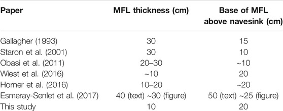
TABLE 1. Summary of reports conducted at Edelman Fossil Park characterizing the thickness of the MFL and the stratigraphic position of its base above the top of the Navesink Formation. In the row for Esmeray-Senlet et al. (2017), we list the metrics reported within the text and Figure 6 of their study, respectively.

Prior studies of the MFL have also varied in assignment of the position of the K/Pg boundary, with various workers reporting it to occur at the Navesink-Hornerstown contact (NHC; Minard et al., 1969; Owens et al., 1970; Minard et al., 1976; Self-Trail and Bybell, 1995; Kennedy and Cobban, 1996), the base of the MFL (Gallagher, 1993; Obasi et al., 2011; Gallagher, 2012; Wiest et al., 2016), within the MFL (Hope, 1999; Esmeray-Senlet et al., 2017), at the top of the MFL (Koch and Olsson, 1977), or within the Hornerstown Formation above the MFL (Olsson, 1963; Parris, 1974; Petters, 1976; Olsson and Wise, 1987; Olsson, 1988; Staron et al., 2001). This lack of consensus about the position of the K/Pg boundary in relation to the MFL continues to fuel debate over the origin of this fossil assemblage.

Much of this apparent disagreement among prior reports likely arises from the use of varied excavation/sampling methods and/or fossil collection techniques, given that identification of the stratigraphic position and thickness of the MFL were often not the primary goals. Our excavation and mapping methods, explained below, are most similar to those employed by Wiest et al. (2016), who also excavated fresh exposures with hand tools and measured the vertical position of fossils to the nearest centimeter. In contrast, Obasi et al. (2011) trenched a fresh exposure across the Navesink and Hornerstown formations for roughly 3 m to collect sediment samples and Horner et al. (2016) collected sediment samples every 5–10 cm from exposed outcrop in a similar fashion for approximately 1.6 m. Similarly, Gallagher (1993) gathered a detailed stratigraphic section at Edelman Fossil Park, recording within it a stratigraphic position and thickness of the MFL. Esmeray-Senlet et al. (2017) are the only authors to assign the position and thickness of the MFL based solely on analyses of sediment samples from a core taken at the Edelman Fossil Park just east of the current quarry. In most of the other prior studies cited above, researchers either 1) coarsely examined the stratigraphy of outcrops or well cores spanning the NHC across south-central New Jersey (e.g., Minard et al., 1969; Petters, 1976) or 2) studied fossil specimens in museum collections (e.g., Kennedy and Cobban, 1996; Staron et al., 2001).

As the stratigraphic position, thickness, and taxonomic composition of the MFL are critical information for resolving the debated aspects of this bonebed, a detailed study was necessary to elucidate these attributes. Resolving the precise stratigraphic position of the MFL is crucial for accurately correlating studies which will, in turn, help clarify the formational history of this intriguing bonebed. In the end, we quantitatively evaluate 1) prior qualitative claims of stratification of fossils within the lower Hornerstown Formation (Gallagher, 1993) and 2) the paleoecology and taphonomy of fossils within this interval.

2 Methods

2.1 Field Collection

A 1 m² area within our larger, long-term excavation project (totaling over 200 m² to date) was selected for detailed examination in this study (Figure 1A). The size and map-view location of each fossil in this square meter area were recorded by hand on a 1:1 scale paper map at the field site. After removing approximately 1 m of overburden, every fossil unearthed from 55 cm above and 5 cm below the Navesink-Hornerstown contact (NHC), regardless of size or completeness, was mapped (with a specimen’s stratigraphic position recorded based on its highest point for feasibility; see Supplementary Material for more details), collected, prepared, and identified to the least inclusive taxonomic unit possible. All fossils are reposited with unique identifiers in the Edelman Fossil Park Collection at Rowan University.

FIGURE 1

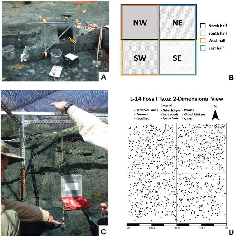
FIGURE 1. Overview of our excavation area, mapping apparatus, data partitioning system, and recovered fossils. (A) The metal frame installed around our in-progress excavation. (B) Partitioning of our excavation area by halves and quadrants. In a second stage of analyses, fossil occurrences were binned within these subregions to examine spatial variations in the geometry of fossil layers (see main text for further details). (C) Example of our three-dimensional mapping technique, in which a plum bob suspended from a scaled, movable bar across the top of the metal frame was used to measure down to the highest point of a fossil. In this case, an excavator is pointing to the fossil, a Cucullaea steinkern, whose position is being measured. (D) The digitized centroids of all collected fossils in map view, color coded by taxonomic category as shown in the legend.

2.2 Statistical Analyses

Plumb bob measurements (Figure 1C) were converted to positions above or below the NHC and graphed against specimen abundance using 1 cm intervals to track stratigraphic position. To examine fossil distribution patterns at several spatial scales, we explored trends in the data across the whole square meter as well as in spatial subsets of halves and quadrants (as portrayed in Figure 1B). Peaks in fossil abundance data for the entire square meter were delineated by counts >40; therefore, > 20 was used as a cutoff point when examining the data in spatial halves and ≥10 was used when examining the data in quadrants. Simpson Diversity Index (SDI) and taxonomic richness values were calculated using all fossil fragments because assignment of isolated and disarticulated fossils to the same individual is rarely possible at this locality (Boles, 2016) and many fossils cannot be identified to the species level due to incompleteness. For more information on how these metrics were calculated, see the Supplementary Material. For classification purposes, Xylophagella specimens were counted within the “plant remains” category (rather than the “bivalve” category) because they consist of trace fossils (boring casts) formed within driftwood without any portion of the pholadid bivalve remaining (Gabb, 1860).

2.3 Spatial Analyses

The 3D position of each fossil was further analyzed in ArcGIS Pro in order to capitalize on the ability of GIS software to quantitatively evaluate and visualize three-dimensional (3D) spatial relationships. To enable these analyses, we first converted our paper field map to a digital data record through the process of georectification within a Geographic Information System. High-resolution digital photographs were rectified to a 1:1 scale cartesian grid using ArcMap 10.6. The visual centroid of each fossil was recorded and labeled with each specimen’s unique identifier, which were then joined by attribute to the data recorded in the field and laboratory. For all ensuing spatial analyses, taxonomic units were combined into broader taxonomic categories (e.g., Gastropoda, Chondrichthyes) to permit visualization across the volume. 2D visualizations of the spatial data were created to view all fossils, each taxonomic category separately, as well as by 1 cm stratigraphic bins.

Three-dimensional visualization was conducted in ArcGIS Pro 10.8 by creating a local scene for the same spatial reference grid and using the elevations of specimens in relation to the NHC. Concave hull polygons were created for the spatial data of each broad taxonomic category using the Minimum Bounding Volume tool, enabling visual comparison of the geometric trends of each group by transparently overlaying their enclosing geometries to examine internal vertices and those externally concealed by opaque overlay. A low stratigraphic peak in abundance (later termed the “oyster layer”) was visualized as a single concave hull of all oysters in the 2D-analysis defined range of 7–19 cm above the NHC. Additionally, we used the Near 3D Tool of ArcGIS Pro to calculate the 3D Euclidean distance from each Pycnodonte and identified those within a 1 cm search radius in any direction (see Supplementary Material for more details).

Since a stratigraphically-higher peak in abundance (determined to correspond to the MFL below) contains the highest concentrations of Cucullaea vulgaris clams, plant remains (primarily Xylophagella wood borings), and tetrapod bones (see below), these taxa were used to approximate the shape of this layer in 3D. To verify that these fossils comprise a single fossil horizon, as would be expected based on prior studies (e.g., Gallagher, 1993; Gallagher, 2003; Boles, 2016), we looked at the intersection of their individual concave hulls using the Intersect 3D Tool, exploring the apparent visual overlap of their spatial extents, and potential correlation of their relative slopes. Prior to this analysis, the highest Cucullaea fossil was identified as an outlier, and it was thus not considered. We intersected the tetrapod bones and plant hulls to create a new hull consisting only of the overlapping regions. By visualizing this new hull and the Cucullaea hull simultaneously, we were then able to compare their spatial extents with the 2D spatial data, individual concave hulls, taxonomic composition metrics, and specimen abundance data to delineate the number of distinguishable fossil layers and their stratigraphic bounds.

Minimum and maximum inter-quadrant slope models were calculated for each specimen abundance peak to describe their 3D shape. Slopes were calculated between the vertical endmember specimens of each quadrant (the topmost and bottommost points), with the minimum and maximum values in each quadrant thus constraining the upper and lower bounds of each fossil layer. For the stratigraphically-lower peak in fossil abundance, these slopes were calculated over several potential intervals suggested by the 2D statistical results in order to test the sensitivity of the stratigraphic cutoffs. These stratigraphic intervals included: 8–17 cm above the NHC, inclusive (including fossils found at either 8.0 or 17.0 cm); 8–17 cm above the NHC, non-inclusive (not including fossils found at either 8.0 or 17.0 cm, but all those within that range); 7–19 cm inclusive; and 7–19 cm non-inclusive. Slopes were also calculated for the interval suggested by the nearest neighbor calculations. For the stratigraphically-higher peak in fossil abundance, the slopes bounding the Cucullaea concave hull were compared with those of the tetrapod bones + plant intersection concave hull to determine whether these areas exhibit comparable slopes and thus could be considered to belong to the same fossil layer.

Finally, structural dip angles were calculated for upper and lower bounds based on the highest or lowest endmember points, respectively, of each stratigraphic peak in fossil abundance. Two methods were used to assign the oyster layer boundaries (fossil abundance and Nearest neighbor) and each of these intervals were used to calculate separate slope and dip values because the Nearest neighbor analysis provides an interval independent of any user biases for the region most densely filled with oysters.

3 Results

3.1 2D Statistical Analyses

Our excavation of a 1 m² by 60 cm volume yielded 1,306 specimens; 1,278 of these specimens are macrofossils, of which 15% are vertebrate remains. Fossil specimens range in size from ∼1 cm fish bones to a ∼11 cm Euclastes turtle costal, with most specimens ranging in thickness from 3 to 30 mm. These fossils were identified into 17 genus or species level taxonomic units (including four ichnospecies, with the oyster Pycnodonte dissimilaris being the most common), an additional seven broader taxonomic categories, as well as coprolites and unidentified burrow casts (Supplementary Data File S1). Among these fossils are many taxa known to be common in the MFL at Edelman Fossil Park (e.g., Pycnodonte, Cucullaea vulgaris, Odontaspis cuspidata; Gallagher, 1993; Gallagher, 2003) as well as less common taxa (e.g., Sphenodiscus lobatus, associated Euclastes wielandi remains, a partial hexanchid shark tooth), indicating that the fauna we recovered is reasonably representative of the fauna of the MFL as a whole.

When the distribution of fossil specimens is vertically collapsed into a single 2D plane (i.e., map view; Figure 1D), they appear to form a virtually uniform distribution across the entire square meter area. Only one instance of definitive fossil clustering was identified: a portion of an associated sea turtle was excavated entirely from the southwest quadrant, adjacent to where additional remains of this turtle were recovered during our ongoing excavation in the months preceding this project. Associated and partially articulated skeletons are known to be fairly common in the MFL (Gallagher, 1993; Boles, 2016; Ullmann and Carr, 2021), so this result is not unexpected. Additionally, the only regions exhibiting reduced fossil density or areas void of fossils occur primarily around the edges of our study area, almost certainly due to minor, inevitable erosion of these exposed unconsolidated sediments that occurred over the length of our excavation. Similarly, the boundary between the northeast and southeast quadrants also exhibits this pattern, as this region was unfortunately exposed as a wall over a winter and some minor spalling of the exposed greensand occurred despite our covering the area.

Figure 2 displays the stratigraphic distribution of fossil abundance in 1 cm bins above and below the NHC, which clearly displays a bimodal distribution within the lower Hornerstown Formation. Two peaks are present, in which fossil counts per centimeter exceed 40 for essentially continuous stratigraphic intervals (i.e., no more than a 1 cm gap wherein the specimen count drops below 40), suggesting the presence of two separate fossil layers. The stratigraphically-lower peak in abundance occurs roughly from 12 to 19 cm above the NHC and the upper peak occurs approximately from 23 to 32 cm above the NHC. However, the diversity of fossils is not consistent throughout these stratigraphic intervals: each peak in fossil abundance is composed of a distinct distribution of taxa (Figures 2, 3; Table 2).

FIGURE 2

FIGURE 2. Stacked bar graph of fossil abundances per 1 cm stratigraphic bin, color-coded by taxonomic category as shown in the legend. Dashed gray line is positioned at the contact between the Navesink and Hornerstown formations.

FIGURE 3

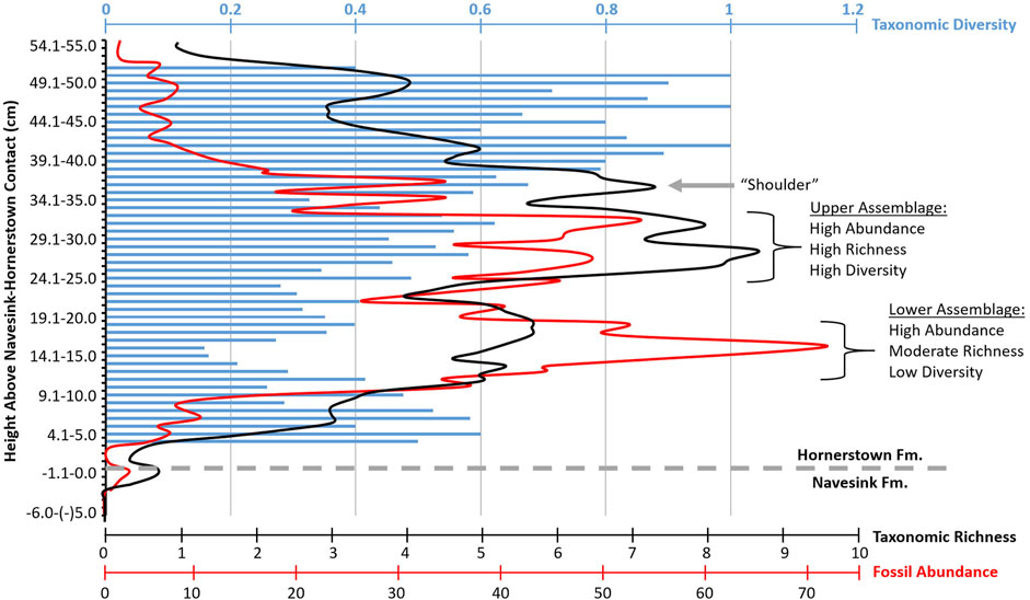
FIGURE 3. Summary of fossil abundances, Simpson Diversity Indices, and taxonomic richness per 1 cm bins in our excavation area. Taxonomic diversity values (= Simpson Diversity Indices) are shown as blue bars. Taxonomic richness and fossil abundance counts are each summarized by three-point running average curves, shown as the black and red lines, respectively. The stratigraphic interval encompassed by each fossil assemblage and the “shoulder” of the MFL (described in the text) are labeled, along with compositional characteristics of each fossil assemblage.

TABLE 2

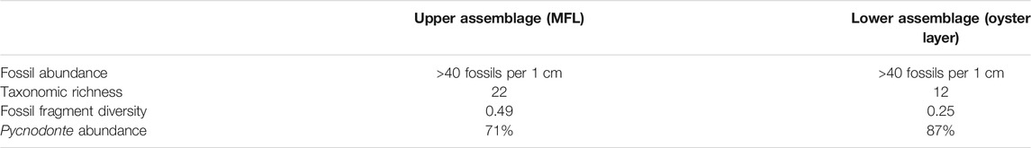
TABLE 2. Summary of fossil abundance, taxonomic richness, fossil fragment diversity (calculated as Simpson Diversity Indices), and percent of faunal composition represented by Pycnodonte oysters for each fossil assemblage identified herein. These values are derived from combining data across the entire thickness of each layer, with their stratigraphic bounds delineated as described in the text.

Taxonomic groups such as plants (primarily Xylophagella wood borings) and tetrapod remains were found primarily near the top of the stratigraphically-higher peak in fossil abundance. Other, more common fossils, such as Cucullaea, tended to be found more evenly throughout this upper layer. Osteichthyan and chondrichthyan remains were found more or less evenly distributed throughout all 60 cm of our excavation. Although the oyster Pycnodonte was found throughout the entire volume of sediment excavated, its dominance in the lower abundance peak is readily noticeable during excavation and analysis (Figures 2, 4). These trends are in general agreement with anecdotal evidence from our larger excavation of over 200 m² across the same stratigraphic interval at this site.

FIGURE 4

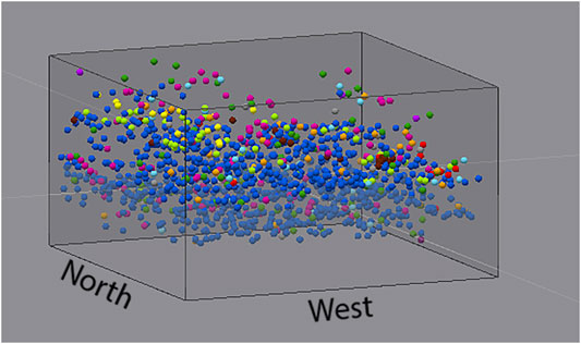
FIGURE 4. 3D map of all fossil occurrences within our study area, color-coded by taxonomic category as shown in the legend for Figure 1D.

Taxonomic richness values range from 0 to 10 in our study area across each 1 cm stratigraphic bin (Figure 3). Consistently-higher taxonomic richness values are present in the upper portion of the examined stratigraphic interval compared to in its lower portion. When stringent criteria are used to define peak intervals, then two primary richness peaks are recovered that correspond to the stratigraphic intervals of the lower and upper peaks in fossil abundance discussed above (see Supplementary Section S1.3 for further discussion of peak identification criteria). A subtle third peak in richness occurs near the top of the stratigraphically-higher richness peak, rebounding from a brief decline, wherein each 1 cm stratigraphic bin exhibits a richness ≥6. A three point running average of richness smooths some of the stochastic effects of varied fossil counts in each bin (Figure 3) and visually clarifies the extent of this subtle third peak in richness within the much more obvious, broad second peak.

Though the SDI becomes highly biased at low sample sizes, such biases are only seen in the stratigraphically highest and lowest ∼10–15 cm, outside of the intervals exhibiting peaks in fossil abundance (Figure 3). Of note, the stratigraphic interval exhibiting the lowest diversity values (<0.3) occurs from 12 to 17 cm above the NHC. This interval wholly overlaps with the stratigraphically-lower peak in fossil abundance found above. Conversely, when stratigraphic bins biased by “low” sample size (i.e., <15) are excluded, the interval exhibiting the highest diversity values (>0.5) occurs from 26 to 33 cm above the NHC. This interval wholly overlaps with the stratigraphically-higher peak in fossil abundance found above. Although these stratigraphic correlations are intriguingly consistent, it must be noted that stratigraphic bins exhibiting high fossil counts and high richness do not always also exhibit high diversity values (e.g., the bin from 18 to 19 cm above the NHC).

Percent composition of Pycnodonte, which was calculated as an additional means of tracking faunal diversity by 1 cm stratigraphic bins (see Methods), gradually increases down section (Supplementary Data File S1). Within the stratigraphically-higher peak in fossil abundance found above, the percentage of Pycnodonte varies from 28 to 62% of the fossils recovered. The stratigraphic interval exhibiting the consistently-highest percentage of Pycnodonte (>80%) occurs from 12 to 17 cm above the NHC; this interval overlaps with the stratigraphically-lower peak in fossil abundance found above.

As expected, the exact stratigraphic ranges of peaks in fossil abundance vary slightly among the examined spatial subsets compared to the whole square meter (Supplementary Data File S1). Two peaks were recovered in the south half, and they coincide in position with the two peaks identified within the full dataset (Figure 2). Though two peaks were also recovered in the north half, they occur slightly stratigraphically higher, and data from the east half exhibit three peaks. Data from the west half form a trend suggestive of the presence of two peaks, but the apparent lull between them does not satisfy the criterion to split the trend into two separate peaks (see Supplementary Section S1.1 for further discussion of peak stratigraphic intervals). To more finely characterize these spatial variations in the stratigraphic bounds of the two apparent fossil layers, we further parsed the specimen occurrence data into quadrants (Supplementary Data File S1). The stratigraphic intervals of peak fossil abundance recovered in each quadrant are detailed in section 1.1 of the Supplementary Material. As when the abundance dataset was partitioned into halves, quadrants also show variation in the number and stratigraphic position of peaks, with one to four peaks being identified among quadrants. Cumulatively, these results from spatial subsets reveal that the northern portion of our excavation exhibits both broader stratigraphic dispersion of fossils and slightly stratigraphically-higher peaks in fossil abundance than found across the entire square meter as a whole.

3.2 3D Analyses

Here, we first consider concave hulls created from the positional data of specimens belonging to our broad taxonomic categories. Each concave hull calculated for a taxonomic category exhibits a unique 3D geometry (Supplementary Figure S2). Pycnodonte specimens form a relatively amorphous shape with two higher peaks in the northwest and southeast quadrants (Supplementary Figure S2A). Compared to Pycnodonte, chondrichthyan specimens form a visually “opposite” amorphous shape with lower protrusions in the northwest and southeast quadrants (Supplementary Figure S2B). The geometry of the tetrapod bone concave hull, in contrast, is relatively flat at the top of its stratigraphic bounds, with the highest specimens in the northwest and lowest specimens in the southwest quadrant (Supplementary Figure S2C). Similarly, plant fossils form a planar hull that is tilted stratigraphically upward to the northwest (Supplementary Figure S2D). The concave hull calculated for Cucullaea, both with and without the single high outlier removed, are also similar to those of tetrapod bones and plant fossil hulls in that they are overall flat on the bottom and curve along their tops with a northwest-trending positive slope (Supplementary Figure S2E). Burrows (Supplementary Figure S2F) and osteichthyan bones (Supplementary Figure S2G) form concave hulls that are irregularly dome-shaped, each with a gently-sloping base. Additionally, the osteichthyan bones hull exhibits a corrugated shape that gradually slopes upward toward the north. The gastropod (Supplementary Figure S2H) and other fossil specimens (Supplementary Figure S2I) hulls exhibit similar characteristics in that both are generally convex polygons with the lowest specimens present in the northeast.

Across the entire dataset, the average number of oysters whose nearest-neighboring oysters is within 1 cm is two, with a standard deviation of 2.3. The most dense horizon of oysters in 3D space, as identified from the stratigraphic interval exhibiting the highest frequency of oyster nearest neighbors, occurs at 16.0 cm above the NHC, with 18 oysters being within 1 cm of the nearest neighboring oyster (Figure 5); in other words, this identified the greatest abundance of closely-packed oysters occurs at that stratigraphic height. The next-highest frequency (12 oysters as nearest neighbors) occurs immediately below this maximum. From 10.6 to 19.1 cm above the NHC, frequency values consistently exceed seven, greater than two standard deviations above the mean; this is the only examined stratigraphic interval to consistently exhibit such high frequencies of neighbors. Stratigraphically beneath this region, Pycnodonte neighbor counts almost never exceed the mean, and immediately above this region occurs a 4 cm thick interval of oysters whose number of neighbors rarely exceeds one standard deviation above the mean. Above this 4 cm interval, the frequency of nearest neighbors occasionally spikes just over two standard deviations above the mean but never remains at these levels for successive heights. Thus, the stratigraphic interval from 10.6 to 19.1 cm above the NHC is statistically significant regarding its oyster density, even among other intervals within the study area which include abundant Pycnodonte fossils.

FIGURE 5

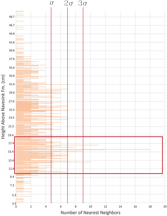
FIGURE 5. A histogram of the general abundance of the oyster Pycnodonte dissimilaris by 1 mm stratigraphic bins, presented as the number of oysters in each bin which were found to be the nearest neighbor for another oyster. Only one interval, from 10.6 to 19.1 cm above the NHC, exhibits frequency values consistently greater than two standard deviations above the mean.

The stratigraphically-lower peak in fossil abundance, as defined by our 2D analyses, displays a relatively flat geometry. Minimum and maximum inter-quadrant slope models of this layer (Table 3) show the most consistent geometry from the 2D model occurs from 7 to 19 cm above the NHC. Slope values for the top and base of this layer are all very close to zero (Table 3). Dip angles calculated based on the concave hull and the nearest-neighbor-defined lower fossil layer (see Methods) were also found to be zero or near zero (Table 4), in general agreement with these low slope values.

TABLE 3

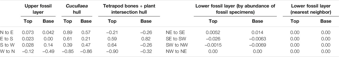
TABLE 3. Comparison of calculated slope values for the top and base of both fossil layers identified herein within the lower Hornerstown Formation. The Cucullaea hull slopes are values from the specimens one standard deviation below and two above the mean height. The upper fossil layer slopes pertain to a combination of the Cucullaea hull specimens with those forming the tetrapod bones + plant intersection hull. The last set of slopes was calculated from the most concentrated region of specimens found by the nearest neighbor analysis. All directions are abbreviated.

TABLE 4

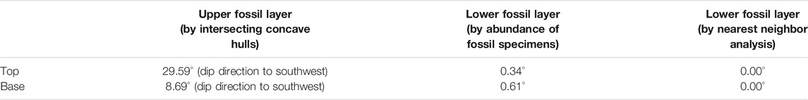
TABLE 4. Maximum dip angles of the top and base planes of both fossil layers identified herein relative to the Navesink-Hornerstown formational contact. For comparison, the structural dip of the Hornerstown Formation has been previously reported as ranging from 0.08° to 0.12° (Steckler et al., 1999; Esmeray-Senlet et al., 2015).

The upper fossil layer was found to be more difficult to define in 3D space due to its greater diversity; therefore, we calculated the slope of this layer using multiple definitions (Table 3). First, the stratigraphic interval encompassed by this layer was estimated by analyzing the distribution of all tetrapod bones, plant remains, and Cucullaea specimens in the entire square meter. The lower boundary of this interval was placed one standard deviation below the mean height of all specimens of these taxa (31.3 cm above the NHC). Its upper boundary was placed at two standard deviations above the mean rather than one to account for the apparent upward skew of fossil occurrences of taxa commonly or exclusively found in this higher peak in abundance. Using these bounds, our 3D analyses found the stratigraphically-higher abundance peak to occur from 23.9 to 41.4 cm above the NHC. As two alternative definitions, we also considered: 1) the geometry of the Cucullaea hull alone (Supplementary Figure S2E) as a general representation of this layer, and; 2) the sum of the volumes encompassed by the Cucullaea hull and the tetrapod bones + plant intersection hull. On visual inspection, all of these hulls exhibit similar slopes that extend downward from the northwest to southeast along the top with an overall flat bottom, as evidenced by the higher maximum dip angles on the top compared to its base (Table 4; see Supplementary Section S1.4 for more details).

Together, these findings suggest that the shape of the upper fossil layer (assigned to be the MFL, see Discussion) is not a purely tabular layer, but rather it exhibits subtle variations in “topography” which include a slightly upward slope toward the northwest within our study area. In contrast, the lower fossil layer lacks such slope variations within our study area.

4 Discussion

4.1 Recognition and Definition of Fossil Layers

Data from our microstratigraphic analyses strongly suggest the presence of two distinct fossil assemblages exhibiting stratigraphic and taxonomic heterogeneity and, presumably, differing formational histories within sediments comprising the basal Hornerstown Formation. Unlike prior studies, our explicit intent was to characterize the centimeter-scale 3D distribution of fossils within this stratigraphic interval, and this unique focus allowed us to distinguish these two distinct fossil assemblages. However, we are not the first to propose differentiation of fossils within the basal Hornerstown Formation. Gallagher (1993) proposed that the MFL is composed of several layers including a basal oyster bed with overlying vertebrate remains. Our findings quantitatively corroborate that qualitative assessment as we have identified additional taxonomic and spatial distinctions between what have been occasionally regarded as “lower” and “upper” portions of the MFL.

Evidence from our 2D analyses for the presence of two fossil horizons in the basal Hornerstown stems from all three aspects we considered: fossil abundances, taxonomic richness, and taxonomic diversity. The strong bimodal distribution of fossil abundances across the entire square meter, with a lower peak from 12 to 19 cm and an upper peak from 23 to 32 cm above the NHC, is indicative of the presence of two fossil layers (Figures 2, 3). Bimodal distributions were also found in the north half, south half, and southwest quadrant, and the general character of fossil abundances in many other data partitions (e.g., the east and west halves) is also bimodal (Supplementary Data File S1). Although the west half and northwest quadrant each exhibit just a single peak in abundance, those broad peaks appear to meld the upper and lower peaks (i.e., the assemblages) observed in other data partitions.Where a bimodal distribution is apparent, the base of the lower peak in fossil abundance consistently occurs within a 3 cm stratigraphic range (10–13 cm above the NHC) whereas its top may vary in stratigraphic position by up to 6 cm (18–24 cm above the NHC). This consistency indicates that the lower assemblage is generally structured as a tabular bed of nearly uniform thickness in stratigraphic conformity with the structural plane of the NHC. This conclusion is further corroborated by our 3D analyses of fossil distributions. Slope and dip values each remain essentially constant near zero across the top and base of this assemblage, regardless of the quantitative data examined (Table 3). Our nearest neighbor analysis identified the stratigraphic interval from 10.6 to 19.1 cm above the NHC to also form a tabular region encompassing the highest density of oysters within our excavation (Figure 5). That interval overlaps stratigraphically with the lower peak in fossil abundance (Figures 2, 3), further supporting characterization of this interval as a distinct fossil layer. Cumulatively, these findings demonstrate that this lower layer is generally tabular in form and that it dips (relative to the NHC) by less than 1°.

Since this stratigraphically-lower fossil assemblage is predominately comprised of oysters and exhibits a correspondingly-low Simpson Diversity Index, we elect to describe it as an “oyster layer” near the base of the Hornerstown Formation. Allowing for single-centimeter intervals of stochastic variation in fossil composition, this oyster layer exhibits a Simpson Diversity Index <0.3 due to >80% of its fossil specimens pertaining to the oyster Pycnodonte. Gallagher (1991) reported a similar high percentage of 78% for representation of Pycnodonte oysters within the basal Hornerstown, with this slightly lower percentage likely owing to pooling of data from the oyster layer (as defined above) and overlying MFL. The striking consistency of percent Pycnodonte and SDI throughout the oyster layer make them the best, most-reliable parameters for determining the upper and lower boundaries of the oyster layer, which in turn constrain its overall thickness within our study area. Based on these metrics, the oyster layer is 9 cm thick and extends from 8 to 17 cm above the NHC. In terms of faunal composition, the most consistent interval within the oyster layer (i.e., the portion most likely to be recognized while in the field) occurs from 12 to 17 cm above the NHC, thus pertaining to the upper portion of the assemblage. This span continuously meets the above SDI and percent Pycnodonte criteria (i.e., without single-centimeter “violations”) and contains over 40 fossils per 1 cm stratigraphic bin within the excavation area. Fossil abundances, taxonomic richness, and proportional abundance of Pycnodonte all decrease gradually down-section toward the base of the oyster layer (i.e., from 12 cm down to 8 cm above the NHC; Figures 2, 3, Supplementary Data File S1).

Multiple taphonomic scenarios could account for the gradational base of the oyster layer. Because the genus Pycnodonte is an epifaunal recliner adapted to living on soft substrates (Dhondt, 1984; Macellari, 1988; Callapez et al., 2015), the oyster layer appears to represent an autochthonous assemblage. Therefore, the gradational base of this layer could reflect: 1) a rapid mass death event followed by minor disturbance of fossil distributions via intense bioturbation of these sediments by thalassinoid crustaceans (Wiest et al., 2016); 2) a temporally-building mortality event over the order of 36 kya (cf. Esmeray-Senlet et al., 2017, based on fitting a best-fit sediment mixing model to the iridium profile), ∼75 kya (cf. Gallagher, 1993, based on dinoflagellate biostratigraphy), or ∼90 kya (cf. Obasi et al., 2011, based on glauconite maturity levels across this interval), and/or; 3) that the oyster layer assemblage formed by more random attritional accumulation. The significant taphonomic implications of each of these non-mutually-exclusive scenarios should be considered in a future study. For the moment, however, we note that the rarity of taxa other than Pycnodonte within the oyster layer indicates potentially selective die-off of oysters in an ecological event, and this character clearly contrasts what is seen in the upper fossil assemblage (the MFL, see below).

In contrast to the oyster layer, the positions of the boundaries (and therefore thickness) of the upper peak in fossil abundance are more variable. Certain spatial subpartitions, namely the south half and southwest quadrant, exhibit a position for the upper peak of fossil abundance with its base at 23 cm above the NHC and top at 28 or 32 cm above the NHC. Other subpartitions exhibit slightly greater variation, with the base and top of this upper peak in fossil abundance occurring as high as 30 and 37 cm above the NHC (in the north half), respectively. Thus, depending on how the data are partitioned, the base of this upper peak in abundance may vary in stratigraphic position by up to 7 cm and its top may vary in position by up to 9 cm.

Presumably this upper fossil assemblage should correspond to the MFL. However, prior characterizations of the MFL relied heavily on attributes beyond fossil abundance (e.g., presence of diverse vertebrate remains; Gallagher, 1993; Gallagher, 2003), so it will be helpful to briefly review the origin, evolution, and varied uses of the name Main Fossiliferous Layer over the last 50 years before assigning stratigraphic bounds to the MFL herein. The phrase “main fossiliferous layer” was originally used by Parris (1974) as an informal term for the most prolific fossil-bearing assemblage in the lower Hornerstown Formation at Edelman Fossil Park, then an Inversand Company mining quarry. Gallagher (1984) informally synonymized Parris (1974) “main fossiliferous layer” with other informal names historically applied to this layer, such as the lower Hornerstown “bonebed” (White, 1972; Richards and Gallagher, 1974; Gaffney, 1975), while also capitalizing the name MFL for the first time; this began continued use of the term Main Fossiliferous Layer as a formal name for this prolific assemblage (e.g., Gallagher et al., 1986; Parris et al., 1986). However, to our knowledge, no study has ever used precise, quantitative methods to define the stratigraphic extent or faunal characteristics of the MFL. Therefore, below we propose unique, spatially-consistent trends within our data as defining attributes of the MFL in order to help standardize use of this name in future studies, which is direly needed given the frequent inconsistencies in application of this name in recent years (summarized in Table 1 and Supplementary Figure S1).

At least a portion of what most authors have previously called the Main Fossiliferous Layer clearly corresponds to the upper fossil assemblage identified herein. Based on the distribution of fossils in our excavation area and their taxonomic identities, we distinguish the MFL as solely pertaining to this upper assemblage. Specifically, throughout the entire interval from 23 to 33 cm above the NHC, at least one of the following criteria are met: fossil count >40 per 1 cm stratigraphic bin; SDI ≥0.5, and/or; taxonomic richness ≥7 (Figure 3). At least two of these metrics are met from 24 to 32 cm above the NHC, signifying that this interval represents the most consistent portion of the MFL and the most likely interval to be recognized while in the field. Fossil abundances and taxonomic richness each decrease rapidly below and above this 8 cm stratigraphic interval, indicating that the MFL exhibits relatively sharp basal and upper bounds. SDI values also decrease away from this interval, but at a lesser rate. Owing primarily to fossil occurrences within the north half of the excavation area, richness and SDI (but not fossil abundance) values for the entire square meter each increase again to levels characteristic of the MFL over a thin stratigraphic interval just above the MFL as defined above. This is particularly evident from 35 to 37 cm above the NHC, which corresponds to 3–5 cm above the MFL, wherein both taxonomic richness and SDI values meet the metrics used to define the MFL. We therefore term this thin interval a “shoulder” of the MFL (Figure 3).

To further explore this question, we used spatial analysis tools in ArcGIS Pro to examine patterns in the 3D occurrences of fossils with greater (0.1 cm) resolution. Our study is one of the first to use 3D GIS methods for the purpose of not only analyzing fossil assemblages in high-scale resolution, but of also defining their planimetric and stratigraphic extents (see Supplementary Section S1.5 for more on our digital methodological advancements). Several lines of evidence indicate the upward-sloping “shoulder” of the MFL is a genuine feature of this layer’s geometry within our excavation area rather than an artifact of our data processing methods. First, the concave hulls of several key groups which may be considered representative of the fauna of the MFL, such as tetrapod bones, plant remains (wood and Xylophagella boring casts), and Cucullaea clams, each display a dramatically-positive, northerly tilt, as does their combined intersection hull, created to represent the general form of the MFL in 3D (Figure 6). Concave hulls of other, more stratigraphically-distributed taxonomic categories such as fish bones also display northern tilts, but of gentler slopes (Supplementary Figure S2). Visual examination of the entire dataset in 3D (Figure 4) also reveals an upward tilt of diverse fossils toward the north half of our excavation area, which cumulatively create the “shoulder” of the MFL seen in our 2D analyses. Additionally, our dip calculations of the MFL from our 3D analyses are consistent with the understanding that the top of the MFL is more steep than its base, which is consistent with our 2D findings but inconsistent with the near-horizontal dip of the NHC and oyster layer (Table 4).

FIGURE 6

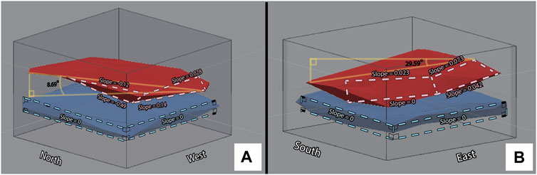
FIGURE 6. 3D representations of the MFL (red) and oyster layer (blue) shown as concave hulls in opposing oblique views. The MFL is represented by the bone + wood intersection hull overlapped with the Cucullaea fossils from two standard deviations above and one below their mean height. The oyster layer is represented by oysters from the stratigraphic interval identified as having the most neighbors within a 1 cm radius of any other given oyster in that interval. (A) Northwest view. (B) Southeast view. The top and baselines of the areas circumscribed by dashed lines were used for calculating slope values for each fossil layer, which are annotated along each corresponding margin. Right triangles shown in yellow were used to calculate maximum dip angles (written in black text) between specimens occurring along the base of the MFL (A) and top of the MFL (B).

Such variations in stratigraphic position and thickness of the MFL suggest that it does not form a simple, tabular layer but instead exhibits small-scale undulations or a tilt that do not match the structural dip of the Hornerstown Formation in southern New Jersey (0.08–0.12°, Steckler et al., 1999; Esmeray-Senlet et al., 2015). In contrast, the oyster layer displays considerably less variation in its stratigraphic position and thickness. Thus, the two layers do not form planes parallel to one another within our excavation area, and the MFL in particular appears to exhibit a slight overall tilt relative to the NHC and oyster layer that cannot be accounted for by structural dip. This implies that the sedimentary and/or taphonomic processes which created unevenness within the MFL are temporally constrained to have occurred after deposition of the oyster layer. Although sediments at this site have been heavily bioturbated by decapod crustaceans (presumably cf. Hoploparia sp.; Gallagher, 2003), it is highly unlikely that bioturbation can account for the stratigraphic separation and contrasting diversity metrics of these fossil assemblages because: 1) crustaceans are documented to have been burrowing throughout this entire timespan (not just during deposition of the MFL; Wiest et al., 2016), and; 2) the vast majority of macrofossils collected in this study (e.g., Cucullaea steinkerns, Pycnodonte valves) are much larger than the average diameter of the Thalassinoides burrows within this interval (∼1.1 cm; Wiest et al., 2016). Therefore, other explanations must be examined. Indeed, few options remain that could explain these small (<10 cm of stratigraphic variation over 1 m of distance) but noticeable (during excavation) variations in stratigraphic geometry of the MFL.

One potential explanation for the complex geometry of the MFL is that we have identified natural variations in paleobathymetry over which the fossil organisms lived and died. Centimeter to multiple decimeter-scale variations in seafloor topography within a single square meter area are common on the shallow shelf owing to currents and the actions of bioturbators (e.g., Wang and Tang, 2009; Schönke et al., 2017), both of which would have also exerted influences on the seafloor topography at Edelman Fossil Park at the time of deposition of the MFL. Therefore, we hypothesize that the subtly-undulatory geometry of the MFL may have arisen from these processes, with bioturbation likely playing a major role (e.g., Hoploparia and/or other small crustaceans likely made spatially-heterogeneous mounds of sediments on the seafloor as they excavated Thalassinoides burrows; cf. Felder, 2001; Rodríguez-Tovar et al., 2010). Although this hypothesis requires confirmation from additional 3D mapping of fossil occurrences over a larger area, it could plausibly explain the comparatively even/uniform character of the southern half of the MFL and its gradual slope upward toward the north. An alternative hypothesis of a local east-west trending fault is not supported by our data because the MFL fossil data points form a gradual slope rather than a stepped offset (Figures 4, 6). Additionally, any such fault would have to have been an extremely small-scale feature (i.e., a “microfault”) as fossils within the underlying oyster layer do not exhibit a similar slope/step, nor does the NHC. Still, other alternative hypotheses remain plausible, such as attritional accumulation of organic remains over a short period of time (<250 kyr; Gallagher, 1993), resulting in them being preserved at multiple stratigraphic horizons within the MFL. The continuous, gentle nature of the slope in MFL fossil positions (Figures 4, 6), however, seems difficult to account for by attritional accumulation alone, which (by definition) would usually be expected to yield more erratically-positioned fossils. Repetition of this study over a larger geographic area would be required to fully evaluate any of these taphonomic hypotheses.

To examine the faunal profile of each fossil assemblage, we combined fossil occurrence data from the stratigraphic bins encompassed by each layer and then calculated an average taxonomic richness, Simpson Diversity Index, and percent Pycnodonte for each pooled dataset. This reanalysis found the 9 cm interval encompassing the oyster layer (8–17 cm above the NHC) to be composed of 87% Pycnodonte with an SDI of 0.25 and taxonomic richness of 12. In contrast, the 10 cm interval encompassing the MFL (23–33 cm above the NHC) contains a lower percentage of Pycnodonte (71%) and substantially higher SDI (0.49) and taxonomic richness (22) values. Thus, contrasts in taxonomic richness, diversity, and proportional abundance of the oyster Pycnodonte further enhance distinction between these two assemblages initially identified by peaks in our fossil abundance data.

Finally, although our thorough analyses have elucidated many contrasting features about these two fossil layers that will aid ongoing efforts to understand the formative history of the MFL and faunal changes occurring across the K/Pg boundary in the northern Atlantic Coastal Plain, several of these distinguishing characteristics of each layer would be difficult to identify in the field. We therefore propose the following “field definitions” of the oyster layer and MFL to facilitate their recognition in the field. The oyster layer begins roughly 10 cm above the NHC, is approximately 5–10 cm thick, and is marked by a great abundance of fossils, primarily Pycnodonte oysters with occasional specimens of other taxa. The MFL, by contrast, begins a little over 20 cm above the NHC contact, is roughly 10 cm thick on average, contains more fossils than the oyster layer (N = 420 versus 366, respectively; Supplementary Data File S1), and fossils within it pertain to a considerably more diverse suite of taxa, including plants (primarily Xylophagella wood boring casts) and large vertebrates (e.g., turtles, crocodilians, and mosasaurs). Specimens of Cucullaea vulgaris are likely to be encountered frequently within the MFL (Gallagher, 1991), but this taxon is not especially numerous nor uniformly distributed spatially; therefore, wood and tetrapod remains (i.e., bones and teeth) are also useful fossils for identifying the MFL while in the field. Further, Cucullaea vulgaris specimens can also be found both above and below the MFL, so recovery of a single individual of this bivalve is not enough to identify the position of the MFL. It is true, however, that within strata near the NHC, steinkerns occur most commonly in the MFL [Figure 2, and Gallagher (1993)]. The gap between the base of the MFL and the top of the oyster layer can vary from approximately 5–10 cm, which can be recognized during top-down excavation by a relative drop in the number and diversity of fossils recovered. These field definitions, based on the 1 m² area studied herein, are additionally supported by anecdotal observations from our larger systematic excavation of over 200 m² through the same stratigraphic interval at Edelman Fossil Park.

4.2 Comparisons With Previous Studies

Comparing the stratigraphic extent of the MFL as defined herein to its position and thickness as described in previous reports (Table 1, Supplementary Figure S1) reveals that much of the variation among studies can likely be attributed to the use of varied stratigraphic thickness and position for this layer and the diverse methodologies that researchers have used to study it. For instance, studies which have reported the MFL to be 20 cm or more thick (Gallagher, 1993; Staron et al., 2001; Obasi et al., 2011) have clearly included the oyster layer within their assignment of the MFL. This is not surprising given how the two assemblages occur in very close stratigraphic proximity and together form an obvious, broad peak in fossil abundance compared to the strata overlying and underlying them which contain considerably fewer fossils (as also evidenced by our data; Figures 2, 3). However, our findings strongly support stratigraphic, paleoecologic, and taphonomic distinction between these two fossil assemblages. Consideration of the oyster layer as a basal portion of the MFL would also explain most differences in the reported placement of the base of the MFL by prior studies, as this would result in a lower base for the “assemblage” as a whole (as interpreted by Gallagher, 1993; Staron et al., 2001; Obasi et al., 2011). For example, the 30 cm thickness reported by Staron et al. (2001) suggests that they included the oyster layer within the MFL, and their report of the base of the MFL as being 10 cm above the NHC further supports this conclusion as that is roughly the location of the base of the oyster layer as defined herein. Therefore, we suggest that, stratigraphically, the majority of prior reports actually agree more than the reported values suggest, and the differences reported in Table 1 simply stem from varied assignment of the MFL.

Based on our data, we agree with Wiest et al. (2016) and Horner et al. (2016) that the MFL is quite thin and that small magnitude variations in thickness of the MFL exist (e.g., 10–20 cm; Horner et al., 2016). We add that this variation is likely due to the weakly-undulatory, non-tabular geometry of this layer identified herein. Additionally, this new, formal definition restricts the name Main Fossiliferous Layer to pertain specifically to the highly-diverse fossil assemblage in the lower Hornerstown Formation which most researchers have been interested in studying due to its potential connections with the K/Pg mass extinction. The only prior report whose claims we cannot reasonably reconcile with these conclusions is that by Esmeray-Senlet et al. (2017), who reported uniquely higher numbers for the base and thickness of the MFL (Table 1). We speculate that the uniqueness of their results might have arisen from uncertainties involved in assigning the placement of the MFL within the limited sample volume of a drill core.

Defining the stratigraphic boundaries and thickness of the MFL is important for characterizing both its formational history and chronostratigraphic relation to the K/Pg boundary. For example, assuming a relatively constant sedimentation rate [based on glauconite maturity (Obasi et al., 2011) and dinoflagellate biostratigraphy (Koch and Olsson, 1977)], the 10 cm thickness definition proposed herein suggests that the MFL was deposited over a shorter timeframe than inferred from many prior, thicker estimates (e.g., Gallagher, 1993; Staron et al., 2001; Obasi et al., 2011; Esmeray-Senlet et al., 2017), which in turn suggests that [in agreement with Boles (2016) and Wiest et al. (2016)] fossil remains in the MFL are less time averaged than some have thought. Additionally, when the definition of the MFL proposed herein is applied to prior reports (listed in Table 1) of the location of the K/Pg boundary, the chronostratigraphic location of this boundary changes from the base of the MFL in Gallagher (1993) and Obasi et al. (2011) to actually occur at the base of the oyster layer (Obasi et al., 2011) and in the middle of the oyster layer (Gallagher, 1993). Therefore, they no longer agree with the placement of the K/Pg boundary by Wiest et al. (2016) and Horner et al. (2016) which remain at the base of the MFL. Furthermore, using this definition of the MFL, Esmeray-Senlet et al. (2017) actually placed the K/Pg boundary well above the top of the MFL, in general agreement with Staron et al. (2001). Prior reports that placed the K/Pg boundary at the NHC (e.g., Minard et al., 1969; Self-Trail and Bybell, 1995) are not affected by any definition of the MFL. It is not possible to reconcile any other prior claims about the position of the K/Pg boundary (e.g.; by Olsson, 1963; Petters, 1976) into the precise centimeter-scale stratigraphic framework examined herein as they did not report a precise stratigraphic position nor thickness of the MFL. Nevertheless, the discrepancies among the studies reconciled above emphasize the need for all future researchers to employ the same definition of the MFL. Universal use of the same definition will allow any precise geochronologic indicators (e.g., shocked quartz, spherules) or other signals of environmental disturbance found in this interval in the future to be placed in their exact chronostratigraphic positions relative to this fossil assemblage. Only then can the origin of the MFL and any connection it may have with the Chicxulub impact (Obasi et al., 2011) truly be discerned with certainty.

Since herein we did not search for nor collect any precise geochronologic indicators, we can only attempt to synthesize prior claims about the position of the K/Pg boundary. Prior researchers have used a wide variety of methods to discern the position of this boundary (i.e., geochemistry, ichnology, biostratigraphy), and few studies have employed the same techniques. For example, among the studies reconciled in the previous paragraph, only Esmeray-Senlet et al. (2017) made their assignment based directly on a precise indicator of the Chicxulub impact event (an iridium spike). Wiest et al. (2016) alternatively placed the K/Pg boundary based on an abrupt reduction in the average diameter of Thalassinoides burrows, which Horner et al. (2016) found to be accompanied by a shift in the elemental composition of the sediments infilling burrows. One possible hypothesis to reconcile these data and the associated contrasts in placement of the K/Pg boundary among studies could be the following: given that 1) iridium-rich dust was likely settling through the water column to the seafloor for a period of several years [Vellekoop et al. (2016), and references therein] after the moment of impact [which defines the geochronologic K/Pg boundary; Molina et al. (2006)] and 2) iridium can be remobilized in unconsolidated sediments [e.g., Hull et al. (2011), Racki et al. (2011), Wallace et al. (1990)] whereas burrows cannot, it is plausible that iridium-rich dust predominately fell after decapod crustaceans were already constrained to smaller body sizes by post-impact environmental disturbances. This scenario would be consistent with a hypothesis that the K/Pg boundary occurs at the base of the MFL, in agreement with the conclusions of Wiest et al. (2016), Horner et al. (2016).

5 Conclusion

As the largest historically-available outcrop of sediments spanning the Navesink-Hornerstown contact, Jean and Ric Edelman Fossil Park has been an important place for research on the geology, taphonomy, and taxonomy of these regional deposits. Specifically, the Main Fossiliferous Layer within the basal portion of the Hornerstown Formation has received significant attention and has even been proposed to possibly represent a K/Pg thanatocoenosis created by environmental disturbances created by the Chicxulub impact. Various field techniques have been utilized over the years to study the MFL at this locality, which has led to variable reports of the stratigraphic placement and extent of this important bonebed. Herein, we have shown through detailed 2D and 3D spatial and statistical analyses that two distinct fossil assemblages are present in the basal Hornerstown Formation: the MFL and an “oyster layer” 5–10 cm beneath it. This is significant because inconsistent inclusion of one or both of these fossil assemblages in assignments of the MFL explains most of the differences among prior reports.

We elect to call the stratigraphically-lower fossil assemblage an oyster layer due to its tabular geometry, low taxonomic diversity, and proportional abundance of Pycnodonte oysters. This layer begins approximately 10 cm above the NHC, is approximately 5–10 cm thick, and can be recognized in the field primarily by its abundance of Pycnodonte oysters in comparison to the immediately surrounding sediments. The stratigraphically-higher fossil assemblage we identified is equivalent to previous descriptions of the MFL due primarily to its great abundance of taxonomically diverse fossils. The base of this layer occurs roughly 20 cm above the NHC and it is approximately 10 cm thick, but this assemblage may locally swell up to 10 cm higher in section while remaining only 10 cm thick. The MFL assemblage can be recognized in the field by its wealth of invertebrate steinkerns (e.g., of the bivalve Cucullaea), an overall abundance of diverse fossils, and the presence of large tetrapod (e.g., turtle, crocodile, and mosasaur bones) and plant remains (e.g., fossil wood, Xylophagella boring casts). This layer does not exhibit a simple, tabular geometry, but rather subtly slopes upward towards the north within our excavation area. Neither the NHC nor the oyster layer exhibit this slope, indicating that the process (es) which created this slope were temporally constrained to the timeframe of deposition of the MFL. This implies separate paleoecologic and taphonomic origins for the oyster layer and MFL, which clearly support their distinction as separate fossil units. We hypothesize that the complex stratigraphic geometry of the MFL possibly records subtle undulations in seafloor topography (i.e., paleobathymetry). This hypothesis could be further evaluated by performing a similar study over a wider area at this locality.

Use of ArcGIS Pro and its 3D mapping tools was essential to elucidate the distributions of taxa within and spatial geometry of each fossil assemblage. These powerful tools offer paleontologists quantitative metrics and valuable visuals for characterizing and describing bonebeds. We have demonstrated that this can be accomplished without the use of expensive field equipment if enough time is allotted for thorough data collection.

Ultimately, our quantitative confirmation of stratification of fossils within the lower Hornerstown Formation into two distinct fossil horizons allows us to reconcile the use of different definitions of the MFL in past studies. Synthesizing prior reports into a unified stratigraphic framework clarifies the current state of debate over the origin of the MFL. Specifically, the thin geometry of the MFL indicates its fossils have experienced less time averaging than would be implied by many previous reports, which adds potential support to the MFL representing a thanatocoenosis. However, future studies investigating the taphonomic origin and/or chronostratigraphic placement of the K/Pg boundary in relation to the MFL need to acknowledge previous discrepancies in the literature regarding the composition and stratigraphic placement of the MFL, as reconciled herein. Only then can any precise geochronologic indicators (e.g., shocked quartz, iridium spike) found within this interval be accurately used to interpret the taphonomic origins of these intriguing fossil assemblages.

Data Availability Statement

The original contributions presented in the study are included in the article/Supplementary Material, further inquiries can be directed to the corresponding author.

Author Contributions

PU and KL designed the study. KV, PU, MH, BK, IP, and ZB collected the field data and prepared, cataloged, and identified all fossil specimens. KV and PU analyzed the 2D data. ZC, TL, SW, and KV digitized and analyzed the 3D data in ArcGIS Pro 10.8. The first draft of the manuscript was prepared by KV, which then received input from all coauthors.

Funding

This research was supported by the Dean’s Office of the Rowan University School of Earth and Environment and the Jean and Ric Edelman Fossil Park of Rowan University.

Conflict of Interest

The authors declare that the research was conducted in the absence of any commercial or financial relationships that could be construed as a potential conflict of interest.

Publisher’s Note

All claims expressed in this article are solely those of the authors and do not necessarily represent those of their affiliated organizations, or those of the publisher, the editors and the reviewers. Any product that may be evaluated in this article, or claim that may be made by its manufacturer, is not guaranteed or endorsed by the publisher.

Acknowledgments

We are grateful for the patience and attention to detail of the many Jean and Ric Edelman Fossil Park volunteers who have participated in our excavations and lab sessions since 2012. We thank Stefano Dominici for editorial assistance, two reviewers for feedback which improved the manuscript, Ashley York for helpful insights, and Havi Tripathi for his efforts organizing samples, specimens, and data collected as part of this project.

Supplementary Material

The Supplementary Material for this article can be found online at: https://www.frontiersin.org/articles/10.3389/feart.2021.756655/full#supplementary-material

References

Becker, M. A., Chamberlain, J. A., Lundberg, J. G., L'amoreaux, W. J., Chamberlain, R. B., and Holden, T. M. (2009). Beryciform-Like Fish Fossils (Teleostei: Acanthomorpha: Euacanthopterygii) from the Late Cretaceous - Early Tertiary of New Jersey. Proc. Acad. Nat. Sci. Philadelphia 158, 159–181. doi:10.1635/053.158.0108

CrossRef Full Text | Google Scholar

Boles, Z. M. (2016). Vertebrate Taphonomy and Paleoecology of a Cretaceous-Paleogene marine Bonebed. [dissertation] (Philadelphia (PA)]: Drexel University).

Google Scholar

Callapez, P. M., Gil, J. G., García-Hidalgo, J. F., Segura, M., Barroso-Barcenilla, F., and Carenas, B. (2015). The Tethyan Oyster Pycnodonte (Costeina) Costei (Coquand, 1869) in the Coniacian (Upper Cretaceous) of the Iberian Basin (Spain): Taxonomic, Palaeoecological and Palaeobiogeographical Implications. Palaeogeogr. Palaeoclimatol. Palaeoecol. 435, 105–117. doi:10.1016/j.palaeo.2015.05.011

CrossRef Full Text | Google Scholar

Dhondt, A. V. (1984). The Unusual Cenomanian Oyster Pycnodonte Biauriculatum. Geobios 17, 53–61. doi:10.1016/s0016-6995(84)80156-4

CrossRef Full Text | Google Scholar

Esmeray-Senlet, S., Özkan-Altiner, S., Altiner, D., and Miller, K. G. (2015). Planktonic Foraminiferal Biostratigraphy, Microfacies Analysis, Sequence Stratigraphy, and Sea-Level Changes across the Cretaceous-Paleogene Boundary in the Haymana Basin, Central Anatolia, Turkey. J. Sediment. Res. 85, 489–508. doi:10.2110/jsr.2015.31

CrossRef Full Text | Google Scholar

Esmeray-Senlet, S., Miller, K. G., Sherrell, R. M., Senlet, T., Vellekoop, J., and Brinkhuis, H. (2017). Iridium Profiles and Delivery across the Cretaceous/Paleogene Boundary. Earth Planet. Sci. Lett. 457, 117–126. doi:10.1016/j.epsl.2016.10.010

CrossRef Full Text | Google Scholar

Felder, D. L. (2001). Diversity and Ecological Significance of Deep-Burrowing Macrocrustaceans in Coastal Tropical Waters of the Americas (Decapoda: Thalassinidea). Interciencia 26, 440–449.

Google Scholar

Gabb, W. M. (1860). Descriptions of New Species of American Tertiary and Cretaceous Fossils. J. Acad. Nat. Sci. Philadelphia 4, 375–406.

Google Scholar

Gaffney, E. S. (1975). A Phylogeny and Classification of the Higher Categories of Turtles. Bull. Am. Mus. Nat. Hist. 155, 387–436.

Google Scholar

Gallagher, W. B., and Parris, D. C. (1996). “Stratigraphy and Paleontology at New Jersey’s Last Marl Mine, the Inversand Pit,” in Society of Vertebrate Paleontology Field Trip 1996: Cenozoic and Mesozoic Vertebrate Paleontology of the New Jersey Coastal Plain. Editors W.B. Gallagher, and D.C. Parris (Trenton, NJ: New Jersey State Museum Investigation No.), 5, 42–46.

Google Scholar

Gallagher, W. B., Parris, D. C., and Spamer, E. E. (1986). Paleontology, Biostratigraphy, and Depositional Environments of the Cretaceous-Tertiary Transition in the New Jersey Coastal Plain. The Mosasaur 3, 1–35.

Google Scholar

Gallagher, W. B. (1984). Paleoecology of the Delaware Valley Region, Part II: Cretaceous to Quaternary. The Mosasaur 2, 9–43.

Google Scholar

Gallagher, W. B. (1991). Selective Extinction and Survival across the Cretaceous/Tertiary Boundary in the Northern Atlantic Coastal Plain. Geol 19, 967–970. doi:10.1130/0091-7613(1991)019<0967:seasat>2.3.co;2

CrossRef Full Text | Google Scholar

Gallagher, W. B. (1993). The Cretaceous/Tertiary Mass Extinction Event in the Northern Atlantic Coastal Plain. The Mosasaur 5, 75–154.

Google Scholar

Gallagher, W. B. (2002). “Faunal Changes across the Cretaceous-Tertiary (K-T) Boundary in the Atlantic Coastal Plain of New Jersey: Restructuring the marine Community after the K-T Mass-Extinction Event,” in Catastrophic Events and Mass Extinctions: Impacts and Beyond. Editors C. Koeberl, and K.G. MacLeod (Boulder, CO: Geological Society of America, Special Paper), 356, 291–301. doi:10.1130/0-8137-2356-6.291

CrossRef Full Text | Google Scholar

Gallagher, W. B. (2003). Oligotrophic Oceans and Minimalist Organisms: Collapse of the Maastrichtian marine Ecosystem and Paleocene Recovery in the Cretaceous-Tertiary Sequence of New Jersey. Neth. J. Geosciences 82, 225–231. doi:10.1017/s0016774600020813

CrossRef Full Text | Google Scholar

Gallagher, W. B. (2012). Comparative Taphonomy of Late Cretaceous Vertebrate Fossil Occurrences in the Atlantic Coastal Plain Deposits of Appalachia: Testing the Hypothesis of Mass Mortality at the K/Pg Boundary. J. Vertebr. Paleontol. 32 (5, Suppl. p), 98.

Google Scholar

Hope, S. (1999). “A New Species of Graculavus from the Cretaceous of Wyoming,” in Smithsonian Contributions to Paleobiology. Editor S.L. Olson (Washington DC: Smithsonian Institution), 89, 261–266.

Google Scholar

Horner, R. J., Wiest, L. A., Buynevich, I. V., Terry, D. O., and Grandstaff, D. E. (2016). Chemical Composition of Thalassinoides Boxwork across the Marine K-Pg Boundary of Central New Jersey, U.S.A. J. Sediment. Res. 86, 1444–1455. doi:10.2110/jsr.2016.87

CrossRef Full Text | Google Scholar

Hull, P. M., Franks, P. J. S., and Norris, R. D. (2011). Mechanisms and Models of Iridium Anomaly Shape Across the Cretaceous-Paleogene Boundary. Earth Planet. Sci. Lett. 301, 98–106.

CrossRef Full Text | Google Scholar

Kennedy, W. J., and Cobban, W. A. (1996). Maastrichtian Ammonites from the Hornerstown Formation in New Jersey. J. Paleontol. 70, 798–804. doi:10.1017/s0022336000023842

CrossRef Full Text | Google Scholar

Koch, R. C., and Olsson, R. K. (1977). Dinoflagellate and Planktonic Foraminiferal Biostratigraphy of the Uppermost Cretaceous of New Jersey. J. Paleontol. 51, 480–491.

Google Scholar

Landman, N. H., Johnson, R. O., and Edwards, L. E. (2004). Cephalopods from the Cretaceous/Tertiary Boundary Interval on the Atlantic Coastal Plain, with a Description of the Highest Ammonite Zones in North America, Part II, Northeastern Monmouth County, New Jersey. Am. Mus. Nat. Hist. Bull. 287, 107. doi:10.1206/0003-0090(2004)287<0001:cfttbi>2.0.co;2

CrossRef Full Text | Google Scholar

Landman, N. H., Garb, M. P., Rovelli, R., Ebel, D. S., and Edwards, L. E. (2012). Short-Term Survival of Ammonites in New Jersey after the End-Cretaceous Bolide Impact. Acta Palaeontologica Pol. 57, 703–715. doi:10.4202/app.2011.0068

CrossRef Full Text | Google Scholar

Macellari, C. E. (1988). “Stratigraphy, Sedimentology, and Paleoecology of Upper Cretaceous/Paleocene Shelf-Deltaic Sediments of Seymour Island,” in Geology and Paleontology of Seymour Island, Antarctic Peninsula. Editors R.M. Feldmann, and M.O. Woodburne (Boulder, CO: Geological Society of America, Memoir 169), 25–54. doi:10.1130/mem169-p25

CrossRef Full Text | Google Scholar

Minard, J. P., Owens, J. P., Sohl, N. F., Gill, H. E., and Mello, J. F. (1969). Cretaceous– Tertiary Boundary in New Jersey, Delaware, and Eastern Maryland, 1274-H. Washington, DC: U.S. Geological Survey Bulletin., 33.

Google Scholar

Minard, J. P., Owens, J. P., and Sohl, N. F. (1976). Coastal Plain Stratigraphy of the Upper Chesapeake Bay Region, 7a. Boulder, CO: Geological Society of America, Northeast-Southeast Meeting Guidebook, 61.

Google Scholar

Molina, E., Alegret, L., Arenillas, I., Arz, J. A., Gallala, N., Hardenbol, J., et al. (2006). The global Boundary Stratotype Section and Point for the Base of the Danian Stage (Paleocene, Paleogene, “Tertiary”, Cenozoic) at El Kef, Tunisia–Original Definition and Revision. Episodes 29, 263–273.

CrossRef Full Text | Google Scholar

Obasi, C. C., Terry, D. O., Myer, G. H., and Grandstaff, D. E. (2011). Glauconite Composition and Morphology, Shocked Quartz, and the Origin of the Cretaceous(?) Main Fossiliferous Layer (MFL) in Southern New Jersey, U.S.A. J. Sediment. Res. 81, 479–494. doi:10.2110/jsr.2011.42

CrossRef Full Text | Google Scholar

Olsson, R. K., and Wise, S. W. (1987). Upper Maestrichtian to Middle Eocene Stratigraphy of the New-Jersey Slope and Coastal-Plain, 93. Washington, DC: Initial Reports of the Deep Sea Drilling Project, 1343–1365.

Google Scholar

Olsson, R. K., Miller, K. G., Browning, J. V., Wright, J. D., and Cramer, B. S. (2002). “Sequence Stratigraphy and Sea-Level Change across the Cretaceous-Tertiary Boundary on the New Jersey Passive Margin,” in Catastrophic Events and Mass Extinctions: Impacts and Beyond. Editors C. Koeberl, and K.G. MacLeod (Boulder, CO: Geological Society of America, Special Paper 356), 97–108. doi:10.1130/0-8137-2356-6.97

CrossRef Full Text | Google Scholar

Olsson, R. K. (1963). Latest Cretaceous and Early Tertiary Stratigraphy of New Jersey Coastal plain. Am. Assoc. Pet. Geologists Bull. 47, 643–665. doi:10.1306/bc743a6f-16be-11d7-8645000102c1865d

CrossRef Full Text | Google Scholar

Olsson, R. K. (1988). “Foraminiferal Modeling of Sea-Level Change in the Late Cretaceous of New Jersey,” in Sea-level Changes: An Integrated Approach. Editors C.K. Wilgus, H. Posamentier, C. A. Ross, and C. G. Kendall (Tulsa, OK: Society of Economic Paleontologists and Mineralogists Special Publication), 42, 289–297. doi:10.2110/pec.88.01.0289

CrossRef Full Text | Google Scholar

Owens, J. P., Minard, J. P., Sohl, N. F., and Mello, J. F. (1970). Stratigraphy of the Post Magothy Upper Cretaceous Formations in Southern New Jersey and Northern Delmarva Peninsula, Delaware and Maryland, 674. Washington, DC: U.S. Geological Survey Professional Paper, 60.

Google Scholar

Parris, D. C., DeTample, C., and Benton, R. C. (1986). Osteological Notes on the Fossil Turtle? Dollochelys Atlantica (Zangerl). The Mosasaur 3, 97–108.

Google Scholar

Parris, D. C. (1974). Additional Records of Plesiosaurs from the Cretaceous of New Jersey. J. Paleontol. 48, 32–35.

Google Scholar

Petters, S. W. (1976). Upper Cretaceous Subsurface Stratigraphy of Atlantic Coastal Plain of New Jersey. AAPG Bull. 60, 87–107. doi:10.1306/83d9228a-16c7-11d7-8645000102c1865d

CrossRef Full Text | Google Scholar

Racki, G., Machalski, M., Koeberl, C., and Harasimiuk, M. (2011). The Weathering-Modified Iridium Record of a new Cretaceous-Paleogene Site at Lechowka near Chełm, SE Poland, and its Paleobiologic Implications. Acta Palaeontol. Pol. 56, 205–215.

CrossRef Full Text | Google Scholar

Richards, H. G., and Gallagher, W. (1974). The Problem of the Cretaceous-Tertiary Boundary in New Jersey. Notulae Naturae 449, 1–6.

Google Scholar

Rodríguez-Tovar, F. J., Uchman, A., Molina, E., and Monechi, S. (2010). Bioturbational Redistribution of Danian Calcareous Nannofossils in the Uppermost Maastrichtian across the K-Pg Boundary at Bidart, SW France. Geobios 43, 569–579. doi:10.1016/j.geobios.2010.03.002

CrossRef Full Text | Google Scholar

Schönke, M., Feldens, P., Wilken, D., Papenmeier, S., Heinrich, C., von Deimling, J. S., et al. (2017). Impact of Lanice Conchilega on Seafloor Microtopography off the Island of Sylt (German Bight, SE North Sea). Geo-mar Lett. 37, 305–318. doi:10.1007/s00367-016-0491-1

CrossRef Full Text | Google Scholar

Self-Trail, J. M., and Bybell, L. M. (1995). “Cretaceous and Paleogene Calcareous Nannofossil Biostratigraphy of New Jersey,” in Contributions to the Paleontology of New Jersey, Proceedings of a Symposium, Field Trips and Teacher Workshop on the Topic. Editor J.E.B. Baker (Trenton, New Jersey: Geological Association of New Jersey v.), 12, 102–139.

Google Scholar

Staron, R. M., Grandstaff, B. S., Gallagher, W. B., and Grandstaff, D. E. (2001). REE Signatures in Vertebrate Fossils from Sewell, NJ: Implications for Location of the K-T Boundary. PALAIOS 16, 255–265. doi:10.1669/0883-1351(2001)016<0255:rsivff>2.0.co;2

CrossRef Full Text | Google Scholar

Steckler, M. S., Mountain, G. S., Miller, K. G., and Christie-Blick, N. (1999). Reconstruction of Tertiary Progradation and Clinoform Development on the New Jersey Passive Margin by 2-D Backstripping. Mar. Geology. 154, 399–420. doi:10.1016/s0025-3227(98)00126-1

CrossRef Full Text | Google Scholar

Ullmann, P. V., and Carr, E. (2021). Catapleura Cope, 1870 Is Euclastes Cope, 1867 (Testudines: Pan-Cheloniidae): Synonymy Revealed by a New Specimen from New Jersey. J. Syst. Palaeontology 19, 491–517. In Press. doi:10.1080/14772019.2021.1928306

CrossRef Full Text | Google Scholar

Vellekoop, J., Esmeray-Senlet, S., Miller, K. G., Browning, J. V., Sluijs, A., van de Schootbrugge, B., et al. (2016). Evidence for Cretaceous-Paleogene Boundary Bolide “Impact Winter” Condition From New Jersey, USA. Geology 44, 619–622.

CrossRef Full Text | Google Scholar

Wallace, M. W., Gostin, V. A., and Keays, R. R. (1990). Acraman Impact Ejecta and Host Shales: Evidence for Low-Temperature Mobilization of Iridium and Other Platinoids. Geology 18, 132–135.

CrossRef Full Text | Google Scholar

Wang, C. C., and Tang, D. (2009). Seafloor Roughness Measured by a Laser Line Scanner and a Conductivity Probe. IEEE J. Oceanic Eng. 34, 459–465. doi:10.1109/joe.2009.2026986

CrossRef Full Text | Google Scholar

White, R. S. (1972). A Recently Collected Specimen of Adocus (Testudines: Dermatemydidae) from New Jersey. Notulae Naturae 447, 1–10.

Google Scholar

Wiest, L. A., Buynevich, I. V., Grandstaff, D. E., Terry, D. O., Maza, Z. A., and Lacovara, K. J. (2016). Ichnological Evidence for Endobenthic Response to the K-Pg Event, New Jersey, U.s.a. Palaios 31, 231–241. doi:10.2110/palo.2015.080

CrossRef Full Text | Google Scholar