High-Resolution Flood Simulation in Urban Areas Through the Application of Remote Sensing and Crowdsourcing Technologies

High-resolution flood simulation considering the influence of high buildings and fundamental facilities is important for flood risk assessment in urban areas. However, it is also a challenging task due to the difficulties in acquiring detailed topography and monitoring data for model construction and validation. In this study, a high-resolution flood simulation with a grid size of 0.5 m is realized through the use of detailed topography obtained by an unmanned aerial vehicle and real-time flood information acquired from social media. To discover the influence of terrain resolution on flood simulations, the high-resolution simulation results are compared with those with coarser grid resolutions (5, 10, and 20 m) for a flash flood event in Taiwan. In the case with higher grid resolution, the simulation results are in better agreement with the photos from social media in terms of flood extent, depth, and occurrence time. The flood simulation with coarse resolution (>5 m) tends to overestimate the flood duration on roads and provide bias information to decision-makers in the assessment of traffic impact and economic loss.

Introduction

Flash floods resulting from extremely heavy rainfall have been recognized as one of the most common and destructive threats in recent years (Panthou et al., 2014; Chan et al., 2016; Bao et al., 2017; Busuioc et al., 2017; Yang et al., 2017; Fu et al., 2019). In the last two decades, computational flood simulation (CFS) has been widely used to generate detailed flood scenarios in space and time by simulating water transportation on the surface and in sewer systems (Hunter et al., 2007; Kuiry et al., 2010; Seyoum et al., 2012; Jahanbazi and Egger, 2014; Chang et al., 2015; Jang et al., 2018; Jang et al., 2019). However, these CFS models require a detailed digital elevation model (DEM) and real-time flood records for model construction and validation, which are often inadequate in timeliness and accuracy for flash flood events occurring rapidly in localized areas (Suarez et al., 2005; Yin et al., 2016; Pregnolato et al., 2017).

Many research studies have highlighted the influence of DEM resolution on hydraulic modeling (Leitao et al., 2009; Vaze et al., 2010; Li and Wong, 2010; Saksena and Marwade, 2015). For urban flood modeling, Yang et al. (2014) recommended that the resolution of a DEM should be higher than 5 m to properly represent topographical indices. Flood simulation under coarser DEM resolutions tends to overestimate the flood area and underestimate the flood depth in low-lying urban areas (Kim et al., 2020). Recently, some authors mentioned that a high-resolution DEM has a greater influence on flood damage estimation than on flood hazard estimation (Komolafe et al., 2018). Low spatial resolutions may generate large errors in flood loss estimation due to improper representation of buildings (Afifi et al., 2009). Jang et al. (2021) indicated that the increase in DEM resolution greatly increased the accuracy of flood hazard maps and reduced the errors in household flood risk analyses by 53%. Thus, the acquisition of a high-resolution DEM has become a crucial task for sophisticated flood impact analysis in urban areas.

Traditionally, DEM data are derived by airborne Lidar which is too costly to be updated frequently (Sankey et al., 2018), and flood records are usually obtained by post-disaster field investigations that contain only rough coordinates and water depths without detailed time series. Recently, two raising techniques, namely, unmanned aerial vehicle (UAV) and volunteered geographic information (VGI) have been adopted for DEM generation and flood detection, respectively. Studies have shown that the DEM derived by UAVs have similar performances in urban overland flow modeling compared with that derived from Lidar (Leitão et al., 2016). With proper design, the DEM resolution derived from UAV images could reach a sub-meter scale, and its capacity to improve the urban flood modeling is the major focus of this study. It is worth noting that to reach sub-meter scale using UAV images is usually limited to a small spatial extent, while airborne Lidar could produce DEM sub-meter resolution for a much larger spatial extent.

The VGI considers every citizen as a sensor to acquire spatial data on a wide range of phenomena by crowdsourcing the keywords on social media such as Facebook, Twitter, and Instagram (Goodchild and Glennonm, 2010; Le Coz, et al., 2016; Michelsen, et al., 2016; Starkey et al., 2017; Tauro et al., 2018). Cervone et al. (2015) used Twitter for remote sensing data collection and damage assessment of transportation infrastructure in the case study of 2013 Boulder flood. Huang et al. (2018) proposed a convolutional neural network (CNN) architecture to classify the flood pictures and a sensitivity test to extract flood-sensitive keywords that were further used to refine the CNN results. The VGI photos however are not free of problems. When using VGI photos to validate flood modeling, the geographic location of the VGI photos needs to be recognizable and the time stamp of the VGI photos needs one assumption that the time when the photo was posted on social media and the moment when the photos were taken are very close.

From literature review, the UAV, VGI, and CFS have been used in some developed countries for DEM construction, flood detection, and inundation simulation, respectively. However, these applications are more like practices without an overall discussion on the methodology, strength, and uncertainties in the process of combining the three techniques. Moreover, only very few studies explore the influence of DEM resolutions on hydraulic modeling at a sub-meter scale. The applications of UAV and VGI open a new page for the sophistication of CFS models. Compared with traditional methods, the UAV and VGI are more economical and applicable to retrieve detailed terrain and flood information in real time. The DEM generated by UAV aerial imagery can be used as the boundary conditions to increase the spatial resolution of CFS, and the time series of water levels retrieved by VGI can be used to validate the temporal variation of CFS results. With the help of UAV and VGI, this study introduces the methodologies and demonstrates the advantages of conducting high-resolution CFS for flood risk assessment in urban areas.

Materials and Methods

The flash flood event on June 14, 2015, in Gongguan, Taipei, Taiwan, is selected for case study. The rainfall event occurred between 13:00 and 18:00 on June 14, 2015, with an hourly rainfall peak of 131.5 mm/h from 14:30 to15:30, as shown in Figure 1. This rainfall intensity exceeded the designed drainage capacity of the sewer system and resulted in severe flash flooding in the cross section of Keelung Road and Changxing Street near National Taiwan University. The study area and the location of the rain gauge are shown in Figure 2. The DEM derived by UAV integrated with structure from motion (UAV-SfM) and the flood photos collected from VGI are used to establish and validate the CFS, respectively. The conceptual flowchart of this study is shown in Figure 3. First, the UAV is deployed in clear weather after the flood event to collect a great number of images for generating DSM/DEM of the study area. Second, the rainfall and DEM resampled under four different resolutions are introduced into a CFS model to reconstruct the time series of flood depth and extent for the selected flood event. Finally, the simulated results are compared with the VGI photos to see the influence of DEM resolution on CFS.

FIGURE 1

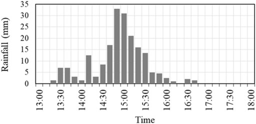
FIGURE 1. Rainfall hyetograph on June 14, 2015, at Gongguan rain gauge station (C1A760).

FIGURE 2

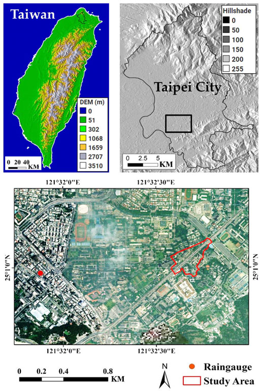
FIGURE 2. Study area (red polygon) at Gongguan, Taipei, Taiwan (the Google Earth images sourced from © Google, Landsat/Copernicus, and the shading image was derived from SRTM with 30 m resolution).

FIGURE 3

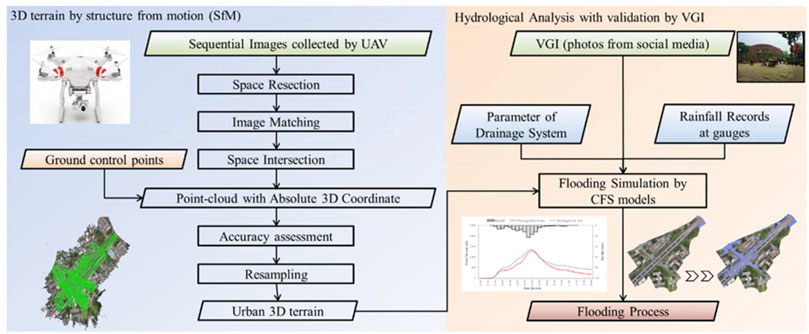
FIGURE 3. Conceptual flowchart of this study (the VGI photo was adopted from PTT, Taiwan).

DEM Generated by UAV

The procedure of developing the urban 3D terrain is shown on the left side of Figure 3. The methods of generating DEM from a set of aerial images or videos are quite mature (Zhou et al., 2004; Pollefeys et al., 2008), which are based on the fundamental principle of collinearity condition (Figure 4) expressed by the following equations:

$x_p=-f\left[\frac{m_{11}\left(X_P-X_L\right)+m_{12}\left(Y_P-Y_L\right)+m_{13}\left(Z_P-Z_L\right)}{m_{31}\left(X_P-X_L\right)+m_{32}\left(Y_P-Y_L\right)+m_{33}\left(Z_P-Z_L\right)}\right](1)$

$y_p=-f\left[\frac{m_{21}\left(X_P-X_L\right)+m_{22}\left(Y_P-Y_L\right)+m_{23}\left(Z_P-Z_L\right)}{m_{31}\left(X_P-X_L\right)+m_{32}\left(Y_P-Y_L\right)+m_{33}\left(Z_P-Z_L\right)}\right],(2)$

where $x_p$ and $y_p$ are the image coordinate of any point $p$; $X_P,Y_P,\text{ and }{Z}_P$ represent the ground coordinate of point p; $X_L,Y_L,\text{ and }{Z}_L$ represent ground coordinate of the projection (optical) center; $f$ is the focal length; $m_{11}\dots m_{33}$ are the coefficients of a $3\times 3$ rotation matrix defined by the angles $\omega$, $\varphi$, and $\kappa$ that transforms the ground coordinate system to the image coordinate system (Lillesand and Kiefer, 1999). The six parameters $X_L,Y_L,\text{ and }{Z}_L$ and $\omega$, $\varphi$, and $\kappa$ are used for exterior orientation of an image, which can be determined through the process of space resection, as illustrated in Figure 4. In the figure, the $X$, $Y$, and $Z$ coordinate of any point in the matched stereo pair of tilted images can be determined. Using a set of images taken by UAV, the ground coordinate of any point in the overlap of tilted images can be determined by the image matching method of structure from motion (Remondino and Fraser, 2006; Westoby et al., 2012). Finally, the coordinate accuracies at checkpoints are examined, and the urban 3D terrain model is obtained by resampling the coordinates to a regular gird system by the nearest neighboring method (Wu, 2013).

FIGURE 4

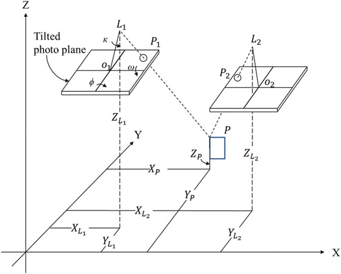
FIGURE 4. Illustration of collinearity condition and space intersection (adapted from Lillesand and Kiefer, 1999).

The UAV used in this study is DJI Phantom 2 Vision+ (Da-Jiang Innovations) which weighs 1.2 kg and has a camera with 4,384 × 2,466 pixels. The focal length of the camera is 3.3 mm, and the field-of-view is 110°. The UAV campaign was conducted in the early morning of July 22, 2015, in a cloudless condition from 06:00 to 06:40 to reduce the disturbances from weather and traffic. The camera on the UAV is set in a nadir-looking orientation for image data collection. In total, 589 positioned images were acquired with an overlap ratio of 75–85% and a mean spatial resolution of 2.84 cm. After space intersection, the average ground sampling distance of point cloud is 0.03 m. The UAV images were processed to generate orthomosaic image and digital surface model (DSM) with Pix4Dmapper Pro version 1.4.46 (Pix4D). To derive absolute coordinates, three ground control points (GCPs) were distributed in the study area (Figure 5). The coordinates of the three GCPs were acquired using the static positioning of the global navigation satellite system (GNSS) with positional accuracy at centimeter level. The absolute positions of the images captured through the GNSS receiver in the UAV were recorded to establish the coordinate system constrained on the three GCPs.

FIGURE 5

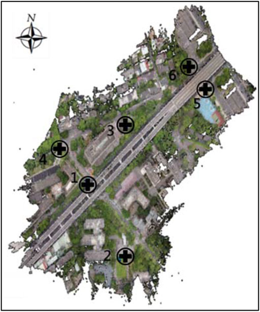
FIGURE 5. Images taken by UAV and the distribution of the ground control points.

The lens distortion of the camera was calibrated by flexible and powerful self-calibrating bundle adjustment (Remondino and Fraser, 2006). The calibration relies on the continuous overlapped images to do the aerotriangulation adjustment. After the interior orientation and the coordinates of the object points are calculated, the correction $\Delta x$ and $\Delta y$ can be revised as follows:

$\{\begin{array}{c}\mathrm{\Delta }x=-\mathrm{\Delta }{x}_0-\frac{x_i}{f}\mathrm{\Delta }f+K_1{x}_p{r}^2+K_2{x}_p{r}^4+K_3{x}_p{r}^6+P_1\left(r^2+2x_p^2\right)+2P_2{x}_p{y}_p\\ \mathrm{\Delta }y=-\mathrm{\Delta }{y}_0-\frac{y_i}{f}\mathrm{\Delta }f+K_1{y}_p{r}^2+K_2{y}_p{r}^4+K_3{y}_p{r}^6+P_2\left(r^2+2y_p^2\right)+2P_1{x}_p{y}_p\end{array},(3)$

where $\Delta f$ is the principal distance error; $\Delta x_0$ and $\Delta y_0$ are the displacements of the principal point; $K_1$, $K_2$, and $K_3$ are the parameters of the radial distortion; $P_1$ and $P_2$ are the parameters of the decentering distortion; and $r$ is the distance between the image point and the principal point. The calibrated parameters are listed in Table 1.

TABLE 1

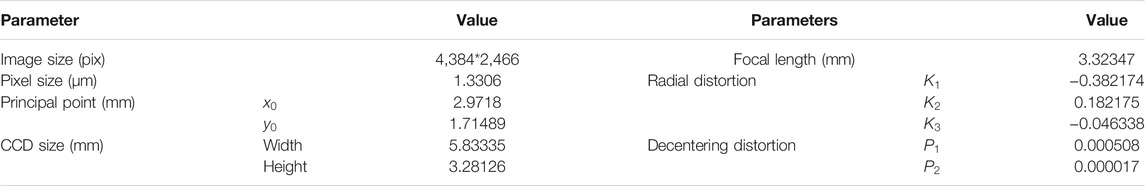
TABLE 1. Calibrated parameters for camera on the UAV.

For CFS application, the DSM was converted to DEM by removing the vegetation and the viaduct. The vegetation such as shrubs and grasses is detected by the normalized difference vegetation index (NDVI) in the range of 0.2–0.3 (Candiago et al., 2015). Since the UAV images only observed red, green, and blue bands, the near-infrared band was built on a specific linear combination of the three bands with a lower-pass filter (Rabatel et al., 2011). To remove the viaduct, the DSM points with elevations higher than 9 m on the Keelung Road are removed, and the DEMs beneath the viaduct were obtained through interpolation using the neighboring ground elevation data obtained by the UAV. This treatment did not deteriorate flood simulation because the area beneath the viaduct occupied about only 10% of the entire study domain, and the viaduct is located along the road centerline with higher ground elevations where floodwater less accumulated. Despite the viaduct, all the buildings are maintained so that flood simulation can more truly reflect the field conditions. Based on the NDVI and elevation thresholds, the vegetation and viaducts were filtered out in the DEM so that floodwater can transport smoothly on the ground surface. However, unlike traditional DEM, the elevations of buildings were not removed to reflect the blocking effect on water transverse.

VGI From Social Media

Ethical and legal concerns are big issues for collecting and using VGI (Foody et al., 2017). Fortunately, the Copyright Act and Relative Laws in Taiwan allow researchers to quote, within a reasonable scope, publicly released works for reports, comment, teaching, research, or other legitimate purposes (Intellectual Property Office., 2019). Based upon the act, the VGI data used in this study are collected from the most famous bulletin board system (BBS) in Taiwan named PTT. There are 8 photos collected from PTT posted during 15:20–16:30 on June 14, 2015. From these photos, we visually identified 8 locations in the study area, as shown in Figure 6. Since the VGI photos downloaded from social media were without EXIF attributes, an obvious landmark in each photo was identified to mark the GNSS and visually determine the relative flood depth with reference to neighboring objects with generally fixed size such as wheels of bikes or elevations of sidewalks. This GNSS information can be obtained based on post-disaster field surveys and is invariant as long as the landmarks were not destroyed during flooding. The time stamp and the virtual water depths in these photos were used to validate the CFS model. Although the time stamp when photos were posted on the internet may not always be the acquisition time and the flood depth estimated from photos may be subject to experts’ experience, these uncertainties can be reduced by the functions of “live stream” and “image recognition” on social media.

FIGURE 6

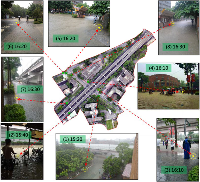
FIGURE 6. VGI photos from social media and their acquisition time (adopted from PTT, Taiwan).

CFS Model

The CFS model used in this study was developed by Jang et al. (2018), in which a 2D overland flow model (OFM) is coupled with a 1D sewer flow model (SFM) for sophisticated flood simulation in cities with drainage systems. The OFM and SFM are established based on shallow water equations and finite difference numerical methods. The alternate direction explicit scheme and implicit backward Euler algorithm are used to solve the OFM and SFM, respectively. The SFM adopted the Preissmann slot method (Cunge and Wegner, 1964) to calculate the full and partially full flow conditions at the same time. For the OFM simulation, the elevation at each grid center is extracted from the DEM data. During rain, the OFM is first initiated for surface water routing and the SFM is then initiated by the water that flows into the sewer pipes via street inlets. When the sewer pipes get full, the sewer water surcharges back onto the ground surface via manholes. In the simulation process, the water exchanged between the two models is determined by weir and orifice functions via a one-to-one relationship. To deal with wetting and drying, a tolerance water depth of 0.001 m is used to distinguish wet and dry cells. If a cell has a water depth lower than 0.001, all velocities in this cell are set to zero to ensure numerical stability caused by sudden drying in the next time step. The CFS model has been validated in urban and coastal areas with an overall hit rate of 0.8, meaning that 80% of the observed food extents are correctly predicted. The details of the CFS model can be referred to Jang et al. (2018); Jang et al. (2019).

Results and Discussions

DEM

The DEM accuracy is examined at the six GCPs. The errors in$X$, $Y$, and $Z$ directions range from −0.027 to 0.025 m, −0.055–0.061 m, and −0.024–0.026 m, respectively. The root mean square errors (RMSEs) of the absolute coordinate at the three GCPs are less than 0.053 m (Table 2). The RMSEs of SRTM were less than 10.343 m, and the RMSEs of 20 m DEM were less than 3.953 m. The comparison of the RMSE values showed that the UAV terrain model was with the smallest RMSE to achieve high precision topography. The orthoimage and the DEM resampled under spatial resolutions of 0.5, 5, 10, and 20 m are shown in Figure 7. In the figure, the elevation distributes from 5.5 to 55.8 m, and the buildings are displayed in warm colors.

TABLE 2

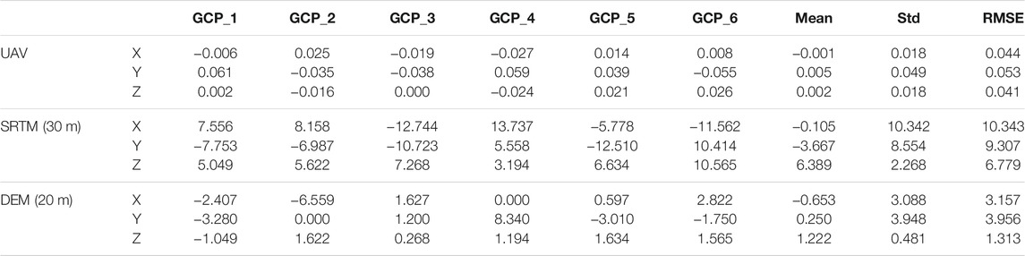
TABLE 2. Accuracy of the ground control points (m).

FIGURE 7

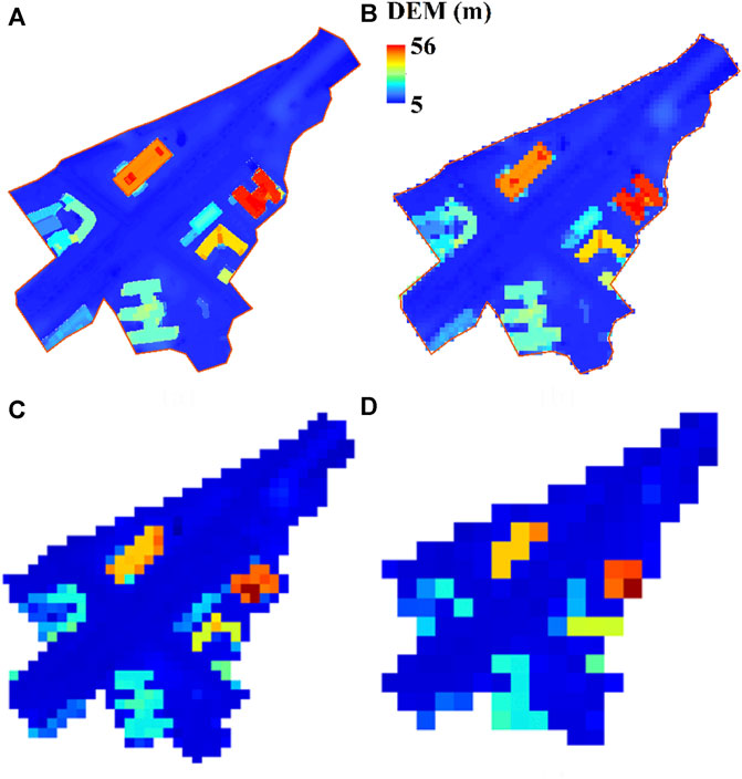
FIGURE 7. Resampled DEM with spatial resolution of (a) 0.5 m; (b) 5 m; (c) 10 m; (d) 20 m.

Flood Extent

To discover the influence of DEM resolution on flood simulation, the grid meshes of the CFS model are established under four grid sizes ($0.5\text{ m}\times 0.5\text{ m}$, $5\text{ m}\times 5\text{ m}$, $10\text{ m}\times 10\text{ m}$, $20\text{ m}\times 20\text{ m}$), in which the elevation at each grid center is extracted from the DEM with accordant resolution. The flood extents simulated under the four DEM resolutions at different times are displayed in Figure 8, in which the VGI points out of the 8 locations are marked if the simulated flood depths exceed 0.05 m. The value of 0.05 m is selected as the threshold because it is the shallowest water depth observed in the VGI photos (see point #6 in Figure 6). In the case with 0.5 m DEM resolution, flooding starts around 14:00 at points #4, #7, and #8, peaks around 15:00 at all points, and retreats at 17:00 back to original points. With coarser DEM resolutions, flooding occurs earlier and retreats later with more water trapped between buildings. When the grid resolutions increase to 10 and 20 m, the flood areas become more discontinuous with staggered distribution of wet and dry cells, and the flooding at points #1, #3, #5, and #6 are not predicted. Observing the flood maps between 15:00 and 18:00, water inundated on the rooftops of buildings can be properly simulated in the case with 0.5 m DEM resolution but not in the case with coarser resolutions.

FIGURE 8

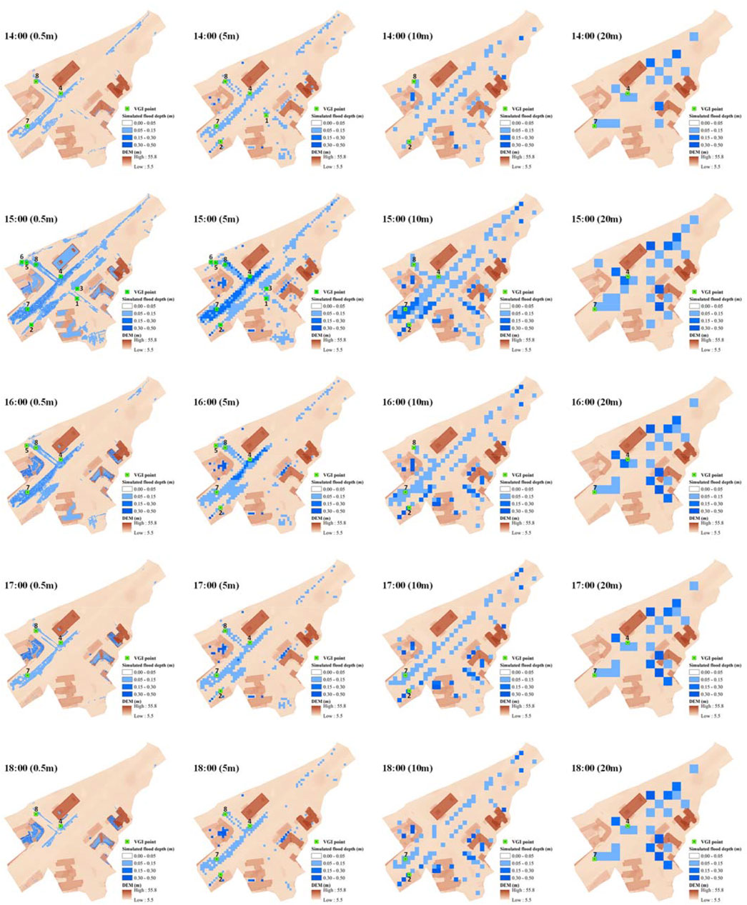
FIGURE 8. Simulated flood extents at different time under four DEM resolutions.

Flood Volume

The time series of flood volume simulated under the four DEM resolutions are displayed in Figure 9. Compared with the case with 0.5 m DEM resolution, the flood volume simulated under coarser DEM resolutions arises faster but descends slower with higher and earlier appearance of flood peak. This implies that when DEM resolution decreases, the topography becomes rugged, the friction increases, and the floodwater travels slower. The flood volumes for 10 and 20 m DEM resolutions are much larger than those for 0.5 and 5 m DEM resolutions, indicating that more water will be trapped in the depressions when the topography becomes more rugged. Table 3 compares the simulation and observation results in terms of flood occurrence time and water depth. The time stamps and estimated water depths (WD) are obtained from the VGI photos in Figure 6, and the flood durations at the eight VGI points when the water depth exceeds 0.05 m are determined based on the CFS results. It is seen that under 0.5 and 5 m DEM resolutions, the time stamps of VGI photos all lie within the simulated flood duration at the points with observed WD larger than 0.05 m (points #1, #2, #4, #7, and #8). At the rest points, the simulated and observed WDs are both smaller than 0.05 m. This good agreement between observation and simulation reveals that the flood model is accurate in rebuilding the process of flood transport under both DEM resolutions.

FIGURE 9

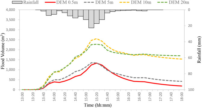
FIGURE 9. Comparison of simulated flood volume under four DEM resolutions.

TABLE 3

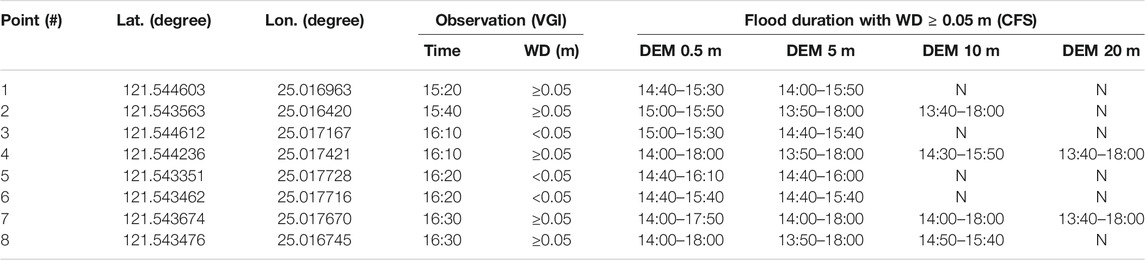
TABLE 3. Comparison between CFS and VGI results.

When the DEM resolutions become larger than 5 m, the periods with simulated WDs larger than 0.05 m do not coincide with the time stamps of VGI photos for 10 m DEM resolutions (at points #1 and #8) and 20 m DEM resolutions (at points #1, #2, and #8). Thus, the spatial resolution of DEM in urban areas should be at least finer than road width so that road profiles can be clearly displayed; otherwise, runoff transportation around buildings and on roads cannot be correctly simulated. The resolution of 5 m can be regarded as a threshold for flood modeling in urban areas, above which the geometries of buildings and roads cannot be clearly identified and the simulation performance deteriorates. Sub-meter resolution DEM data generated by UAVs are adequate for assessing the impact of localized flooding on transportation in cities. Some open-access topographic datasets, such as the 30 m resolution DEM by STRM from NASA (https://www2.jpl.nasa.gov/srtm/) and the open DEM in Taiwan with 20 m resolution (https://data.gov.tw/dataset/35430), are too coarse to serve the purpose.

Simulation Efficiency

Flood simulation under high grid resolutions is usually more time-consuming as compared to that under coarse grid resolutions due to the increase in grid numbers. The choice of grid resolution for flood simulation is a trade-off between accuracy and efficiency. For the study area in this research, there are 573,000 and 5,730 grids for the mesh with grid size 0.5 m and the mesh with grid size 5 m, which consumes 1,127 and 16 min of computational time, respectively (with Intel Core i7-7700 K CPU @ 4.2GHz and 64 GB RAM). For disaster emergency response on a regional scale, flood simulation under coarse grid resolution is enough to gain a fast and overall understanding of flood patterns. However, for evaluating the flood impact on critical infrastructures such as metro stations, power facilities, schools, government agencies, and hospitals, high-resolution flood simulation is required.

Conclusions

High-resolution flood simulation in an urban area is a challenging task since it requires high-resolution terrain and real-time flood information for model construction and validation. Aided by the rapidly growing technologies of remote sensing and crowdsourcing, it is possible to update DEM data and record the flood depth in real time by UAV and VGI. In this study, we adopt the UAV and VGI to sophisticate CFS modeling in the reconstruction of a flash flood event that occurred on 14 June 2015, in Taipei City. The CFS model is routed under four DEM resolutions with grid sizes 0.5, 5, 10, and 20 m separately. In the case with sub-meter DEM, the simulation results are in better agreement with the observation in terms of flood extent, depth, and occurrence. Using DEM with coarser resolutions (5, 10, and 20 m in this study) for CFS overestimates the flood duration on roads which may provide bias information to decision-makers for impact assessment on traffic and economic losses. The flood volume with 5 m DEM resolution shows a pattern similar to the finest resolution, whereas those with 10 and 20 m DEM resolutions have much higher flood peaks and more staggered distribution of wet and dry cells. The resolution of 5 m can be regarded as the optimum threshold for flood modeling in urban areas, coarser than which the simulation performance started to decline. Compared with traditional methods, the UAV and VGI are more economical and applicable in acquiring necessary data for high-resolution CFS.

Data Availability Statement

The raw data supporting the conclusion of this article will be made available by the authors, without undue reservation.

Author Contributions

J-HJ and Y-FS conceived the idea. Y-TL and J-HJ conducted the experiments and analyses. Y-FS, J-HJ, and Y-TL wrote the article. J-YH provided comments.

Funding

This work was funded by the Ministry of Science and Technology, Taiwan (Grant No. MOST 110-2625-M-006-006).

Conflict of Interest

The authors declare that the research was conducted in the absence of any commercial or financial relationships that could be construed as a potential conflict of interest.

Publisher’s Note

All claims expressed in this article are solely those of the authors and do not necessarily represent those of their affiliated organizations, or those of the publisher, the editors, and the reviewers. Any product that may be evaluated in this article, or claim that may be made by its manufacturer, is not guaranteed or endorsed by the publisher.

Acknowledgments

The authors would like to thank the Central Weather Bureau and the National Science and the Technology Center for Disaster Reduction for providing research data.

References

Bao, J., Sherwood, S. C., Alexander, L. V., and Evans, J. P. (2017). Future Increases in Extreme Precipitation Exceed Observed Scaling Rates. Nat. Clim Change 7, 128–132. doi:10.1038/nclimate3201

CrossRef Full Text | Google Scholar

Busuioc, A., Baciu, M., Breza, T., Dumitrescu, A., Stoica, C., and Baghina, N. (2017). Changes in Intensity of High Temporal Resolution Precipitation Extremes in Romania: Implications for Clausius-Clapeyron Scaling. Clim. Res. 72, 239–249. doi:10.3354/cr01469

CrossRef Full Text | Google Scholar

Candiago, S., Remondino, F., De Giglio, M., Dubbini, M., and Gattelli, M. (2015). Evaluating Multispectral Images and Vegetation Indices for Precision Farming Applications from UAV Images. Remote Sensing 7 (4), 4026–4047. doi:10.3390/rs70404026

CrossRef Full Text | Google Scholar

Cervone, G., Sava, E., Huang, Q., Schnebele, E., Harrison, J., and Waters, N. (2015). Using Twitter for Tasking Remote-Sensing Data Collection and Damage Assessment: 2013 Boulder Flood Case Study. Int. J. Remote Sensing 37 (1), 100–124. doi:10.1080/01431161.2015.1117684

CrossRef Full Text | Google Scholar

Chan, S. C., Kendon, E. J., Roberts, N. M., Fowler, H. J., and Blenkinsop, S. (2016). The Characteristics of Summer Sub-hourly Rainfall over the Southern UK in a High-Resolution Convective Permitting Model. Environ. Res. Lett. 11, 094024. doi:10.1088/1748-9326/11/9/094024

CrossRef Full Text | Google Scholar

Chang, T.-J., Wang, C.-H., and Chen, A. S. (2015). A Novel Approach to Model Dynamic Flow Interactions between Storm Sewer System and Overland Surface for Different Land Covers in Urban Areas. J. Hydrol. 524, 662–679. doi:10.1016/j.jhydrol.2015.03.014

CrossRef Full Text | Google Scholar

Cunge, J. A., and Wegner, M. (1964). Intégration numérique des équations d'écoulement de barré de Saint-Venant par un schéma implicite de différences finies. La Houille Blanche 50, 33–39. doi:10.1051/lhb/1964002

CrossRef Full Text | Google Scholar

Foody, G., See, L., Fritz, S., Mooney, P., Olteanu-Raimond, A-M., Fonte, C. C., et al. (2017). Mapping and the Citizen Sensor. London: Ubiquity Press. doi:10.5334/bbf.License

CrossRef Full Text | Google Scholar

Fu, J.-C., Huang, H.-Y., Jang, J.-H., and Huang, P.-H. (2019). River Stage Forecasting Using Multiple Additive Regression Trees. Water Resour. Manage. 33, 4491–4507. doi:10.1007/s11269-019-02357-x

CrossRef Full Text | Google Scholar

Goodchild, M. F., and Glennon, J. A. (2010). Crowdsourcing Geographic Information for Disaster Response: A Research Frontier. Int. J. Digital Earth 3, 231–241. doi:10.1080/17538941003759255

CrossRef Full Text | Google Scholar

Huang, X., Wang, C., Li, Z., and Ning, H. (2018). A Visual-Textual Fused Approach to Automated Tagging of Flood-Related Tweets during a Flood Event. Int. J. Digital Earth 12, 1248–1264. doi:10.1080/17538947.2018.1523956

CrossRef Full Text | Google Scholar

Hunter, N. M., Bates, P. D., Horritt, M. S., and Wilson, M. D. (2007). Simple Spatially-Distributed Models for Predicting Flood Inundation: A Review. Geomorphology 90 (3–4), 208–225. doi:10.1016/j.geomorph.2006.10.021

CrossRef Full Text | Google Scholar

Intellectual Property Office (2019). Ministry of Economic Affairs. Copyright Act 2016 https://www.tipo.gov.tw/public/Attachment/71417531682.pdf (Accessed September 26, 2019).

Google Scholar

Jahanbazi, M., and Egger, U. (2014). Application and Comparison of Two Different Dual Drainage Models to Assess Urban Flooding. Urban Water J. 11, 584–595. doi:10.1080/1573062X.2013.871041

CrossRef Full Text | Google Scholar

Jang, J.-H., Chang, T.-H., and Chen, W.-B. (2018). Effect of Inlet Modelling on Surface Drainage in Coupled Urban Flood Simulation. J. Hydrol. 562, 168–180. doi:10.1016/j.jhydrol.2018.05.010

CrossRef Full Text | Google Scholar

Jang, J.-H., Hsieh, C.-T., and Chang, T.-H. (2019). The Importance of Gully Flow Modelling to Urban Flood Simulation. Urban Water J. 16 (5), 377–388. doi:10.1080/1573062X.2019.1669198

CrossRef Full Text | Google Scholar

Jang, J.-H., Vohnicky, P., and Kuo, Y.-L. (2021). Improvement of Flood Risk Analysis via Downscaling of hazard and Vulnerability Maps. Water Resour. Manage. 35, 2215–2230. doi:10.1007/s11269-021-02836-0

CrossRef Full Text | Google Scholar

Kim, Y. D., Tak, Y. H., Park, M. H., and Kang, B. (2020). Improvement of Urban Flood Damage Estimation Using a High‐resolution Digital Terrain. J. Flood Risk Management 13 (Suppl. 1), e12575. doi:10.1111/jfr3.12575

CrossRef Full Text | Google Scholar

Komolafe, A. A., Herath, S., and Avtar, R. (2018). Sensitivity of Flood Damage Estimation to Spatial Resolution. J. Flood Risk Manage. 11, S370–S381. doi:10.1111/jfr3.12224

CrossRef Full Text | Google Scholar

Kuiry, S. N., Sen, D., and Bates, P. D. (2010). Coupled 1D-Quasi-2d Flood Inundation Model with Unstructured Grids. J. Hydraul. Eng. 136, 493–506. doi:10.1061/(ASCE)HY.1943-7900.0000211

CrossRef Full Text | Google Scholar

Le Coz, J., Patalano, A., Collins, D., Guillén, N. F., García, C. M., Smart, G. M., et al. (2016). Crowdsourced Data for Flood Hydrology: Feedback from Recent Citizen Science Projects in Argentina, France and New Zealand. J. Hydrol. 541, 766–777. doi:10.1016/j.jhydrol.2016.07.036

CrossRef Full Text | Google Scholar

Leitão, J. P., Boonya-aroonnet, S., Prodanović, D., and Maksimović, Č. (2009). The Influence of Digital Elevation Model Resolution on Overland Flow Networks for Modelling Urban Pluvial Flooding. Water Sci. Technol. 60 (12), 3137–3149. doi:10.2166/wst.2009.754

PubMed Abstract | CrossRef Full Text | Google Scholar

Leitão, J. P., Moy de Vitry, M., Scheidegger, A., and Rieckermann, J. (2016). Assessing the Quality of Digital Elevation Models Obtained from Mini Unmanned Aerial Vehicles for Overland Flow Modelling in Urban Areas. Hydrol. Earth Syst. Sci. 20, 1637–1653. doi:10.5194/hess-20-1637-2016

CrossRef Full Text | Google Scholar

Li, J., and Wong, D. W. S. (2010). Effects of DEM Sources on Hydrologic Applications. Comput. Environ. Urban Syst. 34, 251–261. doi:10.1016/j.compenvurbsys.2009.11.002

CrossRef Full Text | Google Scholar

Lillesand, T. M., and Kiefer, R. W. (1999). Remote Sensing and Image Interpretation. 4th Ed. New York: Wiley.

Google Scholar

Michelsen, N., Dirks, H., Schulz, S., Kempe, S., Al-Saud, M., and Schüth, C. (2016). Youtube as a Crowd-Generated Water Level Archive. Sci. Total Environ. 568, 189–195. doi:10.1016/j.scitotenv.2016.05.211

PubMed Abstract | CrossRef Full Text | Google Scholar

Panthou, G., Vischel, T., and Lebel, T. (2014). Recent Trends in the Regime of Extreme Rainfall in the Central Sahel. Int. J. Climatol. 34, 3998–4006. doi:10.1002/joc.3984

CrossRef Full Text | Google Scholar

Pollefeys, M., Nistér, D., Frahm, J.-M., Akbarzadeh, A., Mordohai, P., Clipp, B., et al. (2008). Detailed Real-Time Urban 3D Reconstruction from Video. Int. J. Comput. Vis. 78, 143–167. doi:10.1007/s11263-007-0086-4

CrossRef Full Text | Google Scholar

Pregnolato, M., Ford, A., Wilkinson, S. M., and Dawson, R. J. (2017). The Impact of Flooding on Road Transport: A Depth-Disruption Function. Transportation Res. D: Transport Environ. 55, 67–81. doi:10.1016/j.trd.2017.06.020

CrossRef Full Text | Google Scholar

Rabatel, G., Gorretta, N., and Labbé, S. (2011). “Getting NDVI Spectral Bands from a Single Standard RGB Digital Camera: A Methodological Approach,”. Advances in Artificial Intelligence. CAEPIA 2011. Lecture Notes in Computer Science. Editors J. A. Lozano, J. A. Gámez, and J. A. Moreno (Berlin, Heidelberg: La Laguna, Spain: Springer), 7023, 333–342. doi:10.1007/978-3-642-25274-7_34

CrossRef Full Text | Google Scholar

Remondino, F., and Fraser, C. (2006). Digital Camera Calibration Methods: Considerations and Comparisons. Int. Arch. Photogramm. Remote Sens. Spat. Inf. Sci. 36, 266–272. http://citeseerx.ist.psu.edu/viewdoc/download?doi=10.1.1.67.

Google Scholar

Saksena, S., and Merwade, V. (2015). Incorporating the Effect of DEM Resolution and Accuracy for Improved Flood Inundation Mapping. J. Hydrol. 530, 180–194. doi:10.1016/j.jhydrol.2015.09.069

CrossRef Full Text | Google Scholar

Sankey, T. T., McVay, J., Swetnam, T. L., McClaran, M. P., Heilman, P., and Nichols, M. (2018). UAV Hyperspectral and Lidar Data and Their Fusion for Arid and Semi‐arid Land Vegetation Monitoring. Remote Sens Ecol. Conserv 4, 20–33. doi:10.1002/rse2.44

CrossRef Full Text | Google Scholar

Seyoum, S. D., Vojinovic, Z., Price, R. K., and Weesakul, S. (2012). Coupled 1D and Noninertia 2D Flood Inundation Model for Simulation of Urban Flooding. J. Hydraul. Eng. 138, 23–34. doi:10.1061/(ASCE)HY.1943-7900.0000485

CrossRef Full Text | Google Scholar

Starkey, E., Parkin, G., Birkinshaw, S., Large, A., Quinn, P., and Gibson, C. (2017). Demonstrating the Value of Community-Based ('citizen Science') Observations for Catchment Modelling and Characterisation. J. Hydrol. 548, 801–817. doi:10.1016/j.jhydrol.2017.03.019

CrossRef Full Text | Google Scholar

Suarez, P., Anderson, W., Mahal, V., and Lakshmanan, T. R. (2005). Impacts of Flooding and Climate Change on Urban Transportation: A Systemwide Performance Assessment of the Boston Metro Area. Transportation Res. Part D: Transport Environ. 10, 231–244. doi:10.1016/j.trd.2005.04.007

CrossRef Full Text | Google Scholar

Tauro, F., Selker, J., van de Giesen, N., Abrate, T., Uijlenhoet, R., Porfiri, M., et al. (2018). Measurements and Observations in the XXI century (MOXXI): Innovation and Multi-Disciplinarity to Sense the Hydrological Cycle. Hydrological Sci. J. 63, 169–196. doi:10.1080/02626667.2017.1420191

CrossRef Full Text | Google Scholar

Vaze, J., Teng, J., and Spencer, G. (2010). Impact of DEM Accuracy and Resolution on Topographic Indices. Environ. Model. Softw. 25, 1086–1098. doi:10.1080/01431160020993110.1016/j.envsoft.2010.03.014

CrossRef Full Text | Google Scholar

Westoby, M. J., Brasington, J., Glasser, N. F., Hambrey, M. J., and Reynolds, J. M. (2012). 'Structure-from-Motion' Photogrammetry: A Low-Cost, Effective Tool for Geoscience Applications. Geomorphology 179, 300–314. doi:10.1016/j.geomorph.2012.08.021

CrossRef Full Text | Google Scholar

Wu, C. (2013). “Towards Linear-Time Incremental Structure from Motion,” in International Conference on 3D Vision-3DV 2013 (WA, USA: IEEE), 127–134. doi:10.1109/3dv.2013.25

CrossRef Full Text | Google Scholar

Yang, P., Ames, D. P., Fonseca, A., Anderson, D., Shrestha, R., Glenn, N. F., et al. (2014). What Is the Effect of LiDAR-Derived DEM Resolution on Large-Scale Watershed Model Results? Environ. Model. Softw. 58, 48–57. doi:10.1016/j.envsoft.2014.04.005

CrossRef Full Text | Google Scholar

Yang, P., Ren, G., and Yan, P. (2017). Evidence for a strong Association of Short-Duration Intense Rainfall with Urbanization in the Beijing Urban Area. J. Clim. 30, 5851–5870. doi:10.1175/JCLI-D-16-0671.1

CrossRef Full Text | Google Scholar

Yin, J., Yu, D., Yin, Z., Liu, M., and He, Q. (2016). Evaluating the Impact and Risk of Pluvial Flash Flood on Intra-urban Road Network: A Case Study in the City center of Shanghai, China. J. Hydrol. 537, 138–145. doi:10.1016/j.jhydrol.2016.03.037

CrossRef Full Text | Google Scholar

Zhou, G., Song, C., Simmers, J., and Cheng, P. (2004). Urban 3D GIS from LiDAR and Digital Aerial Images. Comput. Geosciences 30, 345–353. doi:10.1016/j.cageo.2003.08.012

CrossRef Full Text | Google Scholar