Water Resource Availability Assessment Through Hydrological Simulation Under Climate Change in the Huangshui Watershed of the Qinghai–Tibet Plateau

The related dynamic change in meteorological and hydrological parameters is critical for available water resources, development management options, and making informed decisions. In this study, to enhance the resolution of the predicted meteorological and hydrological parameters under climate change, the statistical downscaling method (SDSM), the generalized regression neural network (GRNN) model, the Soil and Water Assessment Tool (SWAT) model, and the improved Tennant method were integrated into a framework. The available water resources were assessed in the Huangshui watershed of the Qinghai–Tibet Plateau, which has the highest average elevation in the world. The meteorological parameters were obtained by the SDSM model and the GRNN model. The SWAT model used the meteorological parameters to simulate the hydrological data under climate change scenarios. Considering the meteorological conditions and the high sediment content in the basin, the available water resources are evaluated by the improved Tennant method. The meteorological data of the Xining station from 1958 to 2011 were used to analyze the dynamic changes and mutation trends in the data. The results indicated that the precipitation would have a great increase during the wet season from May to September, and the flows and available water resources would decrease with increasing carbon emissions under different representative concentration pathways (RCPs).

1 Introduction

The spatial and temporal dynamics of ecosystems are closely related to fluctuations in the climate. The meteorological parameters are severely affected by the climate change that cause the reallocation of water resources and lead to crisis of water utilization and threaten human lives (Song et al., 2019; Sharma and Goyal, 2020). In addition, as sensitive climate and ecosystem area, the meteorological data in the ecotone attracts major concern for fragile ecosystem management. The climate changes are expected to produce large shifts in water distributions at unprecedented rates (Hanewinkel et al., 2013; Teng et al., 2020). Thus, predicting the meteorological parameters, the hydrological parameters, and the water resource availability in the ecotone areas under different climate change scenarios is important for planning and managing the ecological environment.

Previously, in order to meet the actual condition in regional scale, the downscaling methods were developed for improving the spatial resolution of the global climate models (GCMs) in climate change impact assessment (Thuiller et al., 2005; Delworth, 2006; Taylor et al., 2012; Hughes and Mazibuko, 2018). Among those methods, due to its relatively low computational requirements, the functional transformation downscaling method is the most commonly used downscaling method (Ghosh and Mujumdar, 2008; Guo et al., 2014). For example, Jeong et al. (2012) provided a multisite hybrid statistical downscaling procedure combining regression-based and stochastic weather generation approaches for multisite simulations of daily precipitation. Piras et al. (2015) advanced a statistical downscaling method to analyze the impacts of climate change on precipitation and discharges in a Mediterranean basin. Tang et al. (2016) developed statistical and dynamical downscaling methods to simulate the surface climate of China based on large-scale information from either reanalysis data or global climate models. Although the large-scale parameters, such as the atmospheric oscillation and the circulation patterns with slowly changing processes and low resolutions can be addressed by the downscaling process, the changing process of small-scale parameters (e.g., local temperature and precipitation) are needed to reflect for analyzing the response relationship between underlying surfaces and meteorological factors in hydrological simulations (Sillmann et al., 2013; Friedlingstein et al., 2014; Zhang et al., 2020).

Moreover, water resource availability refers to the largest one-time utilization quantity of local water resources within an expected time range under deduction of the ecological water demand, and the determination of ecological water demand is the key to evaluating water resource availability (Kattsov et al., 2007; Whitehead et al., 2009). The acceptable approaches to simulate ecological water demand can be divided into four categories, including the hydrological index method, hydraulic method, holistic method, and habitat method. Among these, as a typical representative of hydrological index measures, the Tennant method is widely used due to its convenient operation and high accuracy to determine the ratio of the ecological water demand to the average annual natural flow through the correlation between the flow in rivers and environmental quality of fish habitats (Yakup et al., 2018; Suwal et al., 2020; Joseph et al., 2021). However, the application of the Tennant method for permanent rivers in arid and semiarid areas still has some limitations. The Tennant method divides the year into two periods to calculate the recommended average percentage of runoff according to the amount of runoff monthly. At the same time, this method is mainly studied on the basis of considering the impact of runoff on fish and ecosystem, so it needs to be adjusted in the study area with high sediment content in rivers. So, it needs to be improved according to the actual situation and regional characteristics.

Therefore, in consideration of the above limitation, the aim of this study is to develop a general framework through integration with the SDSM downscaling method, the GRNN model, the SWAT model, and the Tennent method for a comprehensive meteorological and hydrographic prediction, and available water resource assessment of the Huangshui watershed in the Qinghai–Tibet Plateau with the fragile ecological environment. For the framework, the SDSM downscaling method was applied for temperature prediction according to the large-scale observed meteorological data, and the GRNN model was advanced to improve the prediction accuracy of monthly precipitation. The predicted temperature and precipitation values were the main input parameters to the SWAT model to simulate more precise hydrologic data under different climate change scenarios, and the water availability within basin scale can be further obtained through the improvement of the Tennent method. The study results could analyze the available water resource for generating effective water resource management schemes and address the impacts of the climate change on ecotones in the basin.

2 Methodology

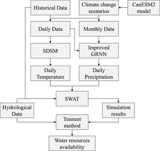
This study constructed a comprehensive assessment framework of water resource availability based on hydrological simulation under the impact of climate change. The methodology contains three parts. The first step is the development of future climate conditions including daily temperature with the SDSM method (Section 2.1) and precipitation with the GRNN model (Section 2.2). The second step involves using the downscaled daily precipitation and temperature to simulate daily runoff using the SWAT model (Section 2.3). The third step involves using the hydrological data to calculate the water resource availability using the Tennant method (Section 2.4). To evaluate the SDSM model, the GRNN model, and the SWAT model, R2 and NSE are used (Section 2.5). Figure 1 presents the general framework of the evaluation method of available water resources based on hydrological simulation under the impact of climate change. Historical data and climate change scenarios both include daily and monthly data. The daily data of historical data and climate change scenarios will be used to predict temperature through the SDSM model. The daily data and monthly data of historical data and climate change scenarios are used by the GRNN model, and the precipitation prediction results will be obtained.

FIGURE 1

FIGURE 1. The framework of evaluation method of available water resources.

2.1 Statistical Downscaling Model

Statistical downscaling model (SDSM) is an effective decision supporting tool with a robust statistical downscaling technique for assessing local climate change impacts (Wilby et al., 2002; Meenu et al., 2013). Under the present and future climate forcing, this model can facilitate the rapid development of the multiple, low-cost, and single-site scenarios of daily surface weather variables. The general equation for the SDSM is as follows:

$R=F\left(L\right)(1)$

where R = predictand (a local climate variable), L = predictor (a set of large-scale climate variables), and F = deterministic/stochastic function conditioned by L and is estimated empirically from historical observations.

Statistical downscaling model (SDSM) is used to downscale temperature factor, which includes the daily maximum and minimum temperatures. The data required include the daily measured data of weather station and the daily large-scale meteorological data obtained by GCM. In order to achieve the purpose of this study, the software (SDSM v. 5.2) was used.

2.2 Generalized Regression Neural Network Model

Considering that the SDSM is not accurate enough for daily precipitation prediction, we built a new generalized regression neural network model (GRNN method) to predict precipitation, and the new method is suitable for the description of various nonlinear relations. This method is based on nonparametric regression. It takes the sample data as a posteriori condition, performs nonparametric estimation, and calculates the network output according to the maximum probability principle (Specht, 1991; Dalkilic et al., 2014). At present, it has been applied in many fields such as control decision system, structure analysis, and so on (Kumar and Malik, 2016). The network has the following obvious advantages: 1) No model parameters need to be trained, and the convergence speed is fast; 2) Based on radial basis function network, it has good nonlinear approximation performance, and has good adaptability to curve fitting problem. In this model, a network can be employed to estimate a dependent variable from an independent variable through finite datasets (Cigizoglu and Alp, 2006). The theoretical foundation of the GRNN model is the kernel regression, which is a nonlinear regression analysis. The regression of the random variable y on the observed values X of random variable x can be found using:

$E\left(y\mathrm{|}X\right)=\frac{{\displaystyle {\int }_{-\infty }^{0}yf\left(X,y\right)dy}}{{\displaystyle {\int }_{-\infty }^{0}f\left(X,y\right)dy}}(2)$

where $f\left(X,y\right)$ is a known joint continuous probability density function. When $f\left(X,y\right)$ is unknown, it should be estimated from a set of observations of x and y. $f\left(X,y\right)$ can be estimated using the nonparametric consistent estimator suggested as follows:

$\stackrel{⌢}{f}\left(X,Y\right)=\frac{1}{\left(2\pi \right)\frac{\rho +1}{2}{\sigma }^{\rho +1}}\frac{1}{n}{\displaystyle \sum _{i=1}^n\exp \left[-\frac{{\left(X-X^i\right)}^T\left(X-X^i\right)}{2{\sigma }^2}\right]\exp \left[-\frac{{\left(Y-Y^i\right)}^2}{2{\sigma }^2}\right]}(3)$

where n = sample size, $\rho$ = dimensionality of random variable x, and $\sigma$ = smooth parameter.

By substituting Eq. 3 into Eq. 2, and after solving the integration, the following equation will be obtained:

$\stackrel{⌢}{Y}\left(X\right)=\frac{{\displaystyle \sum _{i=1}^{n}y\exp \left[-\frac{{\left(X-X^i\right)}^T\left(X-X^i\right)}{2{\sigma }^2}\right]}}{{\displaystyle \sum _{i=1}^n\exp \left[-\frac{{\left(X-X^i\right)}^T\left(X-X^i\right)}{2{\sigma }^2}\right]}}(4)$

Equation 4 is directly applicable to the issues involving numerical data. In order to improve the predictive accuracy caused by the nontemporality of daily precipitation, the GRNN model was improved to construct a two-layer GRNN model as shown in Figure 2. First, the first layer of the GRNN model is constructed, in which the monthly precipitation is predicted by multiple monthly scale factors. Second, the second-level GRNN model is constructed, which uses multiple daily scale factors and monthly precipitation as input variables and daily precipitation as output variables to calibrate and verify the model. The model is composed of the two layers models. Through the gradual simulation and prediction, the nonlinear relationship between the large-scale meteorological data and the measured daily precipitation is obtained.

FIGURE 2

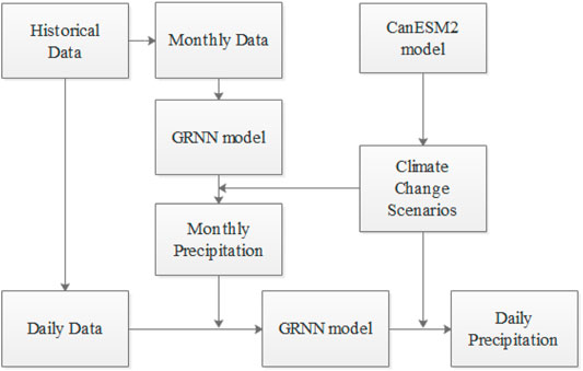
FIGURE 2. The improved precipitation prediction model based on the generalized regression neural network (GRNN) model.

2.3 Hydrological Model

The Soil and Water Assessment Tool (SWAT) is a physically based semi-distributed hydrological model used to simulate the quantity and quality of surface water and can be also used to predict the impact of land use, land management practices, and climate change on hydrology (Arnold et al., 2012), and developed by the Agricultural Research Service (ARS) of the United States Department of Agriculture (USDA). The hydrological simulation in the SWAT model is mainly carried out through the hydrological module. The process is divided into two parts, land slope runoff and river channel runoff. The land slope runoff consists of precipitation process, rainwater trapped by plant canopy into soil, groundwater, and surface runoff (Nyika et al., 2020). The river channel runoff is mainly affected by the evaporation of water and infiltration of the river water. The balance equation of water quantity in this model is shown as follows:

$S{W}_t=S{W}_0+{\displaystyle \sum _{i=1}^t\left(R_{day}-Q_{surf}-E_a-W_{seep}-Q_{gw}\right)}(5)$

where $S{W}_t$ = ultimate soil moisture content, $S{W}_0$ = antecedent soil moisture content, $t$ = sample size, $R_{day}$ = daily total precipitation, $Q_{surf}$ = total surface runoff, $E_a$ = the total evapotranspiration, $W_{seep}$ = soil infiltration capacity and lateral flow volume, and $Q_{gw}$ = total underground runoff.

2.4 Tennant Method of Water Resource Availability Assessment

The Tennant method is an operational method originated from the midwest of the United States, which can determine the ratio of ecological water demand in the average annual river flow and evaluate the degree of river ecology according to the analysis of the relationship between the flow of multiple rivers and the environmental quality of fish habitat (Abbaspour et al., 2007; Ateeq-Ur and Abdul, 2018). Specifically, 10% of the average flow is a minimum instantaneous flow recommended to sustain short-term survival habitat for most aquatic life forms, 30% of the average flow is recommended as a base flow to sustain standard survival conditions for most aquatic life forms, and 60% of the average flow provides the excellent habitat for most aquatic life forms. In addition, according to the monthly runoff changes and the growth conditions of fish and other aquatic organisms, the evaluation standard can also be divided into two periods from October to March and April to September. The Tennant method can be used in calculating the ecological water demand in permanent arid and semi-arid rivers. Practically, some appropriate improvements should be conducted based on the actual hydrological changes and the regional characteristics. In this study, as the largest tributary of the upper reaches of the Yellow River, the Huangshui River Basin suffered from serious soil erosion and high sediment content due to the influence of geological conditions and human factors. The sediment is mainly concentrated from June to September. Through the calculation of the average sediment transport in Xining station, the average sediment concentration is 2.45 kg/m³. Therefore, in order to ensure that there are enough water resources in the Huangshui River to transport the sediment in the water to the downstream, it is necessary to increase the sediment transport water demand on the basis of the original Tennant method.

2.5. Model performance evaluation method

In this study, the determination coefficient (R²) and Nash–Sutcliffe efficiency coefficient (NSE) were used to evaluate the accuracy of the simulation results. The formulas are shown as follows:

$R^2=\frac{{\left[{\displaystyle \sum _{i=1}^n\left(O_i-\overline{O}\right)\left(S_i-\overline{S}\right)}\right]}^2}{{\displaystyle \sum _{i=1}^n{\left(O_i-\overline{O}\right)}^2}{\displaystyle \sum _{i=1}^n{\left(S_i-\overline{S}\right)}^2}}(6)$

$NSC=1-\frac{{\displaystyle {\sum }_{i=1}^n{\left(S_i-O_i\right)}^2}}{{\displaystyle {\sum }_{i=1}^n{\left(O_i-\overline{O}\right)}^2}}(7)$

where, $i$ = the number of time series, $i=\mathrm{1,2...},n$; $S_i$ = the ith modeled value; $O_i$ = the ith observation; $\overline{S}$ = the average of modeled values; and $\overline{O}$ = the average of observations. R² ranges from 0 to 1. The NSE ranges from minus infinity to 1.

3 Study Area and Data

3.1 Overview of the Huangshui Watershed

The Huangshui watershed, a semi-arid area with an average annual precipitation of less than 400 mm, is located in the upstream of the Yellow River. Moreover, this area is the core region of the Tibetan Plateau with the most dense population and the most developed economy. Therefore, as a transitional and ecologically fragile zone between the Tibetan Plateau and the Loess Plateau, this area has become a globally well-known ecologically vulnerable area with the characteristics of high ecological sensitivity, low environmental capacity, a weak capability to withstand interference, and poor stability (Song et al., 2009; Chen et al., 2015).

The Huangshui watershed has a total area of 10,337 km², and the overall terrain of the basin is high in the northwest and low in the southeast. The river originates from the mountains at an elevation of 4,300 m, and the total basin has elevations ranging from 2,100 to 5,000 m. The terrain of the river basin is complex and diverse, mainly including mountains, hills, valley basins, and other landforms. The upper reaches of the river are mainly canyons, while the middle and lower reaches are mainly wider canyons. The study area is located in the inland plateau continental climate, and belongs to a subhumid climate area. The area has a high elevation, a large amount of evaporation, and large temperature differences between day and night. The annual precipitation is unevenly distributed in this region, and 60%–80% of the total precipitation is concentrated in the rainy season. Moreover, the dry season from November to February only accounts for approximately 3% of the annual precipitation. In addition, the river networks are arranged in dense, branching patterns, with more than 10 main tributaries.

3.2 Data Collection

The meteorological data were obtained from the standard weather station of the Yellow River upstream (1952–2011), which was provided by the “Comprehensive data platform of Ningxia-Inner Mongolia Reach of the Yellow River,” National Key Basic Research Program of China. These data were measured on a daily time span, and the original format was “.txt.” The data of the Menyuan meteorological station (W1) and Xining meteorological station (W2) are used in this study. The study data contained daily meteorological data for the upper reaches of the Yellow River and its surrounding areas from 1952 to 2011. The standard station data included air pressures, temperatures, humidity values, wind speeds, and 15 other factors.

The large-scale meteorological data obtained by GCM used to estimate the future trends in climate change came from the CanESM2 model (the second-generation Canadian Earth System Model), which was developed by CCCma (Canadian Centre for Climate Modeling and Analysis). The selected large-scale meteorological factors include the daily maximum near-surface air temperature (tasmax), daily minimum near-surface air temperature (tasmin), near-surface air temperature (tas), precipitation (pr), near-surface relative humidity (ths), surface air pressure (ps), total cloud fraction (clt), eastward near-surface wind (uas), and northward near-surface wind (vas). The data used in this study were based on CMIP5 (Coupled Model Intercomparison Project Phase 5), which included the historical scenario, RCP (representative concentration pathway) 2.6 scenario, RCP4.5 scenario, and RCP8.5 scenario (Park et al., 2018). These data had two kinds of time spans: daily and monthly. The original format was “.nc,” and the data were spatial grid data with a spatial resolution of 2.5°.

The DEM (digital elevation model) was provided by the Geospatial Data Cloud site, Computer Network Information Center, Chinese Academy of Sciences (http://www.gscloud.cn/sources/accessdata/310?pid=302). The data were derived from the ASTER GDEM dataset based on the Advanced Spaceborne Thermal Emission and Reflectance Radiometer (ASTER) data developed by the National Aeronautics and Space Administration (NASA) and the Ministry of Economy, Trade, and Industry (METI) of Japan. The resolution of the DEM data used was 30 m, and the original format was “.tiff.” Based on Landsat 8 remote-sensing images, the datasets were generated by manual visual interpretation. In the study area, the land use types included the cultivated land, forestland, grassland, water area, residential land, and unused land. These data were obtained from the data center of resources and environment science, Chinese Academy of Sciences and are 1-km resolution, remote-sensing monitoring data of the land use status of China in 2015 with the “.tiff” format. According to the analysis, grassland, forestland, and cultivated land were the main types in this region, accounting for 52.45, 20.82, and 18.02%, respectively. Construction land accounted for only 3.22% of the total area. The soil parameters were provided by the China Soil Map Based Harmonized World Soil Database (HWSD). The soil data were provided by the Nanjing Soil Institute for the second land survey in 1995, and the data resolution was 1 km with the “.tiff” format. Considering that the soil particle size grading standard in the HWSD is American standard, these data can be directly used to establish the SWAT model soil database. The division threshold was set at 2,000 ha, and the Xiaoxiaqiao section was selected as the outlet of the watershed. A total of 305 subbasins are generated, and the final division results are shown in Figure 3D. Figures 3A–D have been used in the SWAT model, and they are elevation, land use type, soil type, and subwatershed distribution.

FIGURE 3

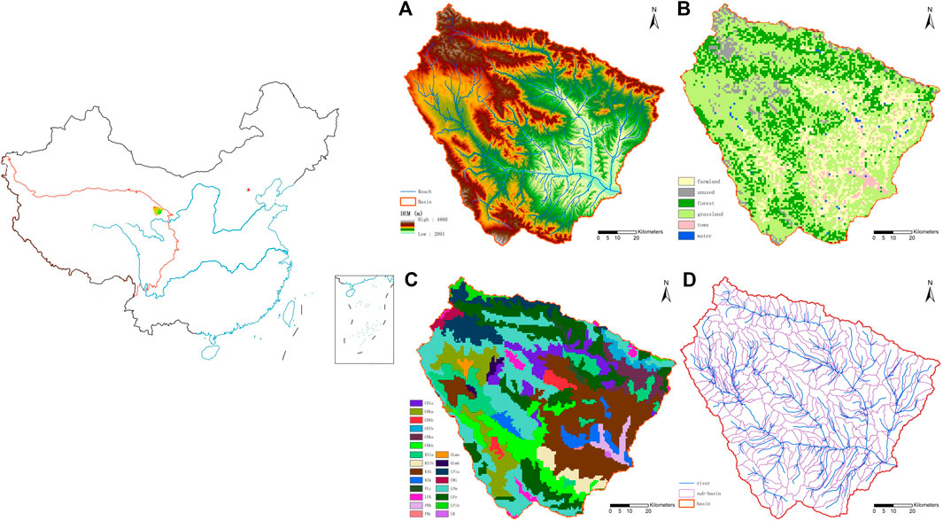
FIGURE 3. The graphic digital elevation model (DEM) data (A), land use data (B), soil data (C), and the divided threshold of the basin (D).

In this study, the mainstream Huangshui River and its tributaries were simulated. The hydrological data are from eight hydrological stations in the basin, including Huangyuan station (H1), Xining station (H2), Dongjiazhuang station (H3), Xinachuan station (H4), Niuchang station (H5), Qiaotou station (H6), Chaoyang Station (H7), and Fujiazhai station (H8). The daily flow monitoring data from 2008 to 2015 were used as the hydrological data in this study. Table 1 shows the results of the annual average flow of each hydrological station. Xining Station is located in the lower reaches of the Huangshui watershed, close to the exit of the basin, with an annual average flow of 39.99 m³/s. As the second largest hydrological station, Chaoyang station is located in the upper reaches of the confluence point of the Beichuan River, the main tributary of the Huangshui River basin, with an annual average flow of 20.58 m³/s. According to the statistics on the multiyear hydrologic flow data, the hydrologic situations had markable changes in different years. For example, the annual average flow of the Xining station in 2008 was 29.55 m³/s, which was only 57.7% of the annual average flow of 51.20 m³/s in 2014.

TABLE 1

TABLE 1. Annual average flow of each hydrological station.

The consistency of the time scales of the data utilized for the SDSM model, the GRNN model, and the SWAT model needs to be considered. The calibration periods, validation periods, and predictive periods were 1979–2000, 2001–2005, and 2021–2035, respectively, in the meteorological prediction section. In the hydrological simulation part, according to the daily hydrological data of the Huangshui watershed from 2008 to 2015, the relevant data from 2008 to 2013 were taken as the model training period, those of 2014–2015 were taken as the model validation period, and those of 2021–2035 were taken as the prediction period. In addition, the warm up period of the model was 3 years before the beginning time of the cycle.

4 Results Analysis and Discussion

4.1 The Prediction of the Meteorological Data

4.1.1 The temperature predictions by the Statistical Downscaling Method Model

The statistical parameter R² was used on the observation data and large-scale forecast of the daily maximum and minimum temperature from 1979 to 2000, and the R² values were approximately 0.9, which suggested that the temperature had a direct relation with the large-scale forecast factors and could be predicted directly. Moreover, the unconditional process analysis model of SDSM was applied to predict the monthly maximum and minimum average temperatures from 2021 to 2035.

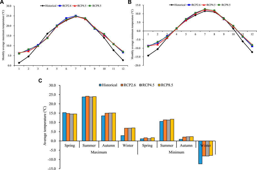
The predicted (each year from 2021 to 2035) and observed (each year from 1958 to 2011) maximum temperatures and the average minimum temperatures in different months are presented in Figure 4 and Table 2. Compared with the observed temperatures, the predicted maximum average temperatures of January, February, June, October, November, and December have an increasing tendency, and those of April, August, and September have an opposite tendency. However, the minimum average temperatures have an obvious increase in winter (November to February) and decrease slightly in summer (June to August). The prediction results suggested that considering the factors of climate change, the temperature fluctuation of the Huangshui watershed would become flatter, meaning that the temperature in winter would increase obviously, and the temperature difference within 1 year would decrease. The determination coefficients (R-squared) of the minimum temperature and maximum temperature were 0.77 and 0.62, respectively, and the Nash–Sutcliffe coefficients were 0.74 and 0.62. According to different season, the biggest change occurred in winter. The prediction maximum average temperatures will change from 2.87° to 7°, and the minimum average temperatures will change from −12.35° to −8°.

FIGURE 4

FIGURE 4. The predicted results of the monthly average temperatures.

TABLE 2

TABLE 2. The results of daily maximum temperature and minimum temperature in different periods.

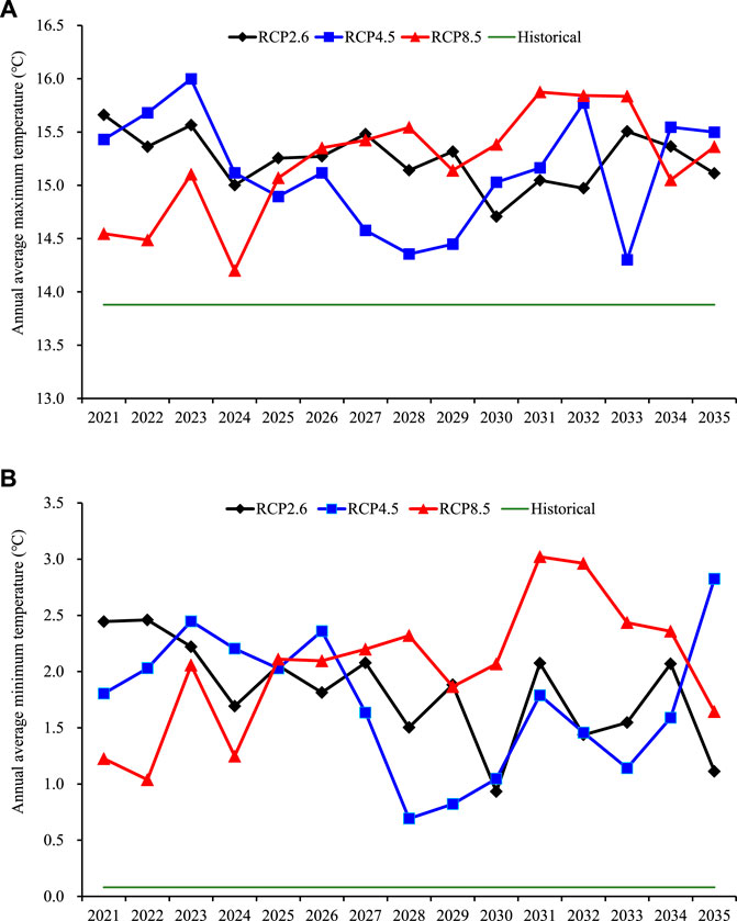
The annual average maximum temperatures and minimum temperatures of Xining station in the Huangshui watershed under different scenarios are shown in Figure 5. Under different scenarios, the average maximum temperatures and minimum temperatures at Xining station increased. The maximum temperature rose from 13.88° to 15.25°, 15.13°, and 15.21° in different scenarios. The minimum temperature rose from 0.08° to 1.82°, 1.72°, and 2.04°. Under the RCP8.5 scenario, the annual average maximum temperature showed an upward trend. However, in the RCP2.6 and RCP4.5 scenarios, the annual maximum temperatures showed certain downward trends. At the same time, the annual average minimum temperature showed an upward trend under the RCP85 scenario. Under the RCP2.6 and RCP4.5 scenarios, the annual average minimum temperatures presented certain downward trends. Overall, the maximum temperature and the minimum temperature showed the same trends under different scenarios. According to the analysis of different scenarios, the RCP2.6 scenario had a smaller temperature variation and stable climate between different years.

FIGURE 5

FIGURE 5. The predicted results of the annual average temperatures.

4.1.2 Precipitation Prediction by the Improved Generalized Regression Neural Network Model

Considering that daily rainfall is affected by atmospheric circulation, temperature, humidity, cloud cover, and other factors, seven factors (tas., pr., ths., ps., clt., uas., and vas.,) were selected as large-scale meteorological factors to predict daily precipitation. The generalized regression neural network was constructed and trained by using the historical meteorological data from 1979 to 2000.

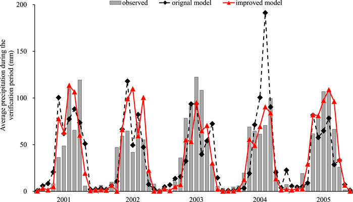
The daily precipitation in the verification period (2001–2005) is seen as the curve of the original net in Figure 6. The values of R² and NSE were 0.53 and 0.4, respectively, which were not sufficiently ideal. The forecast results of daily precipitation were also not ideal. This may be due to the strong randomness of daily precipitation on a daily time scale. To improve the predictive accuracy, the GRNN model was improved to construct a two-layer GRNN model in which the first layer took the monthly precipitation, monthly average near-surface air temperature, average near-surface wind, near-surface relative humidity, and surface air pressure as the inputs to predict the monthly precipitation. Then the monthly precipitation was induced into the second layer as the correction factor to predict the daily precipitation. The R² and NSE values obtained for the improved GRNN model were 0.72 and 0.70, respectively, suggesting that the accuracy of the results was improved and could reach a satisfactory level.

FIGURE 6

FIGURE 6. The simulated and observed monthly precipitations in the verification period (2001–2005).

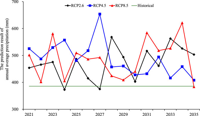
By combining the improved GRNN model with the large-scale meteorological data output by the CanESM2 model, the precipitation predictions of the Xining station under different RCPs were obtained. The annual average precipitation prediction results of the Xining station are shown in Figure 7. The annual average precipitation amounts of RCP2.6, RCP4.5, and RCP8.5 are 471.88, 486.98, and 485.67 mm, respectively, at Xining Station, which are very close. The annual average precipitation has an increasing tendency for RCP2.6 and RCP8.5, but a decreasing tendency for RCP4.5. Under the RCP2.6, RCP4.5, and RCP8.5 scenarios, the annual maximum precipitations are 568.06 mm at the year of 2028, 653.66 mm at the year of 2027, and 621.39 mm at the year 2034; the annual minimum precipitations are 372.00 mm at the year of 2024, 407.91 mm at the year 2035, and 383.45 mm at the year 2035.

FIGURE 7

FIGURE 7. The annual average precipitation prediction results of the Xining station.

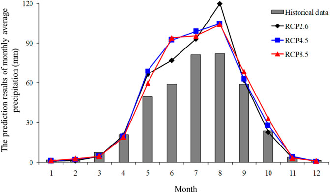
The monthly precipitation predictions and the observed precipitation data of Xining station are shown in Figure 8. It can be seen from the figure that during the dry season (November to April), the precipitation amounts of different RCPs have no obvious changes with the observed precipitation; however, for the precipitation of the wet season (May to September), the predicted precipitation has a large increase.

FIGURE 8

FIGURE 8. The monthly precipitation predictions and the observed precipitation data.

4.2 The Prediction of the Hydrologic Data

4.2.1 Calibration and Evaluation of the Parameters

The parameters used in this model were chosen as follows: First, the sensitivity ranking of the whole watershed parameters was conducted through the sensitivity analysis process, and the parameters ranked at the top were selected. At the same time, the parameters to be calibrated, their alternative methods, and initial rate determination range were determined in combination with the results of the SWAT manual and related research as well as the watershed related literature. Finally, 20 parameters and their initial value ranges were obtained. The original data in this paper were mainly used to calibrate the parameters and compare the simulation results with the final evaluation to determine the simulation effects of the model.

The daily flow rate data from 2008 to 2013 were set as the model calibration period, and those of 2014 and 2015 were set as the validation period of the model, and the 3 years before the calibration period were set as the model reheating period. The calibration was conducted for the eight hydrologic stations of the Huangshui watershed according to the principles of branches first and then main streams, up streams first and then down streams. The SWATCUP model was calibrated by the universal Sufi2 (Sequential Uncertainty Fitting Version 2) method, which takes the nondeterminacies of the input data, model structures, parameters, and metrical data into consideration and reflected the nondeterminacies to the ranges of the parameters. After the parameter calibration, the uncertainty interval at the 95% confidence level could contain most measured data.

The observed results of the calibration period, optimum simulation results, and 95% confidence interval are shown in Figure 9. It could be suggested that the SWAT model could simulate the monthly variation characteristics of the flow rates in the Huangshui watershed by the results of the calibration period. It was suggested that the single peak and multiple peaks in Figure 9 were attributed to the flow-rate peaks. When there was one main heavy precipitation in a month or the times of precipitation were concentrated, a single peak appeared; when the heavy precipitation happened more than once in a month or the times of precipitation were dispersive, multiple peaks appeared.

FIGURE 9

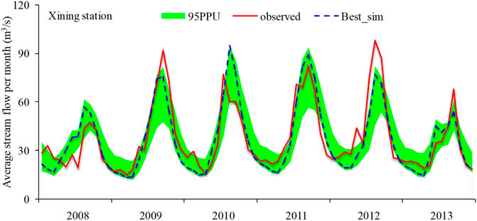
FIGURE 9. The observed results of the calibration period, optimum simulation results, and 95% confidence interval.

According to the variation characteristics of the observed and simulated results, it was concluded that the simulated results had smaller fluctuation ranges and that the value variation was more stable. In the wet seasons of the second (2009) and fifth years (2012) of the calibration period, the observed results were all higher than the optimum simulated results. The R² and NSE values of most hydrologic stations are approximately 0.75 and 0.70, respectively, which can properly reflect the whole flow rates of the Huangshui watershed.

The observed and updated simulated flow rate results in the verification period of the Xining hydrologic station are shown in Figure 10. The observed and simulated values are well fitted, especially for Xining Station, which is upstream of the basin main exit and can effectively reflect the variation characteristics of the flow rate with time.

FIGURE 10

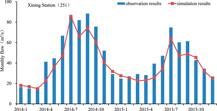
FIGURE 10. The observed and updated simulated flowrate results in the verification period of Xining station.

4.2.2 The Simulation and Prediction of the Hydrological Data

The parameters calibrated by the SWATCUP were input into the SWAT model to obtain runoff data at the exit of the Huangshui watershed from 2006 to 2015, which was set as the basic period. The average amount of runoff was 49.59 m³/s, and 2007 and 2013 had the largest and smallest runoff amount, at 60.83 and 37.31 m³/s, respectively. The runoff data were set as the basic data for the hydrological analysis under different climate change scenarios.

The predicted meteorological data at different RCPs were applied in the SWAT model with the calibrated parameters of the Huangshui Basin. The predicted runoff data at the exit of the basin under different RCPs are shown in Figure 11. It was suggested that under different RCPs, there was a large distinction among the runoff data, and the runoff data were 64.59, 59.20, and 49.61 m³/s for RCP2.6, RCP4.5, and RCP8.5, respectively. In addition, with the increase in CO₂ emission, the flow rate was larger than the flow rate between 2006 and 2015, which was 49.59 m³/s.

FIGURE 11

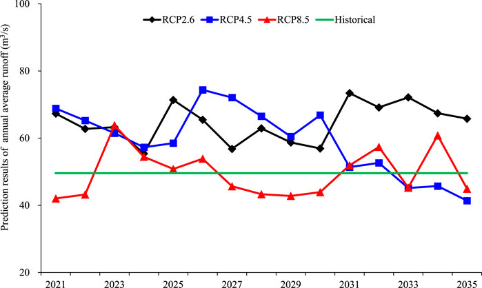
FIGURE 11. The predicted runoff data at the exit of the basin under different representative concentration pathways (RCPs).

4.3 Basin Water Availability Assessment

4.3.1 Analysis of Basin Ecological Water Demand

Based on monthly runoff, the original Tennant method divides the whole year into two periods and calculates the percentages of average annual flow. The first period is from October to March, and the second period is from April to September. Actually, the distinct regional characteristics and the monthly runoffs of the Huangshui watershed force the redivision of these two periods. According to the monthly average runoff data of the Xiaoxia Bridge section from 2006 to 2015, it is at the exit of the Huangshui River basin. It can be estimated that the annual average runoff of the Huangshui watershed is 49.59 m³/s. The average runoff from December to April is almost under 30 m³/s, which accounts for 22% of the annual overall runoff. Specifically, only runoff flow of 23.73 m³/s can be found in March. In comparison, the average runoff in each month from May to November is above 40 m³/s, which occupies 78% of the annual overall runoff. During the period from July to September, the average runoff can reach 80 m³/s. Thus, this study divides the whole year into two periods, from December to April and from May to November. Moreover, in consideration of the convenience of calculation, different levels of runoff percentage are recommended based on the runoff ratios at different time periods.

In this study, the Huangshui River is the largest tributary of the Yellow River, which contains high sediment due to the influence of geological conditions and human factors. The detention period of the sediment is from June to September. From the annual calculation of the mean annual sediment transport at Xining station, the mean annual sediment content in the Huangshui River is 2.45 kg/m³. Thus, it is necessary to attach the calculation of the sediment-carrying water volume on the original Tennant to ensure that the Huangshui River has enough water to transport the sediment in the water body downstream. Since sediment transport is mainly concentrated in the flood season, the sediment-carrying water volume of the Huangshui River during the flood season is 35 m³/t.

The average annual sediment-carrying water volume in the Huangshui watershed is approximately 134 million m³, accounting for 8.58% of the overall average annual runoff. The ecological water demand in the river channel accounts for 60.00% of the overall annual average runoff under the optimal conditions, and the proportion of the sediment-carrying water demand is 8.58%. Based on the results, the recommended final ecological base flow is 68.58% of the annual average runoff.

4.3.2 Basin Water Availability Assessment and Prediction

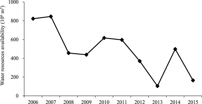
Since the total amount of basin water availability is equal to the difference between the basin average annual runoff and the ecological water demand, the basin hydrological simulation and the runoff under different climate scenarios can be predicted. Figure 12 illustrates the water availability from 2006 to 2015. It is worth noting that the optimal mean annual ecological water demand in the Huangshui River is 1.072 billion m³.

FIGURE 12

FIGURE 12. The average water availability in the Huangshui River in the baseline period.

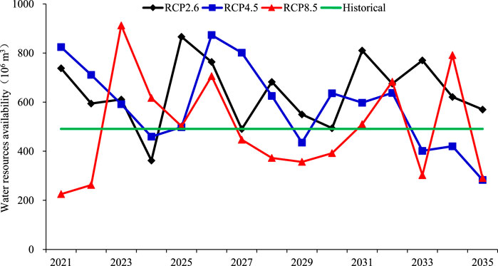
From 2006 to 2015, the mean annual average water availability in the Huangshui River was approximately 491 million m³. The largest water availability was 846 million m³ in 2007. The lowest value was 104 million m³ in 2013, which accounted for 12.29% of that in 2007. Taking the average annual runoff in different periods as input data, the ecological water demand in different planning periods under various scenarios can be calculated. The results of water availability in the Huangshui watershed are obtained during the forecast period under different concentration emission scenarios, as shown in Figure 13. In terms of the low-concentration emission scenario RCP2.6, the mean annual average water availability is 640 million m³. The largest water availability is predicted to reach almost 833 million m³ in 2025. In contrast, the lowest data point is predicted to be 362 million m³ in 2024. Different results can be obtained in the medium concentration emission scenario RCP4.5. The mean annual average water availability will decline to 587 million m³, accompanied by the largest data being 874 million m³ in 2026 and the least data being 492 million m³ in 2035. For the high concentration emission scenario RCP8.5, the water availability will witness a dramatic decrease, which falls to 492 million m³. Evidently, the range of the water availability in scenario RCP8.5 will be the largest among the three different emission scenarios, accompanied by a maximum of 913 million m³ in 2023 and a minimum of 225 million m³ in 2021.

FIGURE 13

FIGURE 13. The annual average water availability under different scenarios.

The results show that the Huangshui watershed is obviously affected by global climate change. With the increase in atmospheric CO₂ concentration and the further aggravation of greenhouse effects in the future, more obvious changes will be found in regional climate conditions. In the future, research and management in the Huangshui watershed need to fully consider the changes in temperature, precipitation, and other environmental factors. For example, when making a water resource allocation management plan, the decision-maker could make a flexible allocation plan in advance according to the change in trend of water resources available. Some emergency plans or engineering measures need to be developed in advance based on the predicted results. The results also indicate that climate change may have a positive effect on the ecological environment of the Qinghai–Tibet Plateau and other special regions. This means that rainfall in the region will increase as a result of climate change, and the temperature difference will decrease throughout the year. The region could shift from a semi-arid zone to a warm-humid zone, and ecosystems would benefit. The economic and social development of humanity in the region will also benefit from an increase in the availability of water resources.

In this study, the statistical downscaling method, the GRNN model, the SWAT model, and the improved Tennant method has been coupled. However, there are some shortcomings in this study, which need to be improved in several aspects. For example, in the further research, the researchers need to consider the response relationship between land use change and climate change. The hydrological change trend under the superposition of land use change and climate change should to be studied. The uncertainty in the research also needs to be considered, especially the problem of uncertainty amplification and superposition caused by the coupling of different methods. At the same time, the selection of large-scale meteorological data itself also needs repeated comparative analysis to select data sets with better applicability.

5 Conclusion

The Huangshui watershed is an ecologically fragile area on the Qinghai–Tibet Plateau of China. The meteorological and hydrological data of the Huangshui watershed were simulated under different climate change scenarios. In the simulation process, the temperature was predicted by the SDSM model; the precipitation data were simulated by the improved GRNN model; furthermore, the meteorological data were applied in the SWAT model to simulate the hydrologic processes at the basin scale under various climate change scenarios.

Through these simulations, it was determined that the basin temperatures were obviously changed by climate change, the improved GRNN model adopted in this study could effectively simulate the daily precipitation, and the R² and NSE values of the predicted results were significantly improved. Through the prediction results of the temperature and precipitation, the SWAT model could effectively simulate and predict the hydrological changes in the basin under the influence of climate change.

Moreover, the improved Tennant method is tailor-made for the variety of hydrological characteristics and the high sediment content in the river basin. The conclusion can be drawn that climate change has a great impact on water availability. The downscaling methods combined with the SWAT model and the calculation method of water availability have been proven effective in the study area. It was predicted that the temperature of the studied region would become flatter on the existing basis. Also, the precipitation would have a great increase in the wet season from May to September. In addition, the runoff of the Huangshui watershed and the water resource availability would decrease with increasing carbon emissions under different representative concentration pathway (RCP) scenarios. Moreover, the study could also provide an effective method to assess the regional hydrology and climate systems affected by climate change in ecotones similar to the Huangshui watershed.

Data Availability Statement

The raw data supporting the conclusion of this article will be made available by the authors, without undue reservation.

Author Contributions

ZF, YX, and HG designed the research. ZF wrote the original draft of this manuscript. YZ and XJ performed the analysis of the data and results. YX and SW revised the manuscript. All authors contributed to the article and approved the submitted version.

Funding

This research was funded by the Central Public-Interest Scientific Institution Basal Research Fund of Chinese Research Academy of Environmental Science (2020YSKY-014), the National Key Research and Development Program of China (2016YFA0601502), the Program for Guangdong Introducing Innovative and Entrepreneurial Teams (2019ZT08L213), Beijing Natural Science Foundation (No. 9212001), and the National Natural Science Foundation of China (51609003).

Conflict of Interest

The authors declare that the research was conducted in the absence of any commercial or financial relationships that could be construed as a potential conflict of interest.

Publisher’s Note

All claims expressed in this article are solely those of the authors and do not necessarily represent those of their affiliated organizations, or those of the publisher, the editors and the reviewers. Any product that may be evaluated in this article, or claim that may be made by its manufacturer, is not guaranteed or endorsed by the publisher.

Supplementary Material

The Supplementary Material for this article can be found online at: https://www.frontiersin.org/articles/10.3389/feart.2021.755119/full#supplementary-material

References

Abbaspour, K. C., Yang, J., Maximov, I., Siber, R., Bogner, K., Mieleitner, J., et al. (2007). Modelling Hydrology and Water Quality in the pre-alpine/alpine Thur Watershed Using SWAT. J. Hydrol. 333, 413–430. doi:10.1016/j.jhydrol.2006.09.014

CrossRef Full Text | Google Scholar

Arnold, J. G., Daniel, N. M., Philip, W. G., Karim, C. A., and Manoj, K. J. (2012). SWAT: Model Use, Calibration, and Validation [J]. Trans. Asabe 55, 1549–1559. doi:10.13031/2013.42256

CrossRef Full Text | Google Scholar

Ateeq-Ur, R., and Abdul, G. (2018). Impact Assessment of Rainfall-Runoff Simulations on the Flow Duration Curve of the Upper Indus River-A Comparison of Data-Driven and Hydrologic Models [J]. Water 10 (7), 876. doi:10.3390/w10101411

CrossRef Full Text | Google Scholar

Chen, D. L., Xu, B. Q., Yao, T. D., Guo, Z. T., Cui, P., Chen, F. H., et al. (2015). Assessment of Past, Present and Future Environmental Changes on the Tibetan Plateau [J]. Chin. Sci. Bull., 3025–3035. doi:10.1360/n972014-01370

CrossRef Full Text | Google Scholar

Cigizoglu, H. K., and Alp, M. (2006). Generalized Regression Neural Network in Modelling River Sediment Yield. Adv. Eng. Softw. 37 (2), 63–68. doi:10.1016/j.advengsoft.2005.05.002

CrossRef Full Text | Google Scholar

Dalkilic, Y., Okkan, U., and Baykan, N. (2014). Comparison of Different Ann Approaches in Daily Pan Evaporation Prediction[J]. J. Water Resource Prot. 6 (4), 319–326. doi:10.4236/jwarp.2014.64034

CrossRef Full Text | Google Scholar

Delworth, T. L. (2006). GFDL's CM2 Global Coupled Climate Models. Part I: Formulation and Simulation Characteristics [J]. J. Clim. 19 (19), 643–674. doi:10.1175/jcli9016.1

CrossRef Full Text | Google Scholar

Friedlingstein, P., Meinshausen, M., Arora, V. K., Jones, C. D., Anav, A., Liddicoat, S. K., et al. (2014). Uncertainties in CMIP5 Climate Projections Due to Carbon Cycle Feedbacks. J. Clim. 27 (2), 511–526. doi:10.1175/jcli-d-12-00579.1

CrossRef Full Text | Google Scholar

Ghosh, S., and Mujumdar, P. P. (2008). Statistical Downscaling of GCM Simulations to Streamflow Using Relevance Vector Machine. Adv. Water Resour. 31 (1), 132–146. doi:10.1016/j.advwatres.2007.07.005

CrossRef Full Text | Google Scholar

Guo, Y., Li, J., and Li, Y. (2014). Seasonal Forecasting of North China Summer Rainfall Using a Statistical Downscaling Model. J. Appl. Meteorology Climatology 53 (7), 1739–1749. doi:10.1175/jamc-d-13-0207.1

CrossRef Full Text | Google Scholar

Hanewinkel, M., Cullmann, D. A., Schelhaas, M.-J., Nabuurs, G.-J., and Zimmermann, N. E. (2013). Climate Change May Cause Severe Loss in the Economic Value of European forest Land. Nat. Clim Change 3 (3), 203–207. doi:10.1038/nclimate1687

CrossRef Full Text | Google Scholar

Hughes, D. A., and Mazibuko, S. (2018). Simulating Saturation-Excess Surface Run-Off in a Semi-distributed Hydrological Model. Hydrological Process. 32 (17), 2685–2694. doi:10.1002/hyp.13182

CrossRef Full Text | Google Scholar

Jeong, D. I., St-Hilaire, A., Ouarda, T. B. M. J., and Gachon, P. (2012). Multisite Statistical Downscaling Model for Daily Precipitation Combined by Multivariate Multiple Linear Regression and Stochastic Weather Generator [J]. Climatic Change 114 (3-4), 567–591. doi:10.1007/s10584-012-0451-3

CrossRef Full Text | Google Scholar

Joseph, N., Preetha, P. P., and Narasimhan, B. (2021). Assessment of Environmental Flow Requirements Using a Coupled Surface Water-Groundwater Model and a Flow Health Tool: A Case Study of Son River in the Ganga basin. Ecol. Indicators 121, 107110. doi:10.1016/j.ecolind.2020.107110

CrossRef Full Text | Google Scholar

Kattsov, V. M., Walsh, J. E., Chapman, W. L., Govorkova, V. A., Pavlova, T. V., and Zhang, X. (2007). Simulation and Projection of Arctic Freshwater Budget Components by the IPCC AR4 Global Climate Models. 2007 8 (3), 571–589. doi:10.1175/jhm575.1

CrossRef Full Text | Google Scholar

Kumar, G., and Malik, H. (2016). Generalized Regression Neural Network Based Wind Speed Prediction Model for Western Region of India [J]. Proced. Comp. Sci. 93, 26–32. doi:10.1016/j.procs.2016.07.177

CrossRef Full Text | Google Scholar

Meenu, R., Rehana, S., and Mujumdar, P. P. (2013). Assessment of Hydrologic Impacts of Climate Change in Tunga-Bhadra River basin, India with HEC-HMS and SDSM. Hydrol. Process. 27 (11), 1572–1589. doi:10.1002/hyp.9220

CrossRef Full Text | Google Scholar

Nyikadzino, B., Chitakira, M., Muchuru, S., and Muchuru, S. (2020). Rainfall and Runoff Trend Analysis in the Limpopo River basin Using the Mann Kendall Statistic. Phys. Chem. Earth, Parts A/B/C 117, 102870. doi:10.1016/j.pce.2020.102870

CrossRef Full Text | Google Scholar

Park, C.-E., Jeong, S.-J., Joshi, M., Osborn, T. J., Ho, C.-H., Piao, S., et al. (2018). Keeping Global Warming within 1.5 °C Constrains Emergence of Aridification. Nat. Clim Change 8 (1), 70–74. doi:10.1038/s41558-017-0034-4

CrossRef Full Text | Google Scholar

Piras, M., Mascaro, G., Deidda, R., and Vivoni, E. R. (2015). Impacts of Climate Change on Precipitation and Discharge Extremes through the Use of Statistical Downscaling Approaches in a Mediterranean basin. Sci. Total Environ. 543, 952–964. doi:10.1016/j.scitotenv.2015.06.088

PubMed Abstract | CrossRef Full Text | Google Scholar

Sharma, A., and Goyal, M. K. (2020). Assessment of the Changes in Precipitation and Temperature in Teesta River basin in Indian Himalayan Region under Climate Change. Atmos. Res. 231, 104670. doi:10.1016/j.atmosres.2019.104670

CrossRef Full Text | Google Scholar

Sillmann, J., Kharin, V. V., Zwiers, F. W., Zhang, X., and Bronaugh, D. (2013). Climate Extremes Indices in the CMIP5 Multimodel Ensemble: Part 2. Future Climate Projections. J. Geophys. Res. Atmos. 118 (6), 2473–2493. doi:10.1002/jgrd.50188

CrossRef Full Text | Google Scholar

Song, X., Yang, G., Yan, C., Duan, H., Liu, G., and Zhu, Y. (2009). Driving Forces behind Land Use and Cover Change in the Qinghai-Tibetan Plateau: a Case Study of the Source Region of the Yellow River, Qinghai Province, China. Environ. Earth Sci. 59 (4), 793–801. doi:10.1007/s12665-009-0075-8

CrossRef Full Text | Google Scholar

Song, Y., Linderholm, H. W., Wang, C., Tian, J., Huo, Z., Gao, P., et al. (2019). The Influence of Excess Precipitation on winter Wheat under Climate Change in China from 1961 to 2017. Sci. Total Environ. 690, 189–196. doi:10.1016/j.scitotenv.2019.06.367

PubMed Abstract | CrossRef Full Text | Google Scholar

Specht, D. F. (1991). A General Regression Neural Network. IEEE Trans. Neural Netw. 2, 568–576. doi:10.1109/72.97934

PubMed Abstract | CrossRef Full Text | Google Scholar

Suwal, N., Kuriqi, A., Huang, X. F., Delgado, J., Młyński, Da., and Walega, A. (2020). Environmental Flows Assessment in Nepal: The Case of Kaligandaki River [J]. Sustainability 12 (21), 1–23. doi:10.3390/su12218766

CrossRef Full Text | Google Scholar

Tang, J., Niu, X., Wang, S., Gao, H., Wang, X., and Wu, J. (2016). Statistical Downscaling and Dynamical Downscaling of Regional Climate in China: Present Climate Evaluations and Future Climate Projections. J. Geophys. Res. Atmos. 121 (5), 2110–2129. doi:10.1002/2015jd023977

CrossRef Full Text | Google Scholar

Taylor, K. E., Stouffer, R. J., and Meehl, G. A. (2012). An Overview of CMIP5 and the Experiment Design. Bull. Am. Meteorol. Soc. 93 (4), 485–498. doi:10.1175/bams-d-11-00094.1

CrossRef Full Text | Google Scholar

Teng, M., Zeng, L., Hu, W., Wang, P., Yan, Z., He, W., et al. (2020). The Impacts of Climate Changes and Human Activities on Net Primary Productivity Vary across an Ecotone Zone in Northwest China. Sci. Total Environ. 714, 136691. doi:10.1016/j.scitotenv.2020.136691

PubMed Abstract | CrossRef Full Text | Google Scholar

Thuiller, W., Lavorel, S., Araujo, M. B., Sykes, M. T., and Prentice, I. C. (2005). Climate Change Threats to Plant Diversity in Europe. Proc. Natl. Acad. Sci. 102 (23), 8245–8250. doi:10.1073/pnas.0409902102

PubMed Abstract | CrossRef Full Text | Google Scholar

Whitehead, P. G., Wilby, R. L., Battarbee, R. W., Kernan, M., and Wade, A. J. (2009). A Review of the Potential Impacts of Climate Change on Surface Water Quality. Hydrological Sci. J. 54 (1), 101–123. doi:10.1623/hysj.54.1.101

CrossRef Full Text | Google Scholar

Wilby, R. L., Dawson, C. W., and Barrow, E. M. (2002). Sdsm - a Decision Support Tool for the Assessment of Regional Climate Change Impacts. Environ. Model. Softw. 17 (2), 145–157. doi:10.1016/s1364-8152(01)00060-3

CrossRef Full Text | Google Scholar

Yakup, K., Aydın, H. D., and Zehra, Y. (2018). Comparison of Environmental Flow Assessment Methods with a Case Study on a Runoff River–type Hydropower Plant Using Hydrological Methods [J]. Environ. Monit. Assess. 190 (12), 1–15. doi:10.1007/s10661-018-7107-3

CrossRef Full Text | Google Scholar

Zhang, L., Zhao, Y., Hein-Griggs, D., Janes, T., Tucker, S., and Ciborowski, J. J. H. (2020). Climate Change Projections of Temperature and Precipitation for the great lakes basin Using the PRECIS Regional Climate Model. J. Great Lakes Res. 46 (2), 255–266. doi:10.1016/j.jglr.2020.01.013

CrossRef Full Text | Google Scholar