A High-Resolution Gravimetric Geoid Model for Kuwait Using the Least-Squares Collocation

A new gravimetric geoid model, the KW-FLGM2021, is developed for Kuwait in this study. This new geoid model is driven by a combination of the XGM2019e-combined global geopotential model (GGM), terrestrial gravity, and the SRTM 3 global digital elevation model with a spatial resolution of three arc seconds. The KW-FLGM2021 has been computed by using the technique of Least Squares Collocation (LSC) with Remove-Compute-Restore (RCR) procedure. To evaluate the external accuracy of the KW-FLGM2021 gravimetric geoid model, GPS/leveling data were used. As a result of this evaluation, the residual of geoid heights obtained from the KW-FLGM2021 geoid model is 2.2 cm. The KW-FLGM2021 is possible to be recommended as the first accurate geoid model for Kuwait.

Introduction

The geoid is an important surface to use in geomatics, geophysics, geodesy, and several Earth sciences. In geodesy, it plays an important role as a fundamental datum of the heights (Sansò and Sideris, 2013). As a result of the widespread and fast usage of the Global Navigation Satellite Systems (GNSSs), they have been revolutionized in the fields of geomatics and navigation, and replaced the classical methods of mapping. In particular, GNSS offers accurate geodetic measurements in significantly less time. GNSS is a 3-D system that provides ellipsoidal heights relative to the ellipsoid surface. Unfortunately, ellipsoidal heights are just a geometrical quantity, and its conversion to orthometric height using the geoid model is widely used in almost all day-to-day applications requiring height information (Torge and Müller, 2012; Sansò and Sideris, 2013).

The geoid heights can be obtained by subtracting the ellipsoidal and orthometric heights. In turn, the ellipsoidal and geoidal heights may be used to estimate the orthometric height. A high-resolution geoid should be determined to be able to deal with GNSS height accuracy levels that allow the orthometric height to be derived by integrating Geoid and GNSS (Hofmann-Wellenhof and Moritz, 2006). The computation of regional gravimetric geoids has increased in recent years (Huang and Véronneau, 2013; Zaki, 2015; Zaki, 2018; Matsuo and Kuroishi, 2020; Saadon et al., 2021; Varga et al., 2021; Zaki and Mogren, 2021). Geoid determination theory and methods have been improved (Moritz, 1978; Forsberg and Sideris, 1993; Sjöberg, 2003; Ellmann and Vaníček, 2007; Shen and Han, 2013); the availability of accurate and high-resolution digital elevation and digital bathymetry models (Hennig et al., 2001; Olson et al., 2014), the computation of accurate global geopotential models (Pavlis, 2008; Förste et al., 2015; Zingerle et al., 2020), the prospect of fitting the gravimetric geoid model with the GNSS/leveling and using diverse data efficiently are the major factors that made the computation of accurate geoid model possible (Erol, 2007; Kaloop et al., 2018; Kaloop et al., 2020; Kaloop et al., 2021).

For Kuwait state, there are no previous studies to calculate the gravimetric geoid. So, the major goal of this research is to develop a high-resolution geoid for Kuwait, which will enable the country to obtain accurate orthometric heights from GNSS observation instead of the time and effort-consuming slow-spirit leveling process.

Data

Terrestrial Gravity Data

Kuwait has constructed a national gravity network consisting of 93 stations spaced 10–15 km apart. Figure 1 shows the distribution of these points. The values of the free air anomalies (FA) range between −36.93 mGal and 2.04 mGal with an average and a standard deviation (STD) of −17.03 and 8.69 mGal, respectively. The full details about the terrestrial gravity data are described in El-Ashquer et al., (2020). The accuracy of observed gravity is about 0.22 mGa l on STD, according to comparisons with different surveying campaigns (El-Ashquer et al., 2020).

FIGURE 1

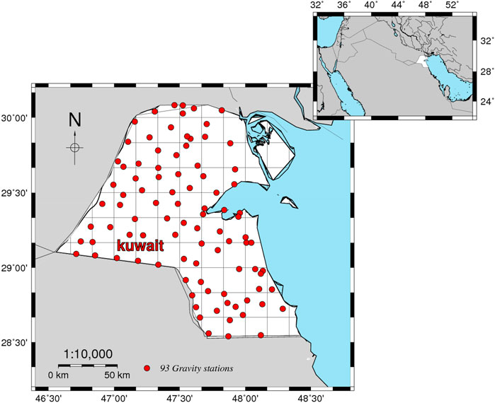
FIGURE 1. The terrestrial gravity data distribution in Kuwait.

GPS/Leveling Stations

In this study, 83 GPS/leveling stations are used. The distribution of these GPS/leveling stations is shown in Figure 2. The benchmark GPS coordinates were determined using the static and rapid-static measurement methods and the ITRF2008 datum using dual-frequency GPS devices. The horizontal and vertical accuracy are around 1 and 1.5 cm, respectively (El-Ashquer et al., 2020).

FIGURE 2

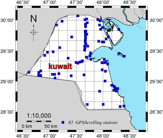
FIGURE 2. The GPS/leveling points in Kuwait.

Through the use of high-precision spirit leveling, the orthometric heights of the 83 stations were connected to the vertical datum of the Kuwait Public Work Department (Kuwait PWD). The accuracy of the orthometric heights is approximately 1.0 cm. The GPS/leveling-based geoid heights range between −18.54 and −10.95 m with an average value of −15.45 m and an STD of 1.51 m. More details about the GPS/leveling station are described in El-Ashquer et al., (2020).

Digital Elevation Model

Kuwait has a smooth topography and a slightly uneven desert. The slopes of lands are gradually from the Arabian Gulf in the east to the southwest and west. The southwestern corner heights reach 300 m above sea level. In Kuwait, there are small hills spread all over the country.

The digital elevation model (DEM) reflects the topographic features of the Earth in a digital format. A significant gravitational signal is produced by the topographic masses, and this signal dominates the gravitational spectrum in shorter wavelengths. Before any modeling method, the gravitational field can be smoothed by removing the contribution of topography. Approximately 2 and 34% of the signals of geoid heights and gravity anomaly components are present in short wavelengths, that is, high frequencies from harmonic degrees 360 to 36,000, so that the topographic effects play a significant role (Schwarz, 1984).

The accuracy of the DEM is of paramount importance in geoidal computation because the errors in the DEM are propagated in geoidal models during the calculation of the free-air gravity anomalies, as well as afterward in the computation of the topographical effect. In the current study, over areas of land, SRTM3arc v4.1 with a resolution of around 90 m (Hennig et al., 2001) was used. Over marine areas, the bathymetric model with a 15″ resolution was used from SRTM15arc plus (Olson et al., 2014). SRTM15arc plus was griding to 3″ in the Arabian Gulf and combined with the SRTM3 (Figure 3). The created DEM has been evaluated by using the orthometric heights in the GPS/leveling stations. As a result of these comparisons, the differences had a minimum, maximum, mean, and STD of −3.41, 13.84, 2.38, and 2.56 m, respectively.

FIGURE 3

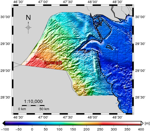
FIGURE 3. The 3″ × 3″ DEM for Kuwait.

Global Geopotential Model

In this research, the XGM2019e GGM (Zingerle et al., 2020) up to degree 2,190 is used. XGM2019e is a combined global geopotential model up to degree and order (d/o) 5,540, corresponding to a resolution of 2′ (∼4 km). The sources of data in XGM2019e include the GOCO06s (Kvas et al., 2019) up to d/o 300 and ground gravity anomalies from the US National Geospatial-Intelligence Agency (NGA), with resolution 15′, identical to XGM2016 (Pail et al., 2018) and enhanced with topographic gravity information from EARTH2014 (Rexer et al., 2017). In the offshore, gravity data are derived from the DTU13 satellite altimetric model (Andersen et al., 2013) with 1′ spatial resolution. Up to d/o 719 (15′), the gravity solution is performed by the combination between satellite and ground gravity grid from the NGA. Beyond d/o 719, the gravity solution is determined from EARTH2014 and DTU13.

In Zingerle et al. (2020), XGM2019e shows a slightly enhanced behavior in the comparison with other models such as EIGEN6c4 (Förste et al., 2015) and EGM2008 (Pavlis, 2008) in the spectral assessment for the band up to d/o 719. Global validation of the GNSS/leveling data indicates that the XGM2019e can be considered more reliable and consistent with existing high-degree global geopotential models (Zingerle et al., 2020).

Methodology and Theoretical Background

The computation of the new geoid model for Kuwait is based on the Remove-Compute-Restore technique (RCR) (Torge and Müller, 2012). The RCR technique decomposed the gravity signals into three parts: long, medium, and short wavelength. The long-wavelength components are obtained from the GGM, and the medium wavelength is derived from gravity information captured from terrestrial, shipborne, and airborne, as well as some satellite gravity missions. The components of the short wavelength are mostly the products from the topography of the Earth, which are usually derived from DEM (Hofmann-Wellenhof and Moritz, 2006).

The “remove” step for geoid determination in the RCR includes the elimination of the GGM and topographic contribution from the observed anomalies as Eq. 1 (Hofmann-Wellenhof and Moritz, 2006):

$\Delta g_{res}=\Delta g_{FA}-\Delta g_{GGM}-\Delta g_{RTM}(1)$

where $\Delta g_{res}$ is the residual gravity anomaly; $\Delta g_{FA}$ is the free-air gravity anomaly; $\Delta g_{GGM}$ is the gravity anomaly which represents the long-wavelength component from the GGM as Eq. 2, and $\Delta g_{RTM}$ is the topography-reduced gravity anomaly. In this study the topographic effect computation method is based on the residual terrain model (RTM) as Eq. 3 (Forsberg, 1984).

$\Delta g_{GGM}=\frac{GM}{r^2}{\displaystyle \sum }_{n=2}^{\infty }\left(n-1\right){\left(\frac{a}{r}\right)}^n{\displaystyle \sum }_{m=0}^n\left({\overline{C}}_{nm}\mathit{cos}m\lambda +{\overline{S}}_{nm}\mathit{sin}m\lambda \right){\overline{P}}_{nm}\left(\mathit{cos}\theta \right)(2)$

where GM denotes the geocentric gravitation constant, $a$ is the ellipsoid semi-major, $\lambda$ is the geodetic longitude, $r$ is the geocentric radius, n is the degree, m is the order, ${\overline{C}}_{nm}$ and ${\overline{S}}_{nm}$ are the fully normalized potential cosine and sine coefficients, ${\overline{P}}_{nm}$ denotes the fully normalized associated Legendre functions, ${\overline{P}}_{nm}$ denotes the fully normalized associated Legendre functions, and $\theta$ is the angular polar distance.

In the planar approximation, the RTM gravitational effect can be computed as the formula stated in Forsberg, (1984):

$\Delta g_{RTM} =2\pi G\rho \left(h_P-h_{ref}\right)-G{\displaystyle \underset{E}{\mathit{\iint }}{\displaystyle \underset{h_{ref}}{\overset{H}{\mathit{\int }}}\frac{\rho \left(x,y,z\right)\left(h_P-z\right)}{{\left[{\left(x_P-x\right)}^2+{\left(y_P-y\right)}^2+{\left(h_P-z\right)}^2\right]}^{\frac{3}{2}}}}}dxdydz(3)$

where $G$ is known as the gravitational constant, $h_{ref}$ represents the height of the smoothed DEM, $E$ is the planar projection, $h$ is the height of the DEM,$\rho \left(x,y,z\right)$ is the mean density of the Earth crust, that is, 2.67 $gm\Delta c{m}^{-3}$, $x,y,$ and $z$ are the Cartesian coordinates, and $x_P,y_P,$ and $h_P$ are the computational point’s coordinates and height on which the RTM is evaluated.

The “compute” step is computing the residual height anomaly $\left({\xi }_{res}\right)$ from the residual gravity anomaly $\left(\Delta g_{res}\right)$ with the least-squares collocation (LSC) method (Moritz, 1978) by applying the formula which can be written as follows:

${\text{ζ}}_{res}=C_{{\text{ζ}}_{res}\mathrm{\Delta }{\text{g}}_{res}}{C}_{\Delta {\text{g}}_{res}\Delta {\text{g}}_{res}}^{-1}\Delta {\text{g}}_{res}(4)$

where $C_{{\text{ζ}}_{res}\Delta {\text{g}}_{res}.}$ is the matrix of residual height anomalies’ cross-covariance and the residual gravity anomalies $\left[\left(\Delta {\text{g}}_{res}\right), C_{\Delta {\text{g}}_{res}\Delta {\text{g}}_{res}}\right]$ is the residual gravity anomalies’ empirical auto-covariance matrix.

The empirical auto-covariance function can be written as:

$co{v}_{\Delta {\text{g}}_{res}\Delta {\text{g}}_{res}}\left({\psi }_{ik}\right)=\frac{1}{N_{ik}}{{\displaystyle \sum }}_{i,k}^{N_{ik}}\Delta {\text{g}}_{res}\left({\phi }_i,{\lambda }_i\right)\Delta {\text{g}}_{res}\left({\phi }_k,{\lambda }_k\right)(5)$

where $N_{ik}$ is the number of the pairs for each interval and ${\psi }_{ik}$ is the spherical distance between pairs. So, ${\text{Δg}}_{\text{res}}$ has been considered in order to calculate the isotropic empirical covariance function by the EMPCOV subroutine of the GRAVSOFT (Forsberg and Tscherning, 2008). In the empirical estimation process of the isotropic covariance function, the spherical distance ${\psi }_{ik}$ is chosen with the condition that:

${\psi }_{ik}-\left(\text{Δ}\psi /2\right)<{\psi }_{ik}<{\psi }_{ik}+(\text{Δ}\psi /2)$Equation 6

The agreement between the empirical and analytical covariance functions illustrated the statistical homogeneity of the residual gravity anomaly distribution used in this study. The latter covariance function is required to carry out the calculations using the LSC technique, in which the required auto and cross-covariance functions are obtained from the analytically modeled local covariance function, which is stated as follows (Tscherning, 2013):

$cov(T\left(I\right),T\left(K\right)=\alpha {\displaystyle \sum }_{n=2}^{N_{max}}{\sigma }_n^2{\left(\frac{R_E^2}{r_I{r}_K}\right)}^{n+1}{P}_n\left(\cos {\psi }_{ik}\right)+{\displaystyle \sum }_{n=N_{max}+1}^{\infty }\left(\frac{A}{\left(n-1\right)\left(n-2\right)\left(n-4\right)}\right){\left(\frac{R_B^2}{r_I{r}_K}\right)}^{n+1}{P}_n(\cos {\psi }_{ik})(7)$

where T is the anomalous gravity potential (obtained from the error degree variances of the applied GGM, which in our case is XGM2019) at two points $I$ and $K$, which are separated by a spherical distance ${\psi }_{ik}$ and $r_I$, $r_K$ are the distances of the two points from the geo-center, $R_E$ is the mean Earth’s radius, $R_B$ is the radius of Bjerhammar sphere, ${\sigma }_n^2$ is the error degree variance, and $P_n\left(\cos {\psi }_{ik}\right)$ denotes the Legendre polynomial of degree n. The covariance parameters $\alpha$ (scale parameter), $A$ (a constant parameter in units of (m/s ${)}^4$), and $R_B$ are calculated using an iterative non-linear adjustment based on the $\Delta {\text{g}}_{res}$ and its empirical covariance function, which is utilized as input for the collocation process (Knudsen, 1987).

The height anomaly is restored in the ‘restore’ phase of the geoid and is expressed as Eq. 8:

$\xi ={\xi }_{GGM}+{\xi }_{res}+{\xi }_{RTM}(8)$

where $\xi$ is the gravimetric quasi-geoid model and ${\xi }_{GGM}$ is the GGM-derived quasi-geoid height in Eq. 9 (Hofmann-Wellenhof and Moritz, 2006):

${\xi }_{GGM}=\frac{GM}{\gamma r}{\displaystyle \sum }_{n=2}^{\infty }{\left(\frac{a}{r}\right)}^n{\displaystyle \sum }_{m=0}^n\left({\overline{C}}_{nm}\mathit{cos}m\lambda +{\overline{S}}_{nm}\mathit{sin}m\lambda \right){\overline{P}}_{nm}\left(\mathit{cos}\theta \right)(9)$

where γ is the normal gravity.

${\xi }_{res}$ is the residual geoid height from Eq. 4, and ${\xi }_{RTM}$ is the effect due to the topographic reduction which can be computed as Eq. 10 (Forsberg, 1984; Sansò and Sideris, 2013):

${\xi }_{RTM}=\frac{G}{\gamma }{\displaystyle \underset{\text{E}}{\iint }{\displaystyle \underset{h_{ref}}{\overset{h}{\int }}\frac{\rho \left(x,y,z\right)}{{[{(x_P-x)}^2+{(y_P-y)}^2+{(h_P-z)}^2]}^{\frac{1}{2}}}}}\text{ dx dy dz }(10)$

The final step to compute the gravimetric geoid is the conversion of geoid height anomaly to geoid undulation, which can be done by adding a contribution from the Bouguer anomaly as (Moritz, 1978; Forsberg, 1984):

$N\approx \xi +\frac{\Delta g_B}{\overline{\gamma }}H(11)$

where N represents the geoid height, $\xi$ is the height anomaly, $\Delta g_B$ denotes the Bouguer gravity anomaly, $\overline{\gamma }$ is the mean normal gravity, and H is the orthometric height.

In the following sections, the numerical results to compute the gravimetric geoid are discussed in detail.

Result and Discussion

The Remove-Compute-Restore

The geoid model for Kuwait was calculated using the technique described in Section 3. Table 1 displays the estimated statistical values of the $\Delta {\text{g}}_{\text{FA}}$ and $\Delta {\text{g}}_{res}$. Removing the effects of the long wavelengths has been fulfilled by removing the effect of the reference GGM XGM2019e up to d/o 2,190, from the $\Delta {\text{g}}_{\text{FA}}$ data. The contribution of topography (${\text{Δg}}_{RTM})$ has been calculated with the TC program (Forsberg and Tscherning, 2008) using the RTM model, at a radius of 100 km of the running point (Forsberg, 1984). A constant density value has been accounted for the topography equivalent to $\rho =2.67{\text{ gcm}}^{-3}$.

TABLE 1

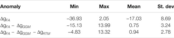
TABLE 1. Statistics of residual gravity anomalies (mGal).

Removing the component of the long-wavelength $\left(\text{Δ}{\mathrm{g}}_{\mathit{GGM}}\right)$ from the $\text{Δ}{\mathrm{g}}_{\mathit{FA}}$ results in significant smoothing, as seen by a decrease in standard deviations (STD) from 8.69 mGal to 3.24 mGal (about 62%). The smoothing is observed after removing the short-wavelength components of the gravity signal from the local topography, a slight refinement of the STD from 3.24 mGal to 2.78 mGal.

Several trials have been performed to estimate the best fitting between the empirical and analytical covariance functions for $\Delta g_{res}$ . By using different spherical distance $\text{Δ}\psi$, the EMPCOV program (Forsberg and Tscherning, 2008) is used to compute the values which make the best fitting with covariance model value in the COVFIT program (Forsberg and Tscherning, 2008). As shown in Figure 4, the fitting between empirical auto-covariance functions (red line) and covariance function model for the reduced values obtained with XGM2019 is plotted up to degree 2,190 (blue line) (Tscherning and Rapp, 1974) at $\text{Δ}\psi$. 10 arc-minutes is the best fitting value.

FIGURE 4

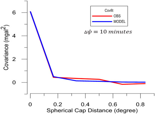
FIGURE 4. Fitted empirical and analytical covariance functions for the $\Delta g_{res}$ at a spherical distance of 10 arc minutes.

The best fit covariance model has the following parameters estimated by using the COVFIT program: (AA) is error degree variance scale factor of 0.0194, depth to the Bjerhammer sphere = −6.418 km, that is, ($R_E-R_B)$, and (VARG) is the variance of gravity anomalies at zero altitudes is 6.65 mGa ${\text{l}}^2$. The residual height anomalies were calculated using these estimated parameters on a 6′ × 6′ grid from $\Delta g_{res}$ by using the GEOCOL program (Forsberg and Tscherning, 2008).

The compute step in the RCR procedure was then followed by the restore step. Following that, the impact of both eliminated components, that is, the long (${\text{ζ}}_{GGM}$) coming from GGM XGM2019 at (d/o) 2,190 and topographic short-wavelength component (${\text{ζ}}_{RTM}$), was then restored and added to the ${\text{ζ}}_{res}$ at the computation points of prediction on a 6′ × 6′ mesh grid to compute the height anomaly ζ values as Eq. 8.

Figure 5 depicts the many estimated components used to recreate the gravimetric geoid/quasigeoid model. Figure 5A illustrates the residual height anomalies ${\text{ ζ}}_{res}$, whereas Figure 5B demonstrates that the estimated error of the calculations of ${\text{ζ}}_{res}$ ranges from 0.5 to 1.1 cm, with mean values of roughly 1.01 cm and a standard deviation of 0.14 cm.

FIGURE 5

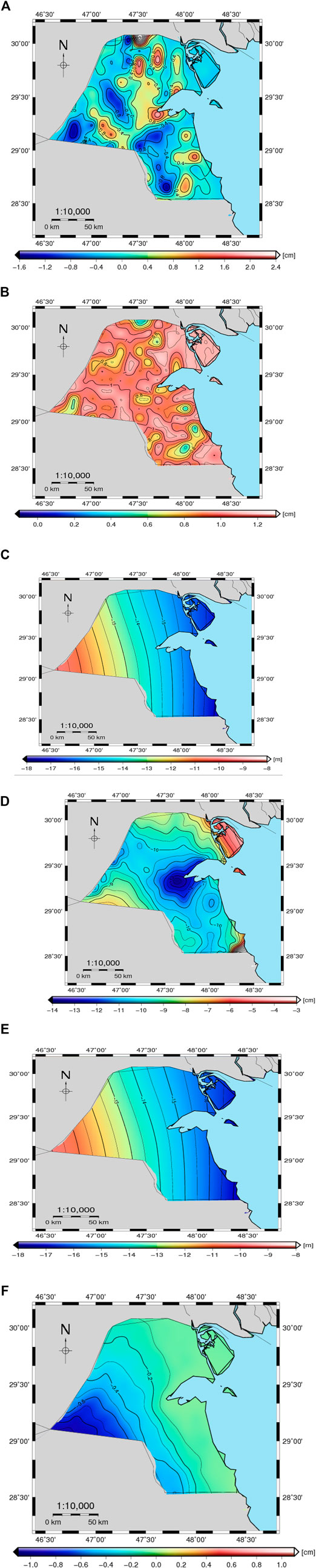
FIGURE 5. (A) The residual height anomalies (cm). (B) The estimated error of residual height anomalies (cm). (C) The XGM2019 height anomalies at d/o 2,190 (m). (D) The RTM effects on height anomalies ${\text{ζ}}_{RTM}$ (cm). (E) The gravimetric quasigeoid model (m). (F) The geoid-to-quasigeoid separation (cm).

The reference geoid model makes the most significant contribution to the gravimetric geoid model, and the ${\text{ζ}}_{GGM}$ is obtained from XGM2019 GGM at d/o 2,190 as shown in Figure 5C. Figure 5D represents the height anomalies restored from the topography effect ${\text{ζ}}_{RTM}$, which range from −13.7 to −0.7 cm with a mean of about –8.93 cm and a standard deviation of 1.83 cm.

Figure 5E shows the gravimetric quasigeoid model KW-LQGM2021. The geoid/quasigeoid separation shown in Figure 5F is at level −0.3 cm for the majority of Kuwait land, increasing to -1.1 cm on the western boundary.

Finally, the gravimetric quasigeoid model KW-LQGM2021 is converted to the geoid model KW-LGM2021 as given in Figure 6 based on Eq. 11 by adding the geoid/quasigeoid separation (Figure 5F) to the model KW-LQGM2021 (Figure 5E). Table 2 shows the statistics of the quasigeoid model KW-LQGM2021, geoid/quasigeoid separation, and the geoid model KW-LGM2021.

FIGURE 6

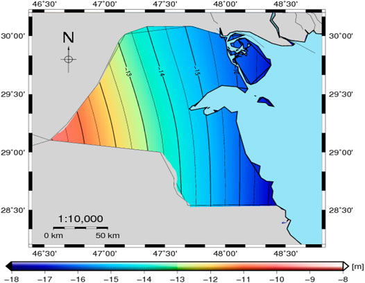
FIGURE 6. The gravimetric geoid model KW-LGM2021 (m).

TABLE 2

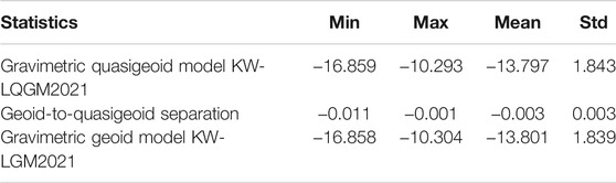
TABLE 2. Statistics of the height anomalies, geoid-to-quasigeoid separation, and geoid heights (m).

Fitting of the Gravimetric Geoid Models With the National Vertical Datum

At first, it is important to understand the difference between gravimetric geoid and GPS\leveling heights. The former geoid heights are considered a surface that is solely related to gravimetric data and has no practical geodetic application in the MSL-based vertical reference system because it is not connected to local or national height networks.

The fitted geoid model is a gravimetric geoid model that has been fitted (adjusted) to a local vertical height system. Between the ellipsoidal and orthometric heights, the fitted geoid surface is used as a transformation surface. As a result, the fitted geoid will always be tied to a specific vertical datum, such as a national local vertical datum based on mean sea level (MSL).

In this study, 83 GPS/leveling stations associated with the national local vertical datum of Kuwait state were employed by running the FITGEOID module of the GRAVSOFT software to reduce the datum shift between the derived gravimetric geoid model and the Kuwait national vertical datum (Forsberg and Tscherning, 2008).

As a result, the improved fitted geoid was achieved by utilizing a four-parameter Helmert similarity transformation model to reduce the trend surface’s datum shift between gravimetric geoid models and GPS/leveling stations, as shown in Table 3. The geoid accuracies after trend reduction (Figure 7) have been lowered from 24.4 to 8.20 cm (as shown by the standard deviation of the results).

TABLE 3

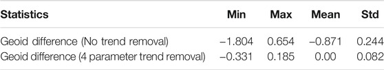
TABLE 3. Statistics of the differences between the $N_{gravimetricgeoid}$ and $N_{GPS/leveling}$ (m).

FIGURE 7

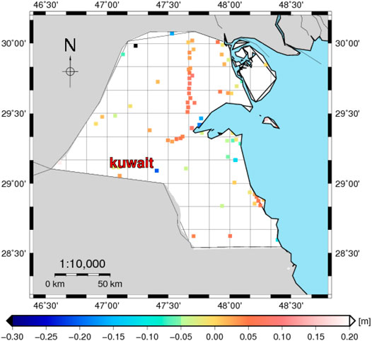
FIGURE 7. The differences between the geoid model and GPS/leveling after 4-parameter trend remove.

To remove the residual differences, only 68 GPS/leveling stations were used to fit the geoid by using LSC (see, Figure 8). The remaining 15 GPS/leveling stations (see, Figure 9) are used to evaluate the final geoid model. Table 4 shows the comparisons between the final geoid with the 68 GPS/leveling data; the results show a very good fitting process with 0.00 and 0.003 m for mean and STD, respectively.

FIGURE 8

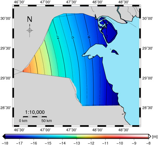
FIGURE 8. The fitted gravimetric geoid model KW-FLGM2021 after removing the bias (m).

FIGURE 9

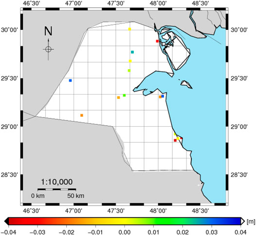
FIGURE 9. The differences between the developed fitted geoid models of Kuwait and the corresponding ones from 15 GPS/leveling data (m).

TABLE 4

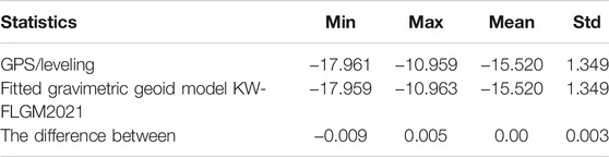
TABLE 4. Statistics of the differences between the fitted gravimetric geoid model KW-FLQGM2021 after removing the bias with the 68 GPS/leveling (m).

As shown in Table 5, the external accuracy of the final geoid KW-FLGM2021 with the 15 GPS/leveling points was extremely good, with a minimum, maximum, mean, and standard deviation of −0.038, 0.031, 0.003, and 0.022 m, respectively. For comparison, the agreement between GPS/leveling benchmarks and the XGM2019e at d/o 5,540 (without fitting) is stated as well.

TABLE 5

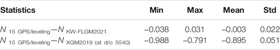
TABLE 5. Statistics of the differences between the KW-FLGM2021 model and XGM2019 with the 15 GPS/leveling stations.

The KW-FLGM2021 model outperforms the XGM2019 model by a ratio of roughly 2.2. This underlines that the KW-FLGM2021 model improves geoid heights by roughly 55% over Kuwait in comparison to XEGM2019. Furthermore, the KW-FLGM2021 model has the lowest mean geoid inaccuracy of 0.3 cm. The discrepancies between the 15 check GPS/leveling stations and XGM2019 produce mean values of about 89.5 cm.

Conclusion

In this study, a model for gravimetric geoid KW-FLGM2021 for Kuwait state has been computed using the XGM2019e up to d/o 2,190, terrestrial gravity, and SRTM3. The RCR method, with RTM topographic reduction and LSC, is used to compute the geoid model.

The study of the KW-FLGM2021 utilizing GNSS/leveling data found that the accuracy of geoid heights from the standard deviation of geoid height discrepancies is about 8.2 cm after using the four-parameter transformation model. Only 68 GPS/leveling stations were used to fit the geoid using LSC to eliminate residual discrepancies, and the remaining 15 GPS/leveling stations were utilized to validate the final geoid model. With an STD of 2.2 cm, the exterior accuracy of the final geoid KW-FLGM2021 with the 15 GPS/leveling points was exceptionally good. Overall, the KW-FLGM2021 model is recommended for use in Kuwait as a vertical reference system for leveling measurements (orthometric heights).

Data Availability Statement

The original contributions presented in the study are included in the article/Supplementary Material, further inquiries can be directed to the corresponding author.

Author Contributions

AZ and ME-A designed the study, performed the methodology research, data processing, and analysis, and drafted the manuscript. HA-A performed the GPS leveling data validation and analysis and drafted part of the manuscript. ME-A conducted the computation of RTM effect and the analysis of geoid-quasigeoid separations. MR revised the paper. All authors read and approved the final manuscript.

Conflict of Interest

The authors declare that the research was conducted in the absence of any commercial or financial relationships that could be construed as a potential conflict of interest.

Publisher’s Note

All claims expressed in this article are solely those of the authors and do not necessarily represent those of their affiliated organizations, or those of the publisher, the editors, and the reviewers. Any product that may be evaluated in this article, or claim that may be made by its manufacturer, is not guaranteed or endorsed by the publisher.

Acknowledgments

We thank our friends at Vision International Co. in Kuwait for providing us with the GPS/leveling observations that greatly aided our research, as well as to Eng. Eid Al-Aadamy, CEO of Vision Kuwait. To compute KW- FLGM2021, GRAVSOFT software modules were used (Forsberg and Tscherning, 2008). Global Mapping Tools (GMT5) have been used to plot results spatially.

References

Andersen, O., Knudsen, P., Kenyon, S., Factor, J. K., and Holmes, S. (2013). “The DTU13 Global marine Gravity Field—First Evaluation,” in Ocean Surface Topography Science Team Meeting (Springer, Cham: Boulder, Colorado).

Google Scholar

El-Ashquer, M., Al-Ajami, H., Zaki, A., and Rabah, M. (2020). Study on the Selection of Optimal Global Geopotential Models for Geoid Determination in Kuwait. Surv. Rev. 52 (373), 373–382. doi:10.1080/00396265.2019.1611256

CrossRef Full Text | Google Scholar

Ellmann, A., and Vaníček, P. (2007). UNB Application of Stokes-Helmert's Approach to Geoid Computation. J. Geodynamics 43 (2), 200–213. doi:10.1016/j.jog.2006.09.019

CrossRef Full Text | Google Scholar

Erol, B. (2007). Investigations on Local Geoids for Geodetic Applications. (Istanbul, Turkey: İstanbul Technical University). Thesis (PhD).

Forsberg, R. (1984). A Study of Terrain Reductions, Density Anomalies and Geophysical Inversion Methods in Gravity Field Modelling. Report No. OSU/DGSS-355. Ohio: Ohio State University. Dept of Geodetic Science and Surveying.

Google Scholar

Forsberg, R., and Sideris, M. G. (1993). Geoid Computations by the Multi-Band Spherical FFT Approach. Manuscripta geodaetica 18, 82.

Google Scholar

Forsberg, R., and Tscherning, C. (2008). “An Overview Manual for the GRAVSOFT Geodetic Gravity Field Modelling Programs,” in Contract Report for JUPEM. 2nd edn. Copenhagen, Denmark: National Space Institute (DUT-Space).

Google Scholar

Förste, C., Bruinsma, S., Abrikosov, O., Flechtner, F., Marty, J.-C., Lemoine, J.-M., et al. (2015). “R. Biancale, 2014, EIGEN-6C4 the Latest Combined Global Gravity Field Model Including GOCE Data up to Degree and Order 2190 of GFZ Potsdam and GRGS Toulouse. GFZ Data Services,” in EGU General Assembly Conference Abstracts.

Google Scholar

Hennig, T. A., Kretsch, J. L., Pessagno, C. J., Salamonowicz, P. H., and Stein, W. L. (2001). The Shuttle Radar Topography mission. Lecture Notes Comput. Sci. (including subseries Lecture Notes Artif. Intelligence Lecture Notes Bioinformatics) 2181 (2), 65–77. doi:10.1007/3-540-44818-7_11

CrossRef Full Text | Google Scholar

Hofmann-Wellenhof, B., and Moritz, H. (2006). Physical Geodesy. Berlin, Germany: Springer Science and Business Media.

Google Scholar

Huang, J., and Véronneau, M. (2013). Canadian Gravimetric Geoid Model 2010. J. Geod 87 (8), 771–790. doi:10.1007/s00190-013-0645-0

CrossRef Full Text | Google Scholar

Kaloop, M. R., Pijush, S., Rabah, M., Al-Ajami, H., Hu, J. W., and Zaki, A. (2021). Improving Accuracy of Local Geoid Model Using Machine Learning Approaches and Residuals of GPS/levelling Geoid Height. Surv. Rev., 1–14. doi:10.1080/00396265.2021.1970918

CrossRef Full Text | Google Scholar

Kaloop, M. R., Rabah, M., Hu, J. W., and Zaki, A. (2018). Using Advanced Soft Computing Techniques for Regional Shoreline Geoid Model Estimation and Evaluation. Mar. Georesources Geotechnology 36 (6), 688–697. doi:10.1080/1064119x.2017.1370622

CrossRef Full Text | Google Scholar

Kaloop, M. R., Zaki, A., Al-Ajami, H., and Rabah, M. (2020). Optimizing Local Geoid Undulation Model Using GPS/levelling Measurements and Heuristic Regression Approaches. Surv. Rev. 52 (375), 544–554. doi:10.1080/00396265.2019.1665615

CrossRef Full Text | Google Scholar

Knudsen, P. (1987). Estimation and Modelling of the Local Empirical Covariance Function Using Gravity and Satellite Altimeter Data. Bull. Geodesique 61 (2), 145–160. doi:10.1007/bf02521264

CrossRef Full Text | Google Scholar

Kvas, A., Mayer-Gürr, T., Krauß, S., Brockmann, J. M., Schubert, T., Schuh, W.-D., et al. (2019). “The Combined Satellite-Only Gravity Field Model GOCO06s,” in 27th IUGG General Assembly.

Google Scholar

Matsuo, K., and Kuroishi, Y. (2020). Refinement of a Gravimetric Geoid Model for Japan Using GOCE and an Updated Regional Gravity Field Model. Earth Planets Space 72 (1), 33. doi:10.1186/s40623-020-01158-6

CrossRef Full Text | Google Scholar

Moritz, H. (1978). Least-squares Collocation. Rev. Geophys. 16 (3), 421–430. doi:10.1029/rg016i003p00421

CrossRef Full Text | Google Scholar

Olson, C. J., Becker, J. J., and Sandwell, D. T. (2014). A New Global Bathymetry Map at 15 Arcsecond Resolution for Resolving Seafloor Fabric: SRTM15_PLUS. San Francisco, CA: AGUFM, OS34A–03.

Google Scholar

Pail, R., Fecher, T., Barnes, D., Factor, J. F., Holmes, S. A., Gruber, T., et al. (2018). Short Note: the Experimental Geopotential Model XGM2016. J. Geod 92 (4), 443–451. doi:10.1007/s00190-017-1070-6

CrossRef Full Text | Google Scholar

Pavlis, N. K. (2008). “An Earth Gravitational Model to Degree 2160: EGM2008,” in presented at the 2008 General Assembly of the European Geosciences Union, Vienna, Austria, April 13--18 2008.

Google Scholar

Rexer, M., Hirt, C., and Pail, R. (2017). High-resolution Global Forward Modelling: A Degree-5480 Global Ellipsoidal Topographic Potential Model. Vienna: EGUGA, 7725.

Google Scholar

Saadon, A., El-Ashquer, M., Elsaka, B., and El-Fiky, G. (2021). Determination of Local Gravimetric Geoid Model over Egypt Using LSC and FFT Estimation Techniques Based on Different Satellite- and Ground-Based Datasets. Surv. Rev., 1–11. doi:10.1080/00396265.2021.1932148

CrossRef Full Text | Google Scholar

Sansò, F., and Sideris, M. G. (2013). Geoid Determination: Theory and Methods. Berlin, Germany: Springer Science and Business Media.

Google Scholar

Schwarz, K. P. (1984). “Data Types and Their Spectral Properties,” in Local Gravity Field Approximation (Beijing, China: Beijing International Geoid Determination Summer School).

Google Scholar

Shen, W., and Han, J. (2013). Improved Geoid Determination Based on the Shallow-Layer Method: A Case Study Using EGM08 and CRUST2. 0 in the Xinjiang and Tibetan Regions. Terrestrial, Atmos. Oceanic Sci. 24 (4), 591. doi:10.3319/tao.2012.11.12.01(tibxs)

CrossRef Full Text | Google Scholar

Sjöberg, L. E. (2003). A Computational Scheme to Model the Geoid by the Modified Stokes Formula without Gravity Reductions. J. Geodesy 77 (7–8), 423–432. doi:10.1007/s00190-003-0338-1

CrossRef Full Text | Google Scholar

Torge, W., and Müller, J. (2012). Geodesy. Berlin, Germany: Walter de Gruyter.

Google Scholar

Tscherning, C. C. (2013). “Geoid Determination by 3D Least-Squares Collocation,” in Geoid Determination (Berlin, Germany: Springer), 311–336. doi:10.1007/978-3-540-74700-0_7

CrossRef Full Text | Google Scholar

Tscherning, C. C., and Rapp, R. H. (1974). Closed Covariance Expressions for Gravity Anomalies, Geoid Undulations, and Deflections of the Vertical Implied by Anomaly Degree Variance Models. Ohio: Scientific Interim Report Ohio State Univ.

Google Scholar

Varga, M., Pitoňák, M., Novák, P., and Bašić, T. (2021). Contribution of GRAV-D Airborne Gravity to Improvement of Regional Gravimetric Geoid Modelling in Colorado, USA. J. Geodesy 95 (5), 1–23. doi:10.1007/s00190-021-01494-9

CrossRef Full Text | Google Scholar

Zaki, A. (2015). Assessment of GOCE Models in EgyptMaster Thesis. Egypt: Faculty of engineering, Cairo university.

Google Scholar

Zaki, A., and Mogren, S. (2021). A High-Resolution Gravimetric Geoid Model for Kingdom of Saudi Arabia. Surv. Rev., 1–16. doi:10.1080/00396265.2021.1944544

CrossRef Full Text | Google Scholar

Zaki, A. (2018). Satellite Gradiometry for Modeling Sea Current Circulation (Zagazig, Egypt: Faculty of Engineering, Zagazig University). Phd Thesis. doi:10.13140/RG.2.2.23704.14087

CrossRef Full Text

Zingerle, P., Pail, R., Gruber, T., and Oikonomidou, X. (2020). The combined global gravity field model XGM2019e. J. Geod 94 (7), 66. doi:10.1007/s00190-020-01398-0

CrossRef Full Text | Google Scholar