 Chongjin Zhao
 Luolei Zhang
 Peng Yu1
 Xi Xu
Xi Xu- 1State Key Laboratory of Marine Geology, Tongji University, Shanghai, China
- 2China Aero Geophysical Survey and Remote Sensing Center for Natural Resources, Beijing, China
The Songpan−Aba region is located on the northeastern edge of the Tibetan Plateau. Tectonically, the area is surrounded by the West Qinling orogenic belt in the north, the Longmenshan orogenic belt in the southeast, and the East Kunlun and Sanjiang orogenic belts in the west and southwest, forming a triangle that provides an ideal location to study the crust-mantle structure and deep tectonics of the eastward extrusion of the Tibetan Plateau. In this study, the magnetic and electrical structures of the Songpan−Aba area were investigated by inversion using high-precision magnetic anomaly and magnetotelluric data to obtain the subsurface magnetization inversion intensity and resistivity of Songpan–Aba and adjacent areas. The results revealed a continuous magnetic layer up to 20 km below Songpan–Aba and its surrounding areas in the south, possibly originating from a magma root southwest of the Longmenshan massif. In the West Qinling, Songpan–Aba, and Longmenshan areas, pervasive low-resistance, weakly magnetic, or magnetic layers were identified below 20 km that might be formed from the molten mantle material extruded from the eastern edge of the Tibetan Plateau.
Introduction
Songpan–Aba is located at the northeastern edge of the Tibetan Plateau (Figure 1) and situated at the interface of the east–west and north−south tectonic components of China. It is an important region for studying the eastward extrusion of crustal material from the Tibetan Plateau (Tapponnier et al., 1982).
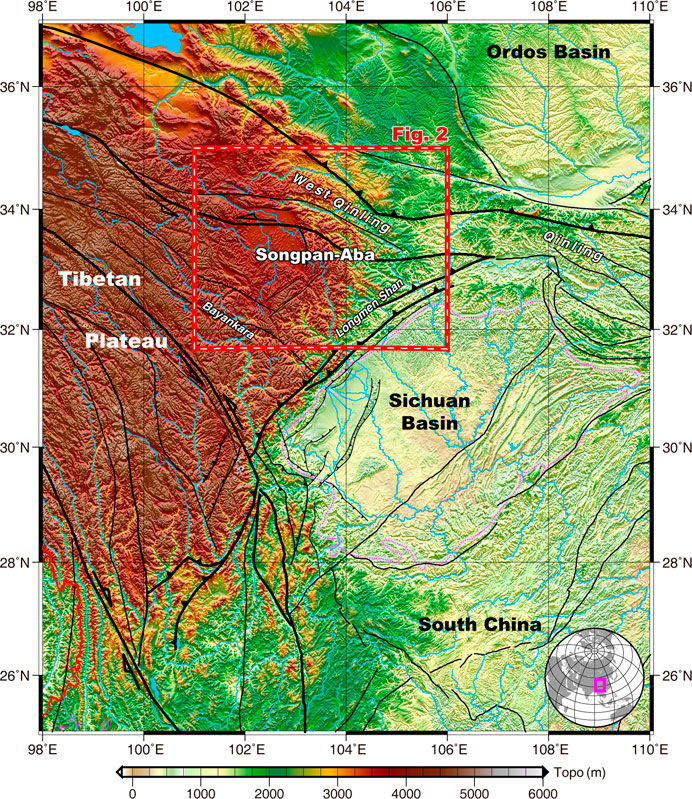
FIGURE 1. Location of the study area (red box).
Since the 1980s, several studies have proposed deformation models to explain the eastern Tibetan Plateau uplift. The first was the rigid block model, which concluded that the uplift of the eastern Tibetan Plateau could be primarily attributed to the deformation of brittle substances in the crust caused by thrust nappe (Tapponnier and Molnar, 1976, 1982, 2001; Avouac and Tapponnier, 1993); the second was the continuous deformation model (England and Dan, 1985, 1986, 2010; Houseman and England, 1986); and the third was the crustal flow model, which proposed that a low-viscosity asthenosphere in the lower crust of the eastern Tibetan Plateau slid eastward under plate movement and was blocked by the Sichuan Basin, resulting in the accumulation and lift of a lower crustal substance with low velocity and high conductivity (Bird, 1991; Royden et al., 1997; Royden et al., 1977; Clark and Royden, 2000).
Seismic tomography studies (Wang et al., 2005; Wang, 2007; Wu et al., 2009), receiver functions (Liu et al., 2015), and environmental noise imaging (Yang et al., 2013) of the Tibetan Plateau concluded that crustal and upper mantle structures in the eastern margin of the Tibetan Plateau were different from those in its surrounding regions, such as the Sichuan Basin and the South China Plate. The seismic wave velocity indicated a relatively steep gradient change at the junction of the Tibetan Plateau, its surrounding plates, and middle and lower crustal flows in the northeastern Tibetan Plateau (Pan et al., 2017).
Magnetotelluric (MT) is an important method to probe the deep structure of the lithosphere and can effectively reveal the distribution of subsurface fluids. Several MT studies conducted in the eastern periphery of the Tibetan Plateau have elucidated the electrical structure of the regional crust and mantle, showing expansive low-resistance layers widely distributed in the middle and lower crust of the northeastern margin (Sun et al., 2003; Xu et al., 2007; Zhao et al., 2008; Wang et al., 2009, 2013; Zhang et al., 2012; Bai et al., 2013), indicating the prevalent presence of fluids and local melting. Their distribution characteristics were consistent with the “crustal flow” model, providing strong evidence for it from the perspective of conductive structures (Li et al., 2017).
The regional magnetic anomalies were primarily due to highly magnetized crustal rocks that provided information on crustal composition and structural variations beneath the Earth’s surface (Wang et al., 2020). Previous studies in this area did not adopt the combined magnetic and MT approach to investigate subsurface tectonics. Therefore, this study aimed to apply high-precision magnetic survey data to conduct magnetization intensity inversion in Songpan–Aba and adjacent areas to obtain three-dimensional (3D) regional magnetic properties. Meanwhile, the subsurface electrical structure was derived from four high-precision MT profiles collected over a long period to analyze the deep structure of the Songpan–Aba area from subsurface magnetic and electrical property perspectives, and to further examine the deep geological structures of the eastern margin of the Tibetan Plateau.
Methods
Magnetic Inversion Process
3-D Inversion of Total-Field Magnetic Anomalies
The non-uniqueness and instability of the solutions have typically focused on previous magnetic anomaly inversion studies, as they are important factors restricting magnetic inversion development. Tikhonov and Arsenin (1977) proposed the regularization theory to solve such problems. The forward sum function, A, decreases rapidly with increasing depth, yielding an inversion result near the ground (Li and Oldenburg, 1998; Zhdanov, 2002). The depth weighting of this regularization method depends on the selection of the regularization factor, α. The adaptive regularization factor selection method proposed by Hu et al. (2019) was applied in this study. We followed Li and Oldenburg (1996), using the reciprocal of the vertical surface component of the total magnetic anomaly data as the data-weighting factor. If the model sensitivity matrix is directly incorporated into data-fitting (Zhdanov, 2002; Hu et al., 2019; Zhao et al., 2020), this problem can be solved. After model weighting, the total sensitivities of the weighted model parameter of all grid cells are equal, and the contribution of observed data is essentially identical. The objective function is defined as follows:
where ϕ(mw) is the data-fitting function and S (mw) is the model-stabilizing function.
The model weighted matrix (Wm) is:
where
The uniqueness of the 3-D inversion of the total-field magnetic anomalies is the forward operator, A, with different magnetic inclination and declination in different grids (Bhattacharyya, 1964).
where
If there is no remanence, and assuming that the inclination (I0) and declination (D0) of each data grid are known, then the oblique magnetization forward matrix A can be directly calculated. In this study, the inclination and declination were directly incorporated into the total magnetic intensity inversion process, ΔT.Zhdanov (2002) reported the iteration process of the conjugate gradient.
Magnetic Data
High-precision magnetic anomaly data were acquired in the study area using five G-856 and four G-858 magnetometers. We set up nine magnetic observation stations for diurnal variations in Jiangyou, Shuijingbao, Sedi, Lianghekou, Hongyuan, Jiuzhi, Maqu, Diebu, and Dangchang to adequately and effectively control the measurement area and improve the accuracy of each measurement point. The locations were free from human interference and active magneticity, with the convenience of use, clear markings, and accessible storage. Joint measurements were conducted at these stations from 5–8 am and 5–10 pm (when the magnetic field was relatively stable) to achieve magnetic field normalization. The data recorded during these two periods were used to obtain the basic magnetic field value of the observation stations. The radius for the joint measurements was controlled to within 50 km. The data collected included the total magnetic anomaly △T, with a total root-mean-square error of the magnetic measurements <5nT. The field survey was set up with 13 survey lines spaced 30 km apart. The measurement points were arranged on each line at 2-km intervals, resulting in 1,985 points (see Table 1).
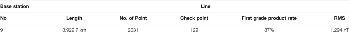
TABLE 1. Summary of magnetic data.
Data from other areas were collated and supplemented using Satellite Magnetic Anomaly Data (https://www.ngdc.noaa.gov/geomag/emag2.html) (Figure 2A) from the Earth Magnetic Anomaly Grid (EMAG2) database published by the Commission for the Geological Map of the World (Maus et al., 2009). This database of crustal magnetic anomalies was accumulated from airborne, offshore, and satellite magnetic surveys over 50 years at a 2’ × 2’ global grid resolution. As shown by the magnetic anomaly map of the Songpan–Aba area, the object under investigation in this study was characterized by stable weak magnetic anomalies, varying from −30 to −50 nT in a steady, smooth magnetic field. The magnetic field in the eastern part of the survey area varied drastically with local anomalies. The measurement area was divided into the following zones according to the strength of the magnetic anomalies:
1) North China plate: This region exhibited varying positive and negative magnetic anomalies. Numerous rock outcrops primarily formed in the Indosinian period, and a some formed during the Hercynian and Yanshanian periods, exist in this region. The distribution of exposed rocks was well correlated with the magnetic anomalies. The magnetic anomaly was in the north-northeast direction and positive, with the highest value >200 nT. The rocks formed during the Indosinian period exhibited various magnetic properties, ranging from weak to strongly magnetic, with their magneticity related to the magnetic minerals content of the rocks. The ferromagnetic mineral content is low in acidic rocks, which exhibit weak to moderate magneticity, whereas intermediate mafic rocks are more magnetic and show high magnetic anomalies.
2) West Qinling area: This area revealed broad, smooth negative magnetic anomalies stacked with local magnetic anomalies. The magnetic anomaly in this area was characterized as low, with some local high magnetic spots. The background value of the low negative magnetic anomaly was approximately −40 nT and the stacked local anomalies were higher overall than the background anomaly value.
3) Longmenshan and Bayankara massifs: The anomalies of the Longmenshan and Bayankara massifs showed the lowest magnetic anomaly distribution in the study area, with the magnetic anomalies ranging from −80 to −200 nT. The magnetic anomalies gradually intensified from the Sichuan Basin in the southeast to the northwest corners of the area. Only one north−east trending high-positive magnetic anomaly with a maximum value of ∼160 nT occurred near Jiangyou and a 200 nT anomaly appeared north of Guangyuan. The overall orientation of magnetic anomalies in this area was north−east trending, with dense anomaly contours and rapid gradient changes between the negative anomalies.
4) The Songpan–Aba crust was a stable zone of low, negative magnetic anomalies of approximately −40 nT, with ∼10 nT fluctuations. The anomalies decreased to approximately −50 nT eastwards at Nanping.
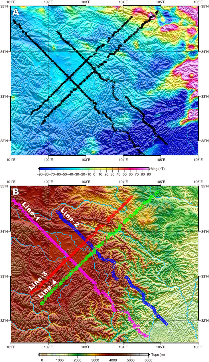
FIGURE 2. Magnetic anomalies in study area (A) and Magnetotelluric survey lines (B) (pink triangle is Line 1, blue square is Line 2, red triangle is Line 3 and green square is Line 4).
Three-Dimensional Magnetic Structure
First, a theoretical model was designed to verify the practicality and stability of the proposed algorithm, then a model consisting of three blocks of different depths and sizes was designed, as shown in (Figure 3A). The model space was 40 × 40 × 21 grid cells, that were each 1 × 1 × 1 km in size, and the magnetization of the model was 1 A/m. Figure 3B shows the synthetic data with the I0 = 52°and D0 = −1°, where the data space was 40 × 40 grid cells, and each cell was 1 × 1 km. A profile selected in this study is indicated by the pink line in Figure 3B. Regularized inversion was then performed, and the results are shown in Figure 3C. The profile was selected for a detailed comparison of the model and inversion results, as indicated in Figure 3D.
FIGURE 3. Theoretical Magnetization model of three-blocks model: (A) True model; (B) The oblique magnetic anomaly at an inclination of 52° and declination of –1°(the black boxes indicate the true positions of the abnormal body, the pink line indicates the profile); (C) the iso-surface of Magnetization inversion result (M = 0.5A/m); (D) the profile of the inversion result (the black boxes indicate the true positions of the abnormal body).
Further, the number of grids in the east–west, north–south, and vertical directions were 97, 81, and 40, respectively, for the 3D inversion of the measurement data obtained from the 5 × 5 km horizontal-dimension grids in the study area. The vertical depth of the forward modeling and inversion was on average, divided into 40 grids covering 40 km (the vertical interval for the grid is 1 km). One hundred iterations were performed in the inversion, in which the data-fitting error was reduced from an initial value of six root-mean-square (RMS) to approximately two RMS. Figure 4 shows the results of the regularized inversion based on the weighted model. We derived the trend and distribution of the magnetic anomaly in the study area from the iso-surface images.
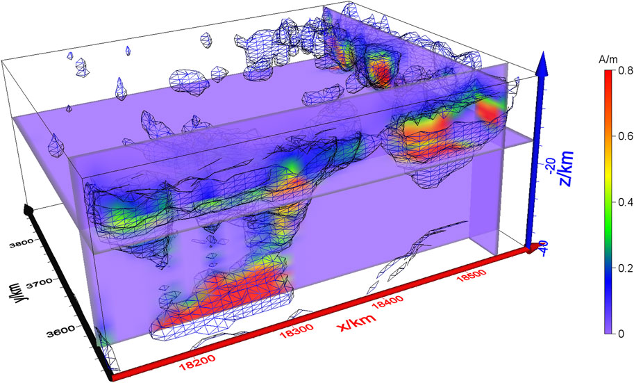
FIGURE 4. Three-dimensional joint inversion of oblique magnetization. M = 0.1 A/m iso-surface image (Z axis is the number of grids, and one grid represents 2 km).
MT Inversion Process
MT-Regularized Inversion
A method for solving the non-uniqueness of geophysical inverse problems is described in the Tikhonov and Arsenin (1977) regularization theory that uses both data misfit and a model-stabilizing functional to construct the parametric objective functional. The objective functional of the regularized inversion can be written as
where p (m,d) is the parametric objective functional, m is a vector consisting of model parameters, A(m) is the forward operator, d is a vector containing the observation data, ||·|| is the L2-norm, φ(m) is the model-stabilizing functional, and α is the regularization parameter.
A stabilizing functional is used to select the appropriate class of models from the model space of all possible models that are a correction set for solving the inverse problem (Zhdanov, 2002). The minimum support (MS) stabilizing functional was proposed to obtain a model that minimizes the volume with anomalous model parameters to improve the resolution of the sharp electrical interface (Last and Kubik, 1983). It focuses on where/how the model parameters are different with respect to the given a priori model. Here, the MS stabilizing functional can be expressed as
Xiang et al. (2017) and Zhang et al. (2020) analyzed the advantages and disadvantages of several commonly used families of stabilizing functionals, such as the smooth, MS or minimum gradient support (MSG). We then applied a new stabilizing functional, the MSG that combines smooth and sharp-boundary constraints with a unified form for the objective functional in the 2-D regularized inversion. The MSG stabilizing functional is defined as:
The spatial gradient is calculated after the MS stabilizer is obtained using Eq. 3, thus, we refer to this new stabilizing functional as the MSG, which uses an MS value instead of m—mapr, leading to a stable constraint that focuses on sharp boundaries for inversion. This functional acts on the class of models such as the domain with an anomalous parameter distribution that occupies the minimum volume, while avoiding any instability caused by simultaneously focusing parameter tuning. The MSG stabilizing functional is minimally affected by the a priori model. Zhdanov (2002) proved that the MS and MGS satisfy the Tikhonov criterion for a regularization stabilizer. Since the MSG is a spatial gradient of the MS, it also satisfies the regularization criterion.
Data Sources
Four survey lines (Lines 1, 2, 3, and 4) were identified for MT data acquisition in the Songpan–Aba area. Lines one and two were parallel and trending in a SE−NW direction with an ∼45° azimuth, whereas Lines three and four were trending in an SW−NE direction with the same azimuth. The survey lines spanned the entire Songpan–Aba area. Field testing was conducted using Model V-2000 devices in a five-component tensor-impedance format, in 2002. In total, 809 points were collected from the 4 MT profiles in the region. The detailed line layout and workload requirements are shown in Figure 2B and Table 2, respectively. The survey was fully implemented using fixed-station and remote-reference methods throughout the survey area. The effective recording bands were 320–0.001 Hz, the electrode distance was 100 m, and the ground resistance was <1 KΩ. The horizontal magnetic rods were buried below 50 cm and the vertical magnetic rods were inserted approximately three-quarters into the ground. Differential GPS positioning was applied to determine the locations of the survey points, maintaining the precision of the plane coordinates within ±10 m. The measurement network was maintained in a regular form, with point distance and lateral deviations within 400 m. Maintenance was conducted to ensure that at least 85% of the physical points were working during the survey.
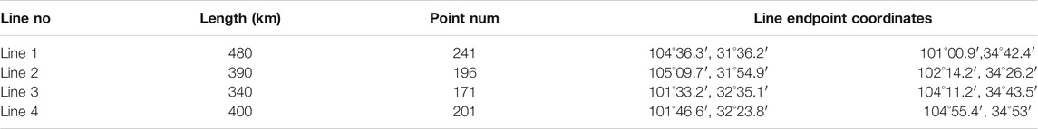
TABLE 2. MT profile workload table.
Electrical Conductivity Structure
First, a theoretical model was designed (Figure 5A) with the resistivity of wall rock at 100 Ω m and the resistivity of a high-conductivity strip at 5 Ω m. The above-mentioned two-dimensional MT-regularized inversion method, with inversion parameters based on the constraints of the MSG model, was used to perform the inversion for this theoretical model. The horizontal grids were set up on a 10-km scale and the vertical grids were divided into 86 layers, which were equally spaced in a log scale up to 300 km. The model response incorporated 5% Gaussian random noise, with 40 frequencies from 320–0.00055 Hz. The initial model was an infinite half-space of 100 Ω m. The inversion results are shown in Figure 5B, which illustrates that the resistivity and distribution of the high-conductivity strip can be accurately delineated in the model, with the fitting error of the inversion data reduced to 1.06.
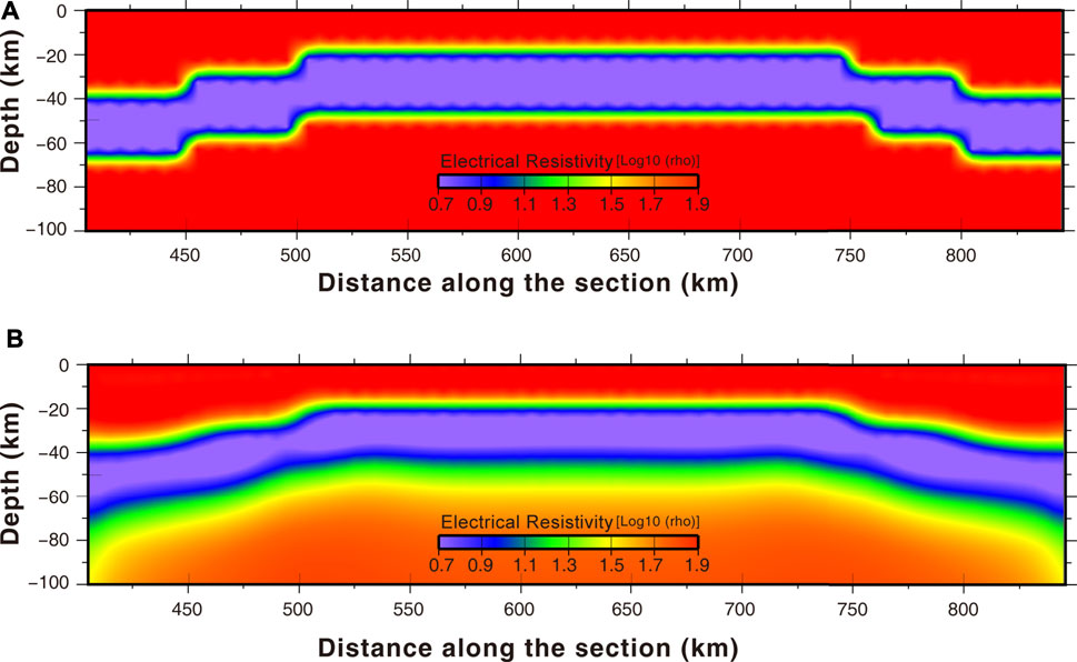
FIGURE 5. Theoretical model of high-conductivity strip: (A) True Model and (B) Inversion result.
Further, this two-dimensional MT-regularized inversion method was applied to the inversion of the four profiles in the Songpan area. The inversion parameters were as follows: the horizontal grid-scale was the spacing of the measurement points, and the vertical grids were divided into 86 layers, which were equally spaced in a log scale up to 300 km. The maximum number of iterations in the inversion was 50, and the error level was 5% (i.e., errors with an initial value < 5% were set to 5%, while >5% remained unchanged). The initial model was an infinite half-space of 100 Ω m. The four profiles converged to 1.5, 1.8, 1.3, and 1.2, respectively, using the chi-square test error as the convergence criterion. As shown in Figures 6−9 B, the resistivity structure of the four profiles revealed a vertical distribution of high-resistance-low-resistance-high-resistance. A high-resistance layer ∼20 km thick existed in the shallow ground, composed of sedimentary materials and substances from the upper crust. A high-conductivity layer was located 20–60 km below the study area, while heterogeneous high-resistance and high-conductivity anomalies appeared below 60 km. A connection was found between the high-conductivity layer (20–60 km) and the high-conductivity anomalies below 60 km; therefore, it was concluded that the high-conductivity layer between 20 and 60 km might be formed by a substance from the deep mantle which was brought to the crust through upwelling channels. A comprehensive elaboration on this conclusion, integrating the magnetic anomaly inversion results will be presented in the following section.
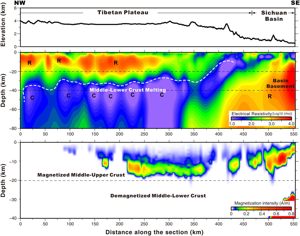
FIGURE 6. Line one magnetotelluric survey profile and magnetization distribution: (A) altitude (B) electrical resistivity and (C) magnetization distribution.
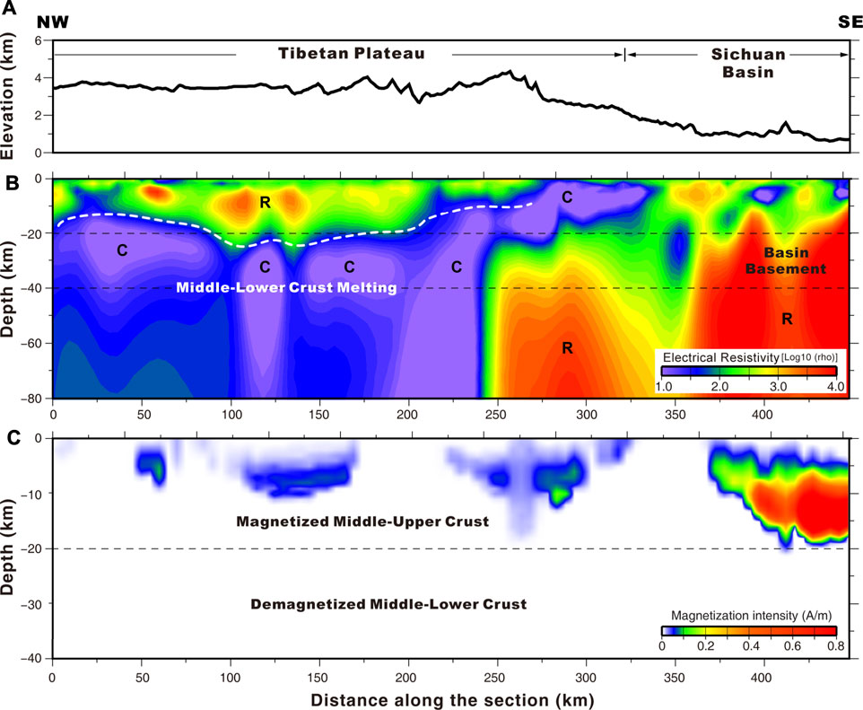
FIGURE 7. Line two magnetotelluric survey magnetization distribution profile: (A) altitude (B) electrical resistivity and (C) magnetization distribution.
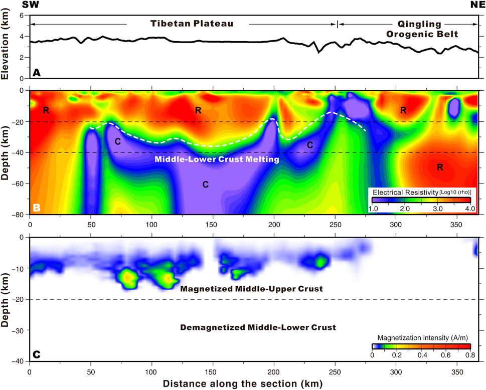
FIGURE 8. Line three magnetotelluric survey magnetization distribution profile: (A) altitude (B) electrical resistivity and (C) magnetization distribution.
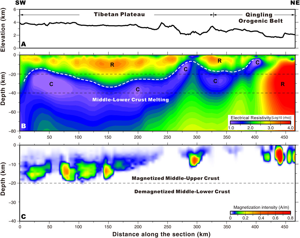
FIGURE 9. Line four magnetotelluric survey magnetization distribution profile: (A) altitude (B) electrical resistivity and (C) magnetization distribution.
Analysis and Interpretation
First, the planar distribution of magnetization intensity was extracted from the 3D magnetic results at different depths (10, 15, 20, and 30 km) (Figure 10) for the comparison of resistivity and magnetic structure among the 4 MT survey lines (Figures 6−9) to analyze the magnetic and electrical resistivity structure of the study area and its geological features.
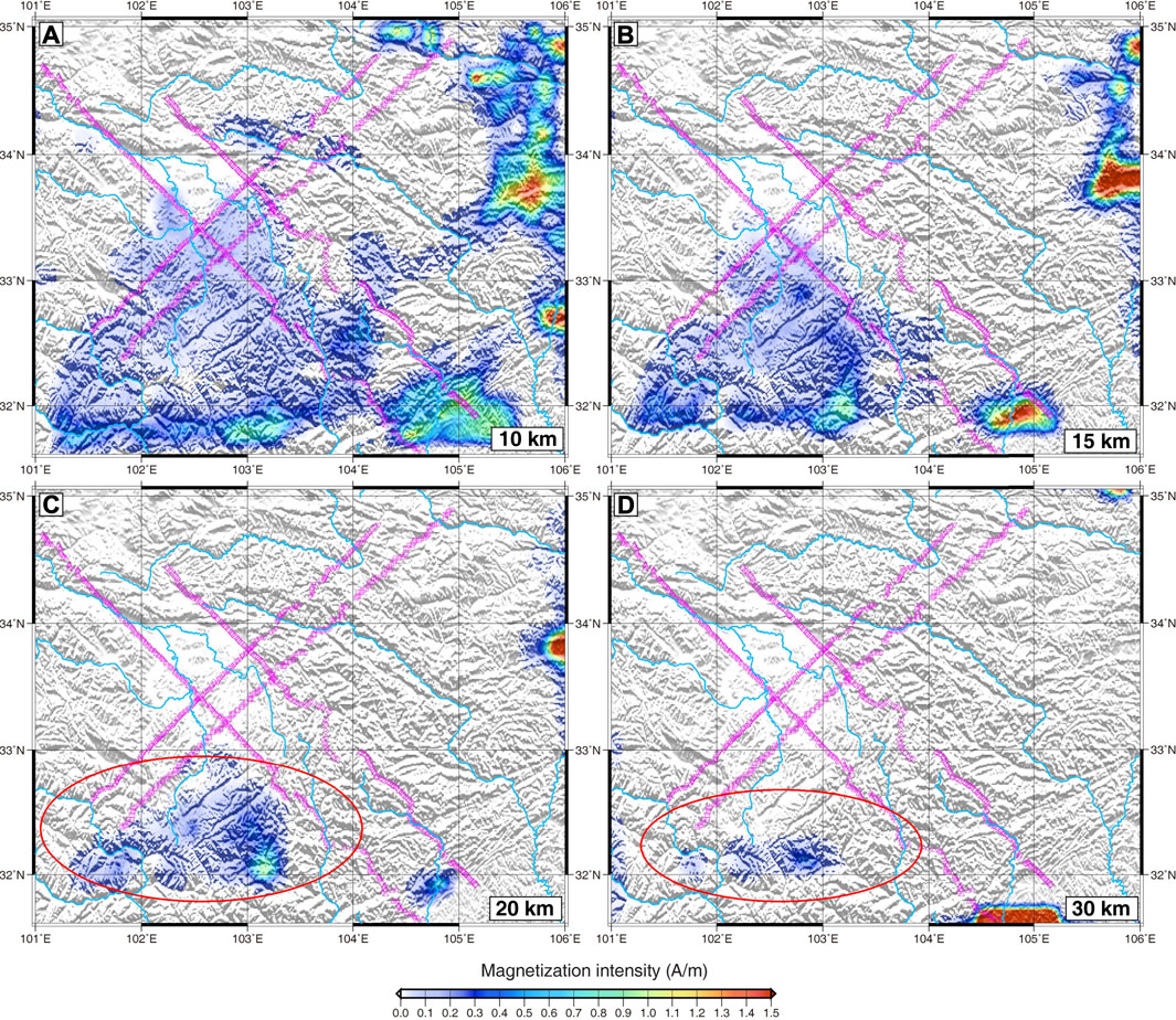
FIGURE 10. Songpan−Aba area magnetization map: (A) 10 km (B) 15 km (C) 20 km, and (D) 30 km.
The 10-km magnetization map showed that highly magnetic matter existed in the South China plate, the eastern part of the West Qinling Mountains, Sichuan, and the southern part of the Longmenshan massif, where a wide range of primarily Indosinian period rock outcrops were shown on the surface, with a small quantity from the Hercynian and Yanshanian age. The distribution of exposed rock adequately corresponded to the magnetic anomaly. The distribution of weakly magnetic substances was identified in the southwestern parts of the Songpan–Aba massif, Bayankara, and the Longmenshan massif, whereas the major parts of the West Qinling and Longmenshan massif did not contain substantial magnetic structures.
Next, from the 15–30 km magnetization map, it was observed that the magnetic bodies became significantly fewer and smaller, with only one magnetic body detected in the southern part of the Longmenshan massif at 20 km deep. The magnetic layers in the study area were distributed above 20 km. The lower boundary of a magnetic body is determined by the depth of the Curie isotherm. Temperature increases with depth, and when the temperature exceeds the Curie point of the enclosed ferromagnetic minerals (primarily magnetite in the crust), they become paramagnetic and no longer generate magnetic anomalies. The Curie temperature of magnetite in the crust is ∼580°C; therefore, the 580°C isotherm is approximately located at the bottom interface of the deep magnetic anomaly. The upper and lower boundary conditions based on the upper mantle temperature are estimated by surface temperature and the S-wave velocity from ground stations. Sun et al. (2013) estimated that the typical temperature range was 800–1,000 °C for the Moho below the Tibetan Plateau, while the thermal profile of 90°E, 30°N in southern Tibet indicated that the Curie isotherm depth was ∼20 km, consistent with our magnetic inversion results.
Figure 4 illustrates a magnetic connection linking the upper and lower compartments in the southern part of the Longmenshan massif. It was tentatively deduced that the magnetic source in the Songpan–Aba area originated from a magma root in the southwestern part of the Longmenshan massif (red circles in Figures 10C,D).
Beneath the northeastern part of the Tibetan Plateau (West Qinling, Songpan−Aba, and Longmenshan Mountains), we found an extensive low-resistance layer below 20 km that showed no magneticity, possibly due to partial melting of the crust, which might have been sourced from the substance extruded from the eastern margin of the Tibetan Plateau that was pushed eastwards under the south−north compression from the Indian and the North China plate. Subsequently, blocked by the Sichuan Basin, the lower crustal low-resistance substance congregated and lifted near the Longmenshan area, contributing to the crustal uplift, consistent with the crustal flow model (Royden et al., 1977; Clark and Royden, 2000).
Conclusion
In this study, the magnetic and electrical structures of the Songpan–Aba area were obtained from 3D oblique magnetization and MT regularization inversion using high-precision total magnetic anomalies and four long-term MT survey lines. Furthermore, we explored the origin of the magnetic layer in the southern part of the study area and the formation of zones in the northern area with or without weak magneticity.
1) A continuous magnetic layer exists above depths of 20 km under Songpan–Aba and adjacent areas on the south; it is located above the low-resistance layer in the crust and can be traced to the west side of Songpan, deepening in the northwestern part of the Longmenshan area, and possibly originating from a magma root in the southwestern part of the Longmenshan massif.
2) There are extensive low-resistance and weakly magnetic layers below 20 km in the West Qinling, Songpan–Aba, and Longmenshan areas that may be partially molten crustal material sourced from substance extruded from the eastern edge of the Tibetan Plateau.
Data Availability Statement
The original contributions presented in the study are included in the article/supplementary material, further inquiries can be directed to the corresponding author.
Author Contributions
CZ performed the experiment, the data analyses and wrote the article. LZ contributed significantly to analysis and article preparation. PY performed the analysis with constructive discussions. XX performed the analysis with constructive discussions and plotted the figures.
Conflict of Interest
The authors declare that the research was conducted in the absence of any commercial or financial relationships that could be construed as a potential conflict of interest.
Publisher’s Note
All claims expressed in this article are solely those of the authors and do not necessarily represent those of their affiliated organizations, or those of the publisher, the editors and the reviewers. Any product that may be evaluated in this article, or claim that may be made by its manufacturer, is not guaranteed or endorsed by the publisher.
Acknowledgments
We acknowledge the support from the National Natural Science Foundation of China (42074079, 41806065, 41902202), the Natural Science Foundation of Shanghai (20ZR1462300), the Key Laboratory of Airborne Geophysics and Remote Sensing Geology Ministry of Natural Resources (2020YFL13), and China Postdoctoral Science Foundation (2019M652062). Data processing and plot illustrating were supported by GMT package (https://www.generic-mapping-tools.org/).
References
Avouac, J.-P., and Tapponnier, P. (1993). Kinematic Model of Active Deformation in central Asia. Geophys. Res. Lett. 20, 895–898. doi:10.1029/93gl00128
Bai, D. H., Unsworth, M. J., Meju, M. A., Ma, X., Teng, J., Kong, X., et al. (2013). Crustal Deformation of the Eastern Qinghai-Tibet Plateau Revealed by Magnetotelluric Imaging. Nat. Geosci. 3, 358–362. doi:10.1038/ngeo830
Bhattacharyya, B. K. (1964). Magnetic Anomalies Due to Prism‐Shaped Bodies with Arbitrary Polarization. Geophysics 29, 517–531. doi:10.1190/1.1439386
Bird, P. (1991). Lateral Extrusion of Lower Crust from under High Topography in the Isostatic Limit. J. Geophys. Res. 96, 275–210. doi:10.1029/91jb00370
England, P., and Dan, M. (2010). A Thin Viscous Sheet Model for continental Deformation. Geophys. J. R. Astron. Soc. 73, 523–532. doi:10.1111/j.1365-246X.1982.tb04969.x
England, P., and Houseman, G. (1986). Finite Strain Calculations of Continental Deformation: 2. Comparison with the India-Asia Collision Zone. J. Geophys. Res. 91, 3664–3676. doi:10.1029/jb091ib03p03664
England, P., and Houseman, G. (1985). Role of Lithospheric Strength Heterogeneities in the Tectonics of Tibet and Neighbouring Regions. Nature 315, 297–301. doi:10.1038/315297a0
Houseman, G., and England, P. (1986). Finite Strain Calculations of continental Deformation: 1. Method and General Results for Convergent Zones. J. Geophys. Res. 91, 3651–3663. doi:10.1029/jb091ib03p03651
Hu, M., Yu, P., Rao, C. F., Zhao, C. J., and Zhang, L. L. (2019). 3D Sharp-Boundary Inversion of Potential-Field Data with an Adjustable Exponential Stabilizing Functional. Geophysics 84, J1–J15. doi:10.1190/geo2018-0132.1
Kristen Clark, M., and Handy Royden, L. (2000). Topographic Ooze: Building the Eastern Margin of Tibet by Lower Crustal Flow. Geology 28, 703–706. doi:10.1130/0091-7613(2000)028<0703:tobtem>2.3.co;2
Last, B. J., and Kubik, K. (1983). Compact Gravity Inversion. Geophysics 48, 713–721. doi:10.1190/1.1441501
Li, J., Wang, X. B., Li, D. H., Qin, Q-Y., Zhang, G., Zhou, J., et al. (2017). Characteristics of Lithosphere Physical Structure in the Eastern Margin of the Qinghai-Tibet Plateau and Their Deep. Chin. J. Geophys. 60, 2500–2511. (in Chinese). doi:10.6038/cjg20170637
Li, Y., and Oldenburg, D. W. (1998). 3-D Inversion of Gravity Data. Geophysics 63, 109–119. doi:10.1190/1.1444302
Li, Y., and Oldenburg, D. W. (1996). 3-D Inversion of Magnetic Data. Geophysics 61, 394–408. doi:10.1190/1.1443968
Liu, Z., Park, J., and Rye, D. M. (2015). Crustal Anisotropy in Northeastern Tibetan Plateau Inferred from Receiver Functions: Rock Textures Caused by Metamorphic Fluids and Lower Crust Flow?. Tectonophysics 661, 66–80. doi:10.1016/j.tecto.2015.08.006
Pan, J. T., Li, Y. H., Wu, Q. J., Ding, Z. F., and Yu, D. X. (2017). Phase Velocity Maps of Rayleigh Wave Based on a Dense Coverage and Portable Seismic Array in NE Qinghai-Tibet Plateau and its Adjacent Regions. Chin. J. Geophys. 60, 2291–2303. (in Chinese). doi:10.6038/cjg20170621
Royden, L. H., Burchfiel, B. C., King, R. W., Wang, E., Chen, Z., Shen, F., et al. (1997). Surface Deformation and Lower Crustal Flow in Eastern Tibet. Science 276, 788–790. doi:10.1126/science.276.5313.788
Sun, J., Jin, G. W., and Bai, D. H. (2003). Sounding of Electrical Structure of the Crust and Upper Mantle along the Eastern Border of Qinghai-Tibet Plateau and its. Sci. China (S. D) 33, 173–180 (in Chinese). doi:10.1360/03dz0019
Sun, Y. J., Dong, S. W., Fan, T. Y., Zhang, H., and Shi, Y. L. (2013). 3D Rheological Structure of the continental Lithosphere beneath China and Adjacent Regions. Chin. J. Geophys. 56, 2936–2946. (in Chinese). doi:10.1002/cjg2.20052
Tapponnier, P., and Molnar, P. (1976). Slip-line Field Theory and Large-Scale continental Tectonics. Nature 264, 319–324. doi:10.1038/264319a0
Tapponnier, P., Peltzer, G., Le Dain, A. Y., Armijo, R., and Cobbold, P. (1982). Propagating Extrusion Tectonics in Asia: New Insights from Simple Experiments with Plasticine. Geology 10, 611. doi:10.1130/0091-7613(1982)10<611:petian>2.0.co;2
Tikhonov, A. N., and Arsenin, V. Y. (1977). Solutions of Ill-Posed Problems. Washington, DC: Winston.
Wang, C. Y. (2007). Crustal Structure beneath the Eastern Margin of the Qinghai-Tibet Plateau and its Tectonic Implications. J. Geophys. Res. Solid Earth. 112, 1–21. doi:10.1029/2005JB003873
Wang, J., Yao, C. L., and Li, Z. L. (2020). Aeromagnetic Anomalies in central Yarlung-Zangbo Suture Zone (Southern Tibet) and Their Geological Origins. J. Geophys. Res. Solid Earth. 125, e2019. doi:10.1029/2019jb017351
Wang, X. B., Luo, W., Zhang, G., Cai, X. L., Qin, Q. Y., and Luo, H. Z. (2013). Electrical Resistivity Structure of Longmenshan Crust-Mantle Under Sector Boundary. Chin. J. Geophys. 56, 2718–2727. (in Chinese). doi:10.6038/cjg20130820
Wang, X. B., Zhu, Y. T., Zhao, X. K., Yu, N., Li, K., and Gao, S. Q. (2009). Deep Conductivity Characteristics of the Longmen Shinto, Eastern Qinghai-Tibet Plateau. Chin. J. Geophys. 52, 564–571. (in Chinese).
Wang, Y.-X., Mooney, W. D., Han, G.-H., Yuan, X.-C., and Jiang, M. (2005). Crustal P-Wave Velocity Structure from Altyn Tagh to Longmen Mountains along the Taiwan-Altay Geoscience Transect. Chin. J. Geophys. 48, 116–124. doi:10.1002/cjg2.632
Wu, J. P., Huang, Y., Zhang, T. Z., Ming, Y.-H., and Fang, L. (2009). Aftershock Distribution of the Ms8.0 Wenchuan Earthquake and Three-Dimensional P-Wave Velocity Structure in and Chinese. J. Geophys. 52, 320–328. (in Chinese). doi:10.1002/cjg2.1331
Xiang, Y., Yu, P., Zhang, L., Feng, S., and Utada, H. (2017). Regularized Magnetotelluric Inversion Based on a Minimum Support Gradient Stabilizing Functional. Earth Planets Space 69. doi:10.1186/s40623-017-0743-y
Xu, G. M., Yao, H. J., Zhu, L. B., and Shen, Y. S. (2007). Shear Wave Velocity Structure of the Crust and Upper Mantle in Western China and its Adjacent Area. Chin. J. Geophys. 50, 193–208. (in Chinese). doi:10.1002/cjg2.1025
Yang, Y., Yong, Z., Chen, J., Zhou, S., Celyan, S., Sandvol, E., et al. (2013). Rayleigh Wave Phase Velocity Maps of Tibet and the Surrounding Regions from Ambient Seismic Noise Tomography. Geochem. Geophys. Geosyst. 11(8), 1–18. doi:10.1029/2010GC003119
Zhang, L. L., Zhao, C. J., Yu, P., Xiang, Y., Peng, X., Koyama, T., et al. (2020). The Electrical Conductivity Structure of the Tarim basin in NW China as Revealed by Three-Dimensional Magnetotelluric Inversion. J. Asian Earth Sci. 187, 104093. doi:10.1016/j.jseaes.2019.104093
Zhang, L. T., Jin, S., Wei, W. B., Ye, G. F., Duan, S. X., Hao, D., et al. (2012). Electrical Structure of Crust and Upper Mantle beneath the Eastern Margin of the Qinghai-Tibet Plateau and the Sichuan. Chin. J. Geophys. 55, 4126–4137. (in Chinese).
Zhao, C. J., Yu, P., Zhang, L. L., and Guan, X. (2020). Three-Dimensional Magnetic Structure and Genesis of the Oceanic Crust of the Northern South China Sea. J. Asian Earth Sci. 204, 104568. doi:10.1016/j.jseaes.2020.104568
Keywords: Tibetan Plateau, deep structure, magnetic anomaly, magnetotelluric, molten mantle material
Citation: Zhao C, Zhang L, Yu P and Xu X (2021) Integrated Geophysical Evidence for the Middle-Lower Crust Melting of the Songpan-Aba Terrain, NE Tibetan Plateau. Front. Earth Sci. 9:752693. doi: 10.3389/feart.2021.752693
Received: 03 August 2021; Accepted: 09 August 2021;
Published: 19 August 2021.
Edited by:
Lei Wu, Zhejiang University, ChinaReviewed by:
Ya Xu, Institute of Geology and Geophysics (CAS), ChinaXiao Chen, Donghua University of Technology, China
Copyright © 2021 Zhao, Zhang, Yu and Xu. This is an open-access article distributed under the terms of the Creative Commons Attribution License (CC BY). The use, distribution or reproduction in other forums is permitted, provided the original author(s) and the copyright owner(s) are credited and that the original publication in this journal is cited, in accordance with accepted academic practice. No use, distribution or reproduction is permitted which does not comply with these terms.
*Correspondence: Luolei Zhang, emhhbmdsdW9sZWlAaG90bWFpbC5jb20=