Northeastern Patagonian Glacier Advances (43°S) Reflect Northward Migration of the Southern Westerlies Towards the End of the Last Glaciation

The last glacial termination was a key event during Earth’s Quaternary history that was associated with rapid, high-magnitude environmental and climatic change. Identifying its trigger mechanisms is critical for understanding Earth’s modern climate system over millennial timescales. It has been proposed that latitudinal shifts of the Southern Hemisphere Westerly Wind belt and the coupled Subtropical Front are important components of the changes leading to global deglaciation, making them essential to investigate and reconstruct empirically. The Patagonian Andes are part of the only continental landmass that fully intersects the Southern Westerly Winds, and thus present an opportunity to study their former latitudinal migrations through time and to constrain southern mid-latitude palaeo-climates. Here we use a combination of geomorphological mapping, terrestrial cosmogenic nuclide exposure dating and glacial numerical modelling to reconstruct the late-Last Glacial Maximum (LGM) behaviour and surface mass balance of two mountain glaciers of northeastern Patagonia (43°S, 71°W), the El Loro and Río Comisario palaeo-glaciers. In both valleys, we find geomorphological evidence of glacier advances that occurred after the retreat of the main ice-sheet outlet glacier from its LGM margins. We date the outermost moraine in the El Loro valley to 18.0 ± 1.15 ka. Moreover, a series of moraine-matching simulations were run for both glaciers using a spatially-distributed ice-flow model coupled with a positive degree-day surface mass balance parameterisation. Following a correction for cumulative local surface uplift resulting from glacial isostatic adjustment since ∼18 ka, which we estimate to be ∼130 m, the glacier model suggests that regional mean annual temperatures were between 1.9 and 2.8°C lower than present at around 18.0 ± 1.15 ka, while precipitation was between ∼50 and ∼380% higher than today. Our findings support the proposed equatorward migration of the precipitation-bearing Southern Westerly Wind belt towards the end of the LGM, between ∼19.5 and ∼18 ka, which caused more humid conditions towards the eastern margins of the northern Patagonian Ice Sheet a few centuries ahead of widespread deglaciation across the cordillera.

1 Introduction

The mechanisms contributing to the globally synchronous termination of the last glacial cycle remain a subject of great discussion and interest (Putnam et al., 2013). The main source of debate revolves around “Mercer’s paradox”, the phenomenon that ice sheets reached maxima and then demised synchronously in both hemispheres despite summer insolation intensity being anti-phased (Mercer, 1984). Indeed, in recent decades, an increasing number of detailed glacier chronologies from Patagonia and New Zealand have demonstrated that southern mid-latitude glacier volume fluctuations were not influenced directly by orbitally-controlled local summer insolation intensity during the last glacial cycle, in contrast to northern hemispheric glaciers (Denton et al., 1999; Hein et al., 2010; Doughty et al., 2015; Darvill et al., 2016; Shulmeister et al., 2019; Denton et al., 2021). Denton et al. (2021) proposed that the widespread deglaciation towards the end of the Last Glacial Maximum (LGM), at ∼18 ka (ka: thousand years before present), was instead triggered by an insolation-induced poleward shift of the Southern Westerly Winds (SWW) and the coupled Subtropical Front (STF). Tracking the movement of the SWW during the last glacial termination (LGT; ∼18 ka) is therefore important for improving our understanding of sudden global climate change during the Quaternary.

Located close to the northern edge of the precipitation-bearing SWW belt and STF, the northern Patagonian Andes are ideally suited for assessing interhemispheric phasing of climate change and for investigating the precise timing of millennial-scale latitudinal shifts in the SWW during the LGT (Mercer, 1972, 1976, 1984; Clapperton, 1990, 1993; Denton et al., 1999). However, the northeastern region of the Patagonian cordillera currently lacks empirical palaeo-climate data covering this key period of rapid environmental change (García et al., 2019). Palaeo-climate proxy data from northwestern Patagonia suggest a return to colder, wetter conditions in the late LGM, between ∼19.5 and ∼18 ka, during which it is hypothesised that the SWW locally reached their maximum LGM influence (Denton et al., 1999; Moreno et al., 2018). Moreover, numerous late-LGM expansion and/or stabilisation events have been reported for several Patagonian and New Zealand glaciers at ∼17–18 ka (e.g., Denton et al., 1999; Kaplan et al., 2007, 2008; Shulmeister et al., 2010, 2019; Murray et al., 2012; Putnam et al., 2013; Moreno et al., 2015; Mendelová et al., 2020a; Davies et al., 2020; Peltier et al., 2021), which suggest a somewhat synchronous late-LGM glacial response across the southern mid-latitudes. However, recent geochronological evidence from the northeastern sector of the former Patagonian Ice Sheet (PIS) does not fit this pattern. Instead, major outlet glaciers experienced relatively early (∼19–20 ka) deglaciation from LGM margins, approximately 1.5 kyr prior to outlet glaciers of the northwestern, central eastern and southeastern Patagonian regions (García et al., 2019; Leger et al., 2021), where rapid glacial demise was instead found to occur shortly after ∼18 ka (Darvill et al., 2016; Davies et al., 2020). It remains unclear whether the cooler, wetter late-LGM conditions experienced in northwestern Patagonia extended to northeastern Patagonia, and whether early deglaciation of the northeastern PIS outlet glaciers was driven primarily by a difference in climate, or by other negative mass-balance inducing factors.

Here, we reconstruct the behaviour of two independent, climate-sensitive mountain glaciers in northeastern Patagonia to shed light on regional climatic conditions around the last glacial termination and to help unravel the causes of asynchronous PIS deglaciation. We focus our investigation on the El Loro and Río Comisario valleys, two adjacent glaciated mountain valleys of the Poncho Moro massif (Figure 1). Both valleys display geomorphological evidence of glacier expansion following the retreat of the Río Corcovado glacier, a major former outlet of the PIS (Leger et al., 2020; 2021). We combine geomorphological mapping and ¹⁰Be terrestrial cosmogenic nuclide (TCN) dating of moraine boulders to reconstruct the extent and timing of these glacier advances/still-stands, and employ a spatially-distributed ice-flow model coupled with a positive degree-day surface mass balance parameterisation to evaluate possible climatic conditions at the time of glacier resurgence. Our analysis takes into account a correction of local topographic elevation change caused by glacial isostatic adjustment (GIA) since the time of glacier advance. We find the mountain glaciers re-advanced during the late LGM, at around ∼18 ka, partly in response to increased precipitation that we propose reflects an increased influence of the SWW. Our results support the hypothesis of an equatorward migration of the SWW belt over Patagonia towards the end of the last glaciation, between ∼19.5 and ∼18 ka, a few centuries prior to widespread glacial demise and the onset of the LGT after 18 ka.

FIGURE 1

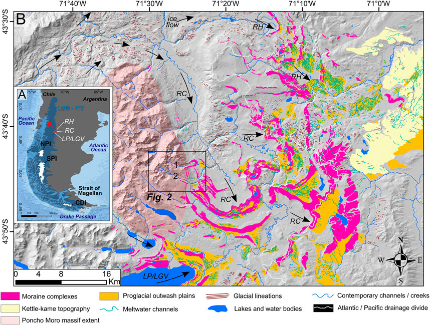
FIGURE 1. Location of study area. (A) Approximate former extent of the Patagonian Ice Sheet (PIS) during the Last Glacial Maximum (LGM), modified from Glasser et al. (2008) (dark blue polygon). Modern extents of the North Patagonian (NPI), South Patagonian Icefield (SPI), and Cordillera Darwin (CDI) Icefields are displayed in white. Bathymetric data from General Bathymetric Chart of the Oceans (GEBCO). Outlet glaciers that formerly occupied the study region are designated: RC: Río Corcovado, RH: Río Huemul, LP/LGV: Lago Palena/General Vintter glaciers. Spatial data are displayed in WGS84. (B) Shaded relief map (light azimuth: 315°, incline: 45°) based on the AW3D30 Digital Elevation Model (DEM) with overlaid glacial geomorphological data, adapted from Leger et al. (2020). Geomorphological data focus on the RC, RH and LP/LGV lateral and terminal glaciogenic deposits. The black box highlights the location of the El Loro (EL; 1) and Río Comisario (RCO; 2) valleys (Figure 2). Black arrows denote former ice-flow direction. The light red, transparent polygon highlights the geographical extent of the Poncho Moro massif. Spatial data are displayed in WGS84 and projected to UTM zone 19S.

2 Study Location

This study focuses on the mountain valleys and land-terminating palaeo-glaciers of the Poncho Moro massif, which is located on the eastern edge of the northern Patagonian Andes (Figure 1). The Poncho Moro massif today is characterised by maximum summit elevations of ∼2,100 m a.s.l., and is mostly ice-free, with the exception of one small glacier (∼0.1 km²) perched in the El Loro upper catchment (Figures 2, 3A). The current climate is classified as cool-temperate, due to the combined effects of the Peru-Chile current offshore from the Chilean Pacific coast and the SWW (Denton et al., 1999; Kaiser et al., 2007). However, due to the strong zonal orographic effect of the Patagonian Andes, total annual precipitation at the study site is reduced by ∼60% relative to the centre of the cordillera at ∼43°S. Consequently, the eastern valleys of the Poncho Moro massif are located at the western edge of the semi-arid Patagonian steppe climate zone (Garreaud et al., 2013; Fick and Hijmans, 2017). The massif is delineated to the north and east by the Río Corcovado valley, formerly host to a major topographically-controlled outlet glacier (Río Corcovado glacier) of the Patagonian Ice Sheet (PIS), which flowed eastwards from the ice-sheet divide during major Quaternary glaciations (Caldenius, 1932; Haller et al.,2003; Martínez et al., 2011; Leger et al., 2020). To the southeast of the Poncho Moro massif, the former Río Corcovado outlet glacier deposited a series of at least eight distinct moraine complexes (RC 0–VII) preserved across large expanses of the Argentinian foreland, five of which (RC III–VII) mark the local LGM and have been dated to marine isotope stage 2 (Leger et al., 2021). The Poncho Moro massif is therefore located towards the former eastern extremity of the PIS during the global LGM. Many valleys of the Poncho Moro massif display well-preserved sequences of lateral and terminal moraine complexes which enable the reconstruction of former mountain glacier extents (Leger et al., 2020, Figures 1, 2). We targeted two adjacent valleys for our investigation; the El Loro (EL) and Río Comisario (RCO) valleys (Figure 2), which are both oriented broadly northwest-southeast and were formerly host to western tributary glaciers of the Río Corcovado glacier. We chose these valleys because they both exhibit geomorphological evidence of glacier advances that locally cross-cut the RC III-VI margins, indicating younger moraine deposition occurred after the retreat of the Río Corcovado glacier from its LGM margins. These distinct lateral and terminal moraine complexes located near the EL and RCO valley mouths share similar distance-to-headwall properties (EL: 6.1 km; RCO: 7.1 km) (Figure 2). When reaching their respective outermost moraines, the former EL and RCO glaciers covered elevation ranges of between 2,100-890 m a.s.l. and 2050–1,100 m a.s.l., respectively.

FIGURE 2

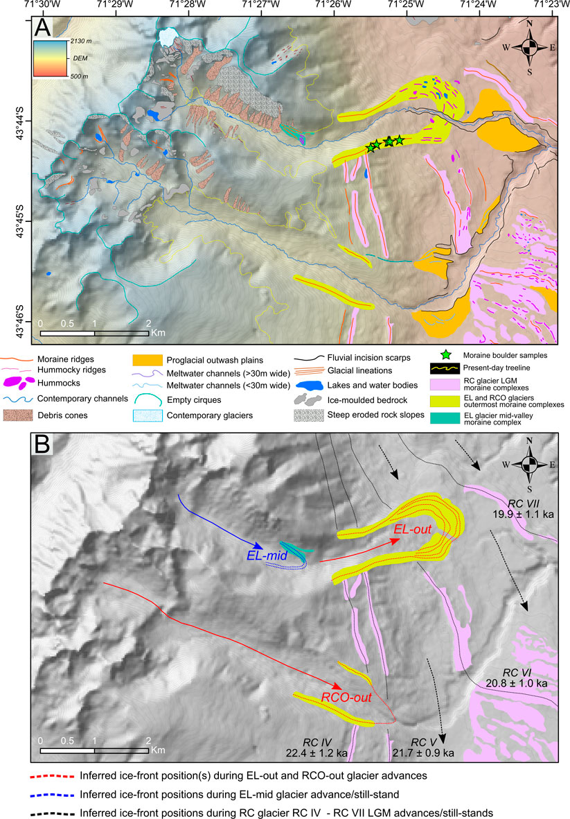
FIGURE 2. Geomorphological map of the EL and RCO valleys, northeastern Patagonia (see location in wider context, Figure 1). (A) DEM hillshade (AW3D30 DEM, light azimuth: 315°, incline: 45°) and geomorphological map of the EL and RCO valleys. Locations of moraine boulders sampled for TCN dating are indicated by green star symbols. The variable colouring of moraine complexes (pink/yellow/green) highlights the stratigraphic order of distinct palaeo-glacier advances/stillstands according to our geomorphological interpretations. (B) DEM hillshade, inferred moraine-complex stratigraphic relationships and former ice-flow directions of the Río Corcovado outlet glacier LGM advances/still-stands (black arrows), EL-mid advance/still-stand (blue arrow), EL-out and RCO-out advances (red arrows). The ages of the Río Corcovado LGM advances/still-stands are arithmetic mean ± 1σ standard deviations of moraine boulder exposure age populations reported by Leger et al. (2021) following Bayesian age model correction. Spatial data are displayed in WGS84 and projected to UTM zone 19S.

FIGURE 3

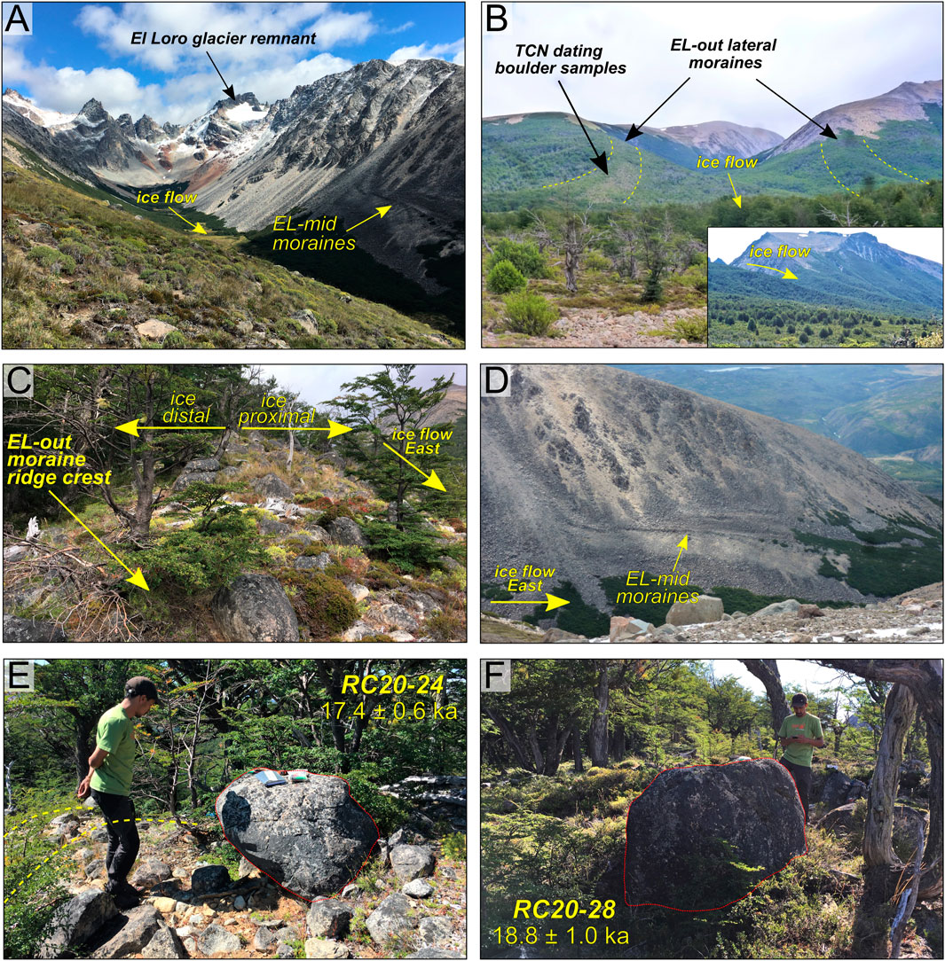
FIGURE 3. Field photographs of the EL valley, moraines and sampled boulders. (A) Northwest-facing photograph of the EL valley and its upper catchment displaying the EL-mid moraine ridges nested on the northern valley side. (B) Westward view of the EL valley mouth from the provincial road 44 (RP44). The EL-out lateral northern and southern (targeted for sampling) moraine ridges are highlighted by yellow dashed lines. The inset panel provides another, northward view of the same features from further afield. (C) Westward-facing photograph captured from the EL-out southern lateral moraine crest (targeted for sampling), ilustrating moraine crest sharpness, ice-proximal and ice-distal moraine-slope angles, moraine-surface boulder sizes, rough lithologies and concentration. (D) Northward view of the portion of the northern EL valley side displaying the preserved EL-mid moraine ridges. (E) South-facing photograph of an erratic granite boulder (sample RC20-24, highlighted by red line) deposited on the crest of the EL-out southern lateral moraine ridge and sampled for TCN dating. The curvature of the moraine crest is highlighted by yellow dashed lines (F) West-facing photograph of an erratic granite boulder (sample RC20-28, highlighted by red line) sampled for TCN dating.

The Poncho Moro massif surface geology is characterised by numerous lithologies including volcanic extrusives and sedimentary assemblages, and the EL and RCO catchments are dominated by the mid-cretaceous Río Hielo formation of granites with vein and dyke intrusions (Haller et al., 2003). Moraine boulders located on the outermost EL moraines are almost exclusively granitic and quartz-abundant, making these moraine deposits suitable for ¹⁰Be terrestrial cosmogenic nuclide (TCN) dating (Figure 3C,E,F).

3 Materials and Methods

3.1 Geomorphological Mapping

Major landforms and topographic features were initially identified using the freely available ALOS WORLD 3D - 30 m resolution (AW3D30: Japan Aerospace Exploration Agency) Digital Elevation Model (DEM). All mapped landforms were manually digitised in the WGS84 reference coordinate system projected to UTM zone 19S using the ESRI^TM World Imagery layer, characterized by ∼1.0 m resolution images from DigitalGlobe (GeoEye, IKONOS, 2000–2011) at the study site. In areas with dense vegetation and/or cloud cover, we undertook different colour-rendering comparisons using 10 m resolution Sentinel 2A true colour (TCI) and false colour (bands 8,4,3) products (available from https://scihub.copernicus.eu/). Detailed geomorphological mapping criteria along with the complete geomorphological map of the area are presented by Leger et al. (2020). Field-based mapping, ground-truthing and corrections of preliminary landform interpretations in the EL valley were conducted during the austral summer of 2020.

3.2 ¹⁰Be Terrestrial Cosmogenic Nuclide Dating

3.2.1 Dating Approach and Sampling

To establish the timing of local mountain glacier re-advances following initial PIS retreat, we targeted the outermost EL lateral moraines (Figures 2, 3), and sampled moraine boulders for ¹⁰Be surface exposure dating (e.g. Gosse and Phillips, 2001; Hein et al., 2010; Heyman et al., 2011). The selected granodiorite boulders (60–90 cm in height) resting directly on the moraine crest exhibited glacial polish and, in some cases, preserved striations, indicating minimal post-depositional surface erosion (e.g., Figure 3E,F). 1–2 kg samples were collected by hammer, chisel and angle grinder from the central section of the upper-most boulder surface, to a depth of 2–5 cm. Six boulders were sampled along a single continuous lateral moraine ridge (Table 1; Figures 2, 3). Collecting this number of samples from one landform aims to reduce potential uncertainties resulting from geological scatter and post-depositional processes (Putkonen and Swanson, 2003; Applegate et al., 2010; Heyman et al., 2011). Exposure ages were interpreted as dating moraine stabilisation following ice-front retreat and/or glacier tongue thinning, hence providing a minimum age for the glacier advance.

TABLE 1

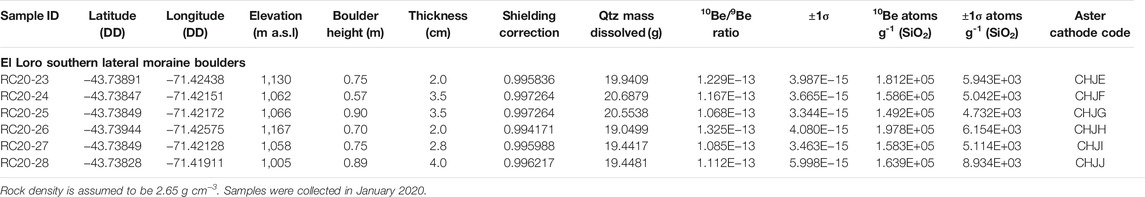
TABLE 1. Sample details and nuclide concentrations.

3.2.2 Sample Preparation, Wet Chemistry and Exposure-age Calculations

Samples were prepared at two cosmogenic nuclide laboratories: 1) the University of Edinburgh’s Cosmogenic Nuclide Laboratory for sample crushing/sieving and quartz purification/isolation; and 2) the National laboratory for Cosmogenic Nuclides (LN₂C) of CEREGE, Aix-en-Provence, France for post-purification wet chemistry. All ¹⁰Be/⁹Be ratios were measured by accelerator mass spectrometry at ASTER-CEREGE.

The samples were crushed in their entirety and sieved to isolate the 250–500 μm grain-size fractions. One to three treatments in HCl and H₂SiF₆ on a shaker table, which lasted up to 7 days per treatment, was performed to remove as much non-quartz minerals as possible (Bourlès, 1988). Pure quartz was obtained by repeated etching in a 2% HF and 1% HNO₃ solution for 24 h in a heated ultrasonic bath, with a sample to acid ratio of about 12 g L⁻¹. At least three etches were subsequently performed to remove atmospheric ¹⁰Be. The purified quartz samples were dissolved in concentrated HF and each sample, as well as one process blank, were spiked with between 0.42 and 0.46 mg of ⁹Be, in the form of an in-house carrier solution made from phenakite. After dissolution, the HF was evaporated off, and the solid residue was dissolved in HCl (10.2 mol L⁻¹), followed by Be(OH)₂ precipitation at pH ∼9 through the addition of NH₃ and re-dissolution in HCl. The solutions were first passed through anion exchange chromatography columns to remove Fe, Ti and Mn. After another evaporation and Be(OH)₂ precipitation step, HCl of lower concentration (1 mol L⁻¹) was added to dissolve the Be prior to passing the solution through cation exchange chromatography columns to isolate Be from B and Al. The Be fractions were then precipitated again as hydroxides and oxidised at ∼700°C. The resulting BeO samples were mixed with Nb powder and pressed into nickel cathodes for AMS measurements. Measurements are based on the in-house standard STD-11 with a ¹⁰Be/⁹Be ratio of (1.191 ± 0.013) 10⁻¹¹ (Braucher et al., 2015) and a ¹⁰Be half-life of (1.387 ± 0.0012) 10⁶ years (Chmeleff et al., 2010; Korschinek et al., 2010). Analytical uncertainties include ASTER counting statistics and stability (∼5%; Arnold et al., 2010) and machine blank correction. Process blank corrections ranged between 0.83 and 1.01% of calculated sample ¹⁰Be atoms.

Exposure ages were calculated using the online calculator formerly known as the CRONUS-Earth online calculator version 3 (Balco et al., 2008) with the ¹⁰Be Patagonian production rate of 3.71 ± 0.11 atoms g⁻¹ (SiO₂) yr⁻¹ (original value: Kaplan et al., 2007) obtained and re-calculated from the ICE-D online database (http://calibration.ice-d.org/). In this study, exposure ages were calculated using the time-dependent LSDn scaling scheme of Lifton et al. (2014) with 1σ analytical uncertainties. These ages assume no boulder surface erosion post-deposition and present no correction for shielding by snow, soil, or vegetation, following the rationale described in detail by Leger et al., 2021.

3.3 GIA-Related Uplift Estimates

The former PIS covered much of the study area during several Quaternary glaciations, resulting in glacial isostatic adjustment (GIA) of the land surface (Davies et al., 2020). Modern GPS station data from the region (Nevada Geodetic Laboratory data¹) report uplift rates of less than 1 mm yr⁻¹. If assumed to be constant through the period of exposure, such uplift rates would have an insignificant impact on ¹⁰Be production rates and numerical modelling outputs. However, the study area is located at the eastern limit of the Patagonian Andes and a significant amount of GIA-related surface uplift is expected to have occurred there during the Last Glacial–Holocene transition. Ice-sheet-wide glacial geomorphological mapping and palaeo-glacial reconstructions (Glasser et al., 2008; Davies et al., 2020) suggest that the PIS was ∼240 km wide at around 43°S during the local LGM, while data from the PaleoMIST global ice-sheet reconstruction dataset (Gowan et al., 2021) estimate that maximum PIS thickness during the global LGM reached approximately 1,650 m at these latitudes. In this region of Patagonia, the majority of the ice mass is thought to have melted between 19 and 15–16 ka (Moreno et al., 2015; Leger et al., 2021), with crustal unloading leading to GIA and to significant surface uplift. To estimate the effect of local GIA on ¹⁰Be production and palaeo-climate outputs from glacial numerical modelling, we evaluated former time-varying isostatic uplift and subsidence rates using the ∼5 km resolution PaleoMIST global ice-sheet reconstruction dataset (ice-thickness data: Gowan et al., 2021) and the gFlex lithospheric flexure model (Wickert, 2015). We calculated the GIA signal for three spatially-invariant lithospheric elastic thickness values (30, 35 and 40 km; after Lange et al., 2014). As estimates of local mantle viscosity (Ivins and James, 2004; Lange et al., 2014) indicate isostatic response timescales shorter than PaleoMIST’s 2.5-kyr temporal resolution, we consider isostatic adjustment to be fully completed within each time step. With this analysis, we produced a paleo-elevation change time series and corrected palaeo-topography at the study site from 25 ka to present.

3.4 Numerical Modelling of the EL and RCO Palaeo-Glaciers

In order to investigate the interaction between climate and the dynamics of the former EL and RCO glaciers, we employed a spatially-distributed ice-flow model, coupled with a positive degree-day (PDD) surface mass balance (SMB) parameterisation. Model parameters were tuned to fit best the simulated ice extent with the observed geomorphological moraine record. Similar models have been used elsewhere to investigate glacier response to climate change (e.g., Adhikari and Marshall, 2012; Jouvet and Funk, 2014; Wijngaard et al., 2019). The ice-flow model used here follows standard equations of the Shallow Ice Approximation (SIA; Hutter, 1983). While this approximation does not resolve all of the terms of the nonlinear glacial stress balance (i.e., longitudinal and transverse stresses), it is much faster to run than higher-order or Stokes models, allowing for ensembles of multi-century simulations exploring a comprehensive range of SMB and ice-dynamical parameters (see below). Other studies have shown this to be an appropriate approximation for modelling small mountain glaciers with small aspect ratios (Wijngaard et al., 2019). We implemented the model over a ∼30-m resolution topographic grid derived from the AW3D30 DEM.

3.4.1 Ice Flux

In our model, ice flux was calculated recurrently at a given time-step interval, set to 0.1 years, for each ∼900 m² grid cell, and accounted for both internal deformation and basal sliding. Internal deformation is controlled by the interaction of the glacier’s surface slope and combined weight. In this study we used a uniform ice density value of 916.7 kg m⁻³. Ice flow occurs when basal shear stress (τ), defined by Glen’s flow law (Eq. 1), exceeds a given yield stress value (Cuffey and Paterson, 2010):

$\epsilon =A{\tau }^n(1)$

where ε is the horizontal shear strain, τ is basal shear stress (Pa) and n and A are constants representing the combined rheological impacts of ice temperature and ice crystal orientation. n and A were here set to values of 3.0 and 1.0 × 10⁻¹⁶ Pa⁻³ yr⁻¹ (Hubbard et al., 2005), respectively. Such values are commonly used to account for irregularities in glacier-ice structure such as crevasse fields, meltwater pockets and other impurities (Cuffey and Paterson, 2010).

As geomorphological evidence of subglacial lineations and ice-moulded bedrock outcrops suggests the EL and RCO glaciers were at least partly warm-based, modelled ice flux therefore also needed to incorporate basal sliding, which is defined by Eq. 2 based on Weertman’s law (Weertman, 1957):

$u_s=A_s{{\tau }_d}^{\rho }(2)$

where $u_s$ is basal sliding velocity (m yr⁻¹), A_s and $\rho$ are constants, and τ_d (Pa) is a given value for driving stress. In this study, $\rho$ = 3, which is within the range observed in laboratory and field-based investigations (Budd et al., 1979; Bindschadler, 1983). Based on empirical measurements of sliding velocity obtained for similarly-sized, mid-latitude temperate mountain glaciers (e.g., Engelhardt et al., 1978; Blake et al., 1994; Cohen et al., 2000), we use a uniform value of 5.0 × 10⁻¹⁵ Pa^−1/3 m yr⁻¹ for A_s, which yields a sliding rate of 5.0 m yr⁻¹ where driving stress (τ_d) is 1 bar. For the EL-outermost advance reconstruction, this parameterisation of basal sliding increased the mean glacier surface velocity by ∼6.2 m yr⁻¹ relative to simulations implementing no basal sliding. Such a contribution represents ∼18% of mean steady-state glacier surface velocity; a ratio that is close to those reported by empirical measurements of sliding speed versus surface speed of glaciers sharing similar properties (e.g., Cohen et al., 2000; 16%). However, it is important to note that estimating a meaningful value for basal sliding velocity is amongst the most challenging and uncertain components of modelling warm-based glaciers (Cohen et al., 2005). Moreover, asuming that the modelled glaciers were warm-based across their entire area and not polythermal is subject to debate and yields uncertainties further addressed in the discussion section of this paper.

3.4.2 Surface Mass Balance

Modelled ice thickness for a given grid cell controls the modelled glacier profile and is defined by the sum of ice flux and SMB. Here we parameterised SMB (b: m w.e.) using a PDD model, defined, at a given elevation (z), by Eqs 3–5:

$b=Pr-\left(PDD\right)T, T>0(3)$

$b=Pr, T<0(4)$

$T=zELA\frac{\gamma }{1000}+TSL(5)$

where Pr is precipitation (m ice yr⁻¹), PDD is the positive degree-day melt factor (m ice °C⁻¹ yr⁻¹), and γ is an adiabatic lapse rate (ALR; °C km⁻¹), which enables interpolating atmospheric temperature T (°C) at an elevation z (m a.s.l.) using a given value for temperature at sea level (TSL: °C). We use an ALR of 6.5°C km⁻¹ (e.g., Wallace and Hobbs, 2006; Roe and O’Neal., 2009). As shown by the above equations, PDD only causes surface melt when atmospheric temperature exceeds 0°C (Figure 4). A constant precipitation rate is applied and normally distributed across the domain (e.g., Roe and O’Neal, 2009; Roe, 2011), thus assuming little geographical and altitudinal variation across the relatively small EL and RCO valley catchments (∼7.5 and ∼10.3 km², respectively). This simple SMB model does not independently consider ablation caused by sublimation or ice-front breakoff, nor does it take into account other sources of accumulation such as avalanches. It also neglects the percolation and refreezing of meltwater and assumes that all melting ends up as runoff (after Roe and O’Neal, 2009).

FIGURE 4

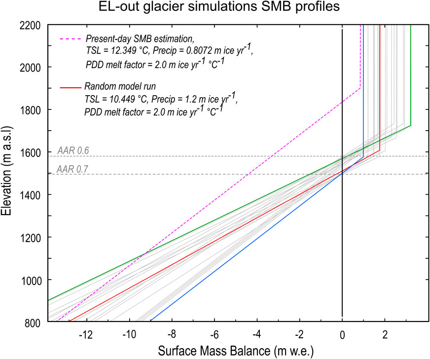
FIGURE 4. A sample (n = 20) of Surface Mass Balance (SMB) profiles (grey and coloured lines) of the EL-out ice-flow model simulations using a positive degree-day SMB parameterisation. The pink dashed line is a surface mass balance profile representative of our modern-day climate estimation, according to our assessment of modern local atmospheric temperature and precipitation (section Modern Climate), when using a PDD value of 5 mm w.e. d⁻¹°C⁻¹. Note that the SMB profiles for EL-out model runs intersect the 0 SMB value (i.e., the glacier equilibrium line) at elevations associated with AAR values of between 0.6 (green line) and 0.7 (blue line), which are used as threshold values to constrain our model simulations.

3.4.3 Modern Climate

Investigating former climate change from palaeo-glacier SMB requires the determination of base values for precipitation and temperature that are representative of average modern local climate. Mean annual temperature data were acquired from five different weather stations located in the towns of Corcovado (n = 1, 43°54′S; 71°46′W), Trevelin (n = 3, 43°5′S; 71°27′W) and Río Pico (n = 1, 44°10′S; 71°22′W). These data were obtained from the Argentinian National Agricultural Technology Institute (www.argentina.gob.ar/inta). TSL values were extrapolated from mean annual temperatures using an ALR of 6.5°C km⁻¹, for the years between 1982 and 2015 (depending on the weather station). The values ranged between 12.06 and 12.65°C. Given these data, a mean TSL value of 12.35°C was here considered representative of modern regional atmospheric mean annual temperature. Using a 6.5°C km⁻¹ ALR, this is equivalent to a mean annual 0°C isotherm elevation of 1900 m a.s.l. As measured precipitation data was unavailable, local modern precipitation was obtained from the 1-km spatial resolution global-land WorldClim 2 dataset (WC2; Fick and Hijmans., 2017), which spatially interpolates available weather station data and provides monthly climate data averaged over 1970–2000. From this dataset, modern-time total annual precipitation was averaged over the simulated steady-state surface area of the EL (16 data points) and RCO (19 data points) palaeo-glaciers to derive estimates of 740 mm w.e. and 722 mm w.e., respectively. Using an ice density of 916.7 kg m⁻³, and assuming that all precipitation is accumulated as ice, these values are equivalent to 0.8072 and 0.7876 m³ ice m⁻² yr⁻¹ of accumulation, respectively. Consequently, for each simulation, we calculated precipitation and temperature variations relative to modern-day base values of Pr_EL = 0.8072 m ice yr⁻¹, Pr_RCO = 0.7876 m ice yr⁻¹, TSL = 12.35°C.

3.4.4 Model Simulations

The model was used to simulate two distinct former advances/still-stands of the EL palaeo-glacier (EL-out and EL-mid) and one advance of the RCO palaeo-glacier (RCO-out), each relating to well-defined moraine complexes observed in the field (Figures 2, 3). Model simulations were constrained by PDD melt factor thresholds of 5.0 and 9.0 mm w.e. d⁻¹°C⁻¹, consistent with values reported from stack measurements on mid-latitude mountain glaciers from different regions of the world (Braithwaite and Zhang, 2000; Hock, 2003). This is also consistent with PDD melt factors measured on Patagonian glaciers, which typically range from 5.0 to 7.5 mm w.e. d⁻¹°C⁻¹ (De Angelis, 2014). Accumulation area ratios (AAR) of 0.6 and 0.7 were also implemented as additional constraints for our simulations. Such values are based on worldwide observations that AARs >0.7 or <0.6 have produced less realistic SMB profiles for debris-free, mid-latitude temperate mountain glaciers in a state of mass-balance equilibrium, and >4 km² in surface area (Benn et al., 2005; Kern & László, 2010; Pellitero et al., 2015). However, this assumption yields significant uncertainties as it is challenging to estimate former glacier debris cover evolution, which, if sufficiently thick, could substantially lower the AAR through glacial surface insulation (Osmaston, 2005). Moreover, surface debris cover is likely to fluctuate through time as glacier retreat and thinning causes valley-side destabilisation. The AAR was calculated for each simulated ice extent deemed to match the sampled moraines using model-output ice-thickness raster data and the SurfaceVolume_3D ArcGIS tool (following Pellitero et al., 2015). Ice-front to moraine fit was assessed by producing modelled ice-surface longitudinal cross-section profiles along the glacier centre flowline for each simulation and comparing ice-front location with terminal moraines. ArcGIS 10.8 software was subsequently employed to digitize ELA polylines and total glacier and accumulation zone polygons using ice-surface topographic contour lines, prior to computing AARs using polygon 3D surface areas. Therefore, within such PDD melt factor and AAR constraints, a minimum of thirty to forty simulations were adjusted for each of the EL and RCO glaciers and for each reconstructed glacier-front position (EL = 2 positions, RCO = 1 position) to determine ranges of ideal precipitation and temperature parameter combinations producing moraine-matching glacier extents. In total, near one hundred multi-century model simulations with differing SMB parameters were adjusted to fit the geomorphological record, excluding model sensitivity test runs (see Model Sensitivity Test section below) and multi-century simulations that correlated poorly with observed moraine locations. For each given round-number PDD melt factor (5–9), a second order polynomial regression equation with a R² value greater than 0.99 was calculated to provide a relationship between ideal precipitation and temperature parameter combinations.

In contrast to Stokes or high-order numerical glacier models, our model does not require high computational speeds and enables comparing numerous simulations against the geomorphological record using a wide range of SMB parameter values. It also enables palaeo-temperature and palaeo-precipitation estimations even in the absence of a modern active glacier at the study site, although the lack of studied modern glaciers in the Poncho Moro massif makes calibrating the model against present-day glaciological and meteorological conditions challenging, leading to larger uncertainties in SMB parameter range estimates. Unlike palaeo-climate estimations relying on ΔELA comparisons (e.g., Sagredo et al., 2018; Sun et al., 2020), our method does not require a modern ELA value to derive palaeo-temperature estimates. Furthermore, it does not assume that precipitation was identical to the present at the time of the reconstructed glacier advance/still-stand, because accumulation is already taken into account in our SMB parameterisation. We thus consider SMB model outputs as more realistic palaeo-climate indicators and chose not to compare our results with an estimated modern ELA, as in the absence of active glaciers in the study area, this would be highly subjective.

3.4.5 Model Sensitivity Tests

In order to test confidence in using our SMB parameter combinations as potential palaeo-climate indicators, we tested the model by running simulations with different ice softness parameters (constant A in Glen’s flow law; Eq. 1) to simulate different ice-temperature regimes. While the default value chosen is 1.0 × 10⁻¹⁶ Pa⁻³ yr⁻¹, which corresponds approximately to a mean glacier-ice temperature of −2°C, we also conducted model runs with boundary values of 0.5 × 10⁻¹⁶ and 1.5 × 10⁻¹⁶ Pa⁻³ yr⁻¹, corresponding to ice temperatures of approximately −5 and 0°C (Cuffey and Paterson, 2010), respectively (Table 2). The results generated a maximum glacier volume increase (A = 0.5 × 10⁻¹⁶) of 16% and a maximum decrease (A = 1.5 × 10⁻¹⁶) of 7%. Such fluctuations in ice thickness are mostly confined to the accumulation zone of the glacier, and therefore they have minimal impact on the extent and thickness of the glacier tongue. The greatest change observed in glacier-front location as a result of sensitivity to fluctuations in A values was a retreat of 94 m, which represents a 2.5% decrease in glacier extent. For most other simulations, maximum glacier extent remained within a 1% fluctuation to the original (A = 1.0 × 10⁻¹⁶). Therefore, modifying the glacier-ice temperature regime within a −5–0°C range has little impact on the model’s ability to match the geomorphological moraine record.

TABLE 2

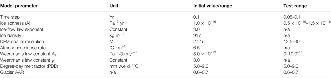
TABLE 2. Coupled ice-flow and positive degree-day SMB model input parameters.

Note that our adjustment of the ice-softness parameter is equivalent to the consideration of a correction factor in Wijngaard et al. (2019) -- i.e., a factor meant to represent the inaccuracies inherent in the SIA. In this sense, the low sensitivity to Glen’s flow constant suggests a wide range of correction factors, or equivalently that the assumptions of the SIA have a relatively small impact on steady glacier geometry and length.

We also conducted test model runs by removing the effect of basal sliding (Table 2). The results showed that although the glacier took up to 30 years longer to build up, steady-state glacier extent and thickness were identical to runs conducted with basal sliding, indicating that changing the basal sliding velocity within a realistic range had little impact on steady-state ice thickness, ice-front location and glacier surface profile. However, we do note that doubling of the baseline sliding parameter described in Ice flux section caused a noticeable reduction in simulated ice-thickness and augmentation in ice-front extent.

We also tested the model’s sensitivity to DEM spatial resolution by running a series of simulations using the ALOS PALSAR DEM product (Dataset²) which, in the studied region, uses radiometric terrain correction to re-sample the AW3D30 DEM product to 12.5 m spatial resolution. Despite a 2.4 times greater spatial resolution, the simulated ice thickness, glacier extent, surface velocity and years required to reach steady-volume were all identical to simulations conducted using a ∼30 m spatial resolution DEM.

To compare our model outputs to the more commonly-used method of land-terminating glacier surface reconstruction using a simple flowline model (e.g., Huss et al., 2007; Banerjee and Shankar, 2013), we conducted simulations using GlaRe (Pellitero et al., 2016) and included the associated methodology and results in the Supplementary Material.

To assess variability in PDD melt factor values from different palaeo-glaciers of the region, and to obtain further local climatic constraints during the late-glacial period, we compared SMB parameters required for moraine-matching simulation of both the EL and RCO glaciers. We considered it reasonable to assume that climatic conditions are and were likely very similar between the two adjacent valleys. This is supported by WC2 total annual precipitation data, indicating a 1970–2000 mean of 722 mm w.e. over the simulated RCO glacier surface area (Fick and Hijmans., 2017), representing a 2.4% decrease relative to the adjacent EL valley (740 mm w.e.). Using identical AAR and PDD melt factor constraints for the SMB model as for the EL glacier simulations, we adjusted thirty model runs with a simulated ice-front extent that matches the RCO valley moraine system in order to analyse input SMB parameter combinations required. Assuming that this advance was contemporaneous with the EL late-glacial advance sampled for TCN dating, analysing the overlap in the resulting climate constraints from the two sets of simulations can provide better confidence in resulting temperature and precipitation ranges required for moraine-matching simulations, and enables assessment of surface melt-rate variability between the two glaciers. Indeed, it is feasible and has been observed in other modern glaciated massifs (e.g., Glacier d’Arsine and Glacier Blanc, Ecrins massif, France; Vivian, 1967; Vivian and Volle, 1967), that two proximal mountain glaciers with similar elevation ranges and climatic conditions can display substantially different surface debris covers, mainly as a result of contrasting susceptibility of upper catchment slopes to rockfall and rock-slope failures (Benn et al., 2003). Therefore, some variability in former surface melt rates between the two glaciers may be expected, which may hinder the quality of overlaps in SMB parameter ranges required for the moraine-matching simulations of both glacier advances, in the hypothetical case of these advances being triggered by the same climatic event.

4 Results

4.1 Geomorphology

4.1.1 Valley Geomorphology

In the upper EL and RCO catchments, above the treeline (1,400–1,500 m a.s.l.), the valley floors are characterised by thick glacial debris cover and patterned ground displaying polygonal structures that are characteristic of periglacial environments and indicative of cryoturbation and frost heaving following ice retreat. These debris accumulations are interspersed in the steeper portions of the valley bottom by outcrops of ice-moulded and striated bedrock (Figure 2A). The upper EL and RCO catchments contain numerous empty cirques, while the EL valley still features one glacier remnant (∼0.05 km²) perched below its highest summit (∼2095 m a.s.l.; Figure 2A). Debris cones and rock talus mantle the steep valley sides and indicate frost shattering of cliffs and local catchment ridges. Consequently, substantial volumes of rockfall debris partly obscure the palaeo-glacier bed topography.

4.1.2 Glacial Moraines

Geomorphological mapping from field and remotely-sensed observations reveals the preservation of three distinct moraine complexes deposited by glacier-ice confined within the EL valley, two of which are also present in the RCO valley (Figure 2).

In the EL valley, the outermost set of moraine ridges (EL-out) is located towards the eastern edge of the Poncho Moro massif, 1.5–2 km to the east of the valley mouth, and indicates a northeastward advance of the EL glacier. This complex can be linked to well-defined, ∼1.5 km long, single-crested and prominent (30–35 m above the valley floor) lateral moraines preserved on both valley flanks (mean crest-surface slope: 13°; Figure 3). Both of these lateral ridges bifurcate downstream into a series of cross-valley arcuate ridges and hummocks spreading at least 1 km across a gently-sloping surface, which is suggestive of numerous episodes of terminus extent fluctuation and/or re-advances of the EL glacier (Figure 2A). The geometry of these terminal ridges and mounds suggest a piedmont-style former EL glacier terminus. The lateral moraine complex cross-cuts at right angles the RC III-VI moraines previously deposited by the Río Corcovado outlet glacier (Figure 2). Consequently, the advance of the EL glacier must post-date the RC VI moraine, which has been dated using ¹⁰Be TCN dating to 20.7 ± 1.0 ka (Leger et al., 2021). Moreover, directly downstream of the terminal moraines, a broad (0.85 km² in area) low-gradient (2°) and homogeneous surface composed of fluvial sand and gravel progrades eastwards (43°43′59″S; 71°23′53″W). This terrace deposit, which was incised by the EL river post-deposition (∼10–15 m incision), is interpreted as a proglacial outwash plain. It thus provides further evidence of a former glacier margin stabilised directly upstream from its location. The location of this deposit indicates that former proglacial rivers were constrained towards the north by the previously-deposited RC VII moraine. Such stratigraphic relationship further suggest that the EL-out advance is younger or similar-in-age to the deposition of the RC VII moraine, previously dated to 19.9 ± 1.1 ka (Leger et al., 2021). We targeted the prominent, sharp-crested southern lateral moraine ridge for TCN dating based on the assumption that it highlights maximum palaeo-glacier thickness and thus the most extensive, morphostratigraphically-oldest advance of the EL glacier into this moraine complex.

The RCO valley contains an analogous set of single-crested and prominent lateral moraine ridges nested on both valley flanks, which are located towards the mouth of the valley (Figure 2). These moraines exhibit curved geometries towards their distal ends, enabling a rough extrapolation of the former ice-front position during this advance. However, the exact position of the terminal moraine is uncertain as a consequence of local erosion by post-retreat fluvial incision. This moraine complex and associated advance are termed RCO-out and we consider it morphostratigraphically-equivalent to the EL-out moraine complex.

A second, younger complex of latero-terminal moraine ridges are evident in the EL valley, located approximately 3.8 km from the valley headwall. These moraines demarcate a former glacier front positioned ∼2.4 km upstream (∼40% glacier-extent decrease) from the EL-out margins. This younger complex is composed of three adjacent ridges that extend for ∼500 m, are curved towards their distal ends, and reach an elevation of ∼1,300 m a.s.l. The ridges are relatively low in relief (2–5 m), with less well defined crests, and are only discernible on the northern valley flank (Figure 3A,D). Their proximal end seems to have been buried by the post-glacial accretion of rock talus. Their geomorphology is suggestive of a significantly lower sediment volume delivery and/or ice-front residence time than the EL-out moraine sequence. We refer to these deposits as the EL-mid moraine complex and associated glacier advance/still-stand. We did not identify geomorphic evidence of a similar mid-valley moraine complex in the RCO valley.

Finally, in both the EL and RCO valleys, smaller moraine ridges can be discerned in the upper catchment limits, near the downstream edge of isolated eastward-facing (down-wind) cirques, nested at elevations of between 1,500 and 1800 m a.s.l. (Figure 2). We only observed a single set of these moraines in the EL valley while the RCO catchment displays at least four cirques where such ridges are preserved. They highlight the former stabilisation/re-advance of small glaciers nested on the catchment’s highest, wind-sheltered slopes. We hypothesise these deposits to be relatively young, perhaps late-Holocene or Neoglacial in age, given the late-Holocene relative glacier-extent loss observed in other Patagonian mountain valleys (e.g. Nimick et al., 2016; Reynhout et al., 2019).

4.2 ¹⁰Be Surface Exposure Ages

The six boulders from the southern lateral moraine of the EL valley range in age from 16.4 ± 0.5 to 19.5 ± 0.6 ka and yield an arithmetic mean exposure age of 18.0 ± 1.15 ka. The age population demonstrates a relatively high and >1 mean square weighted deviation (MSWD) value of 3.78, thus suggestive of greater age scatter than can be predicted solely by 1σ analytical uncertainties (Table 3; Figure 5). Furthermore, the MSWD value exceeds the criterion k, which is dependent on the degree of freedom, and is equal to 2.26 given the number of samples (n = 6; Wendt and Carl, 1991; Jones et al., 2019a). Statistically, a MSWD > k suggests that the probability that the age population is representative of a single landform is <95% and thus the weighted mean cannot be used as an estimate of the average exposure age for the moraine (Jones et al., 2019a). Despite significant geological scatter, we do not identify obvious outliers as all ages fall within the population’s 2σ envelope (Figure 5).

TABLE 3

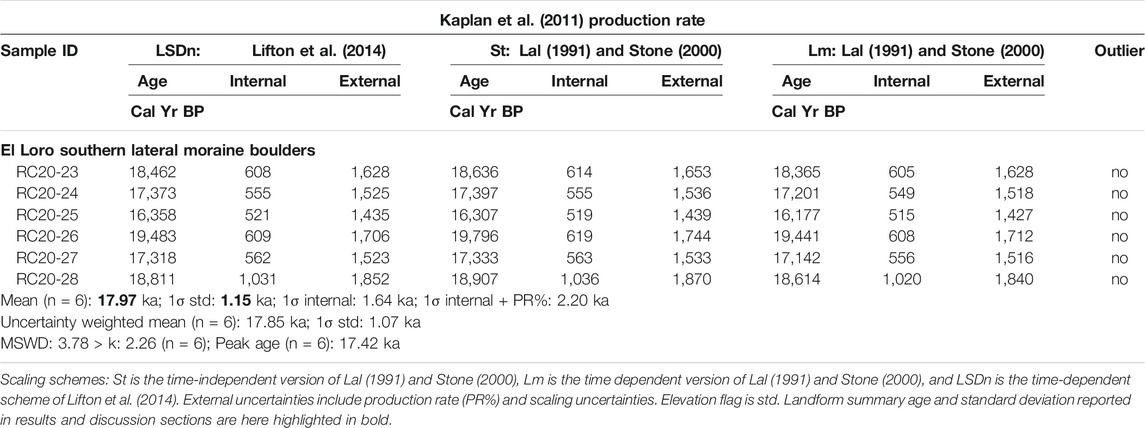
TABLE 3. Exposure ages and summary statistics.

FIGURE 5

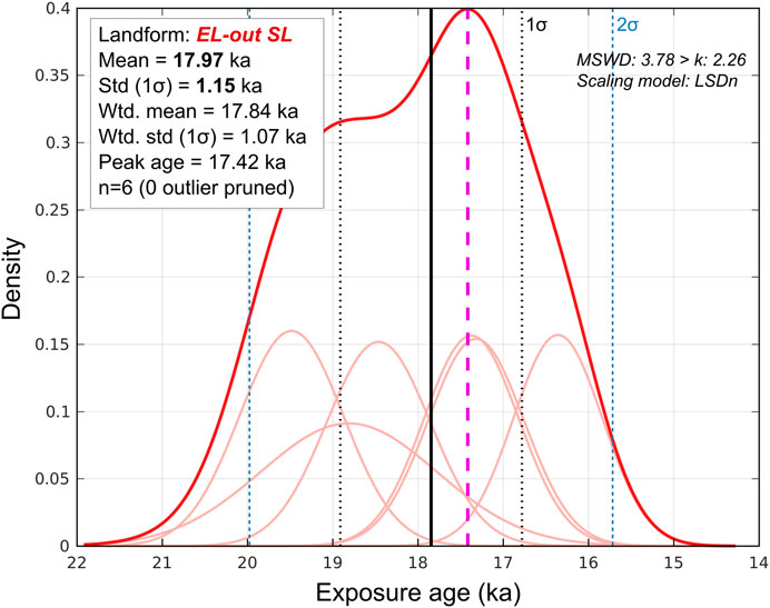
FIGURE 5. Kernel density plot, adapted from plots produced using the iceTEA tools for exposure dating (Jones et al., 2019a; http://ice-tea.org/en/) and TCN dating summary statistics for the EL-out southern lateral (EL-out SL) moraine boulder samples (n = 6). Thick red curve represents the summed probability distribution for the age population while thin red curves depict Gaussian curves for individual samples. Vertical black lines denote the arithmetic mean, while thin black and blue vertical dashed lines denote the 1 σ and 2 σ confidence intervals of the mean, respectively. Thick purple and dashed vertical line highlights the peak age associated with the summed probability distribution. Std: standard deviation, Wtd. mean: uncertainty-weighted mean, Wtd. std: uncertainty-weighted standard deviation.

4.3 GIA-Related Uplift

Output from the gFlex lithospheric flexure model (Wickert, 2015) suggests that the surface elevation of the study site at 20 ka was between 148 m (40 km elastic thickness) and 151 m (30 km elastic thickness) lower than modern elevations measured in the field (Table 4). These cumulative uplift values are close to the estimate of 113.9 m obtained from the global ICE-6G model (Peltier et al., 2015) and a three-layer approximation of the VM2 Earth model implemented in the IceTEA tools for exposure ages (Jones et al., 2019b). GIA-related uplift modelling using gFlex suggests that over 99% of post-LGT uplift occurred between 20 and 12.5 ka in response to local ice-sheet disintegration (Table 4). The 2.5 kyr temporal resolution of the PaleoMIST dataset (Gowan et al., 2021) provides local, time-varying GIA-related uplift rates approximating 9.1, 39.4 and 11.6 mm yr⁻¹ between 20–17.5, 17.5–15, and 15–12.5 ka, respectively. Using such uplift rates, a mean elastic thickness of 35 km, and a mean age of 18.0 ka for the EL-out advance based on our exposure age population, we estimate GIA to have caused approximately 131 m of surface uplift since the time of the EL-out glacier advance. The impact of such surface elevation change on former ¹⁰Be production rates and exposure ages is inferior or equivalent to 1σ analytical uncertainties (between 0.47 and 0.74 ka; <4% age corrections), and is thus not considered applicable here. However, the inferred mean uplift of 131 m since 18 ka, the approximate time of the EL-out glacier advance, requires taking into account 0.85°C of local atmospheric temperature adjustment when applying an ALR of 6.5°C km⁻¹. Consequently, we adjusted our modelling ELA and temperature outputs using 131 m of surface uplift and 0.85°C of relative temperature lowering for a given model simulation in order to account for GIA-related uplift since the time of the reconstructed advance. These reconstructed uplift rates are inherently subject to uncertainties associated in part with the assessment of parameters such as regional palaeo-ice thicknesses, lithospheric thickness and mantle viscosity (Peltier et al., 2015; Wickert, 2015; Gowan et al., 2021). However, our estimates are similar in magnitude to modern uplift rates observed for regions of Patagonia currently experiencing rapid isostatic uplift due to present-day glacial retreat and ice-sheet thinning. For instance, Lange et al. (2014) reported modern uplift rates from geodetic GNSS observations of up to 41 ± 3 mm yr⁻¹ near the centre of the South Patagonian Icefield (SPI), and of approximately 20 mm yr⁻¹ towards the margins of the SPI. Although regional tectonic uplift may also contribute a small part of this uplift (Richter et al., 2016), these modern rates suggest that our post-LGT GIA-uplift estimates are comparable and relatively realistic for Patagonia.

TABLE 4

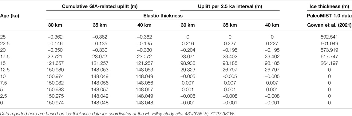
TABLE 4. gFlex GIA-related surface elevation and PaleoMIST ice-thickness data.

4.4 Numerical Modelling Results

4.4.1 Glacier Geometry

Our spatially-distributed ice-flow model generated simulated glacier surfaces that match lateral and terminal moraine complexes well for a given advance/still-stand. However, while steady-state simulated ice-fronts matched the terminal moraine record for the EL-mid and RCO-out simulations, the simulated EL-out ice front stabilised ∼100 m upstream from the moraine complex. Further ELA lowering did not generate significant ice-front advances, instead inducing a wider piedmont-style ice front overrunning the lateral moraine ridges. There are numerous possible reasons for such a misfit, including, for instance, the model’s inability to capture spatially-varying basal sliding conditions and ice temperature properties, and the possibility of post-advance debris accumulations near the former glacier terminus, which could have caused a decrease in basal slope gradient. Therefore, for the EL-out simulations, we based our moraine-fit quality assessment on the location of the ice margin relative to the prominent EL-out lateral moraine ridges. Simulated steady-state glacier volume for the EL-out glacier advance ranged between 0.614 km³ (0.563 Gt) and 0.769 km³ (0.705 Gt) depending on SMB parameter combinations, while steady-state surface area ranged between 7.154 and 7.234 km² (Table 5; Figures 6, 7). Simulations took between 100 and 170 years to reach steady volume from a no-ice initial state. Maximum ice thickness ranged between 272 and 315 m and glacier length along the central flowline approximated 6.1 km from the valley headwall. Mean steady-state glacier-surface velocity, which is positively correlated to accumulation rates and thereby ice flux, ranged between 31.9 m yr⁻¹ (run with lowest precipitation) and 61.0 m yr⁻¹ (run with highest precipitation) (Table 5; Figure 6). These surface velocities are consistent with average surface velocities measured in the field and through remote sensing of land-terminating and similarly-sized glaciers from northern Patagonia (Rivera et al., 2012) and other mid-latitude alpine massifs (e.g., New Zealand Southern Alps, Mont-Blanc massif; Millan et al., 2019). Corresponding glacier geometry statistics for the RCO-out and EL-mid advances/still-stands are compiled in Table 5.

TABLE 5

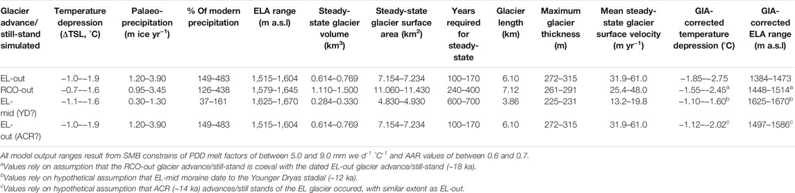
TABLE 5. Numerical model output statistics and ranges.

FIGURE 6

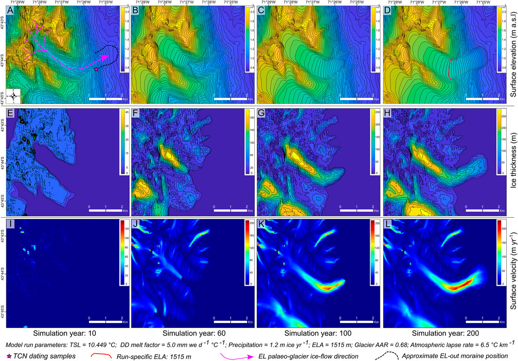
FIGURE 6. Ice-flow model output data (∼30 × ∼30 m grid-cell spatial resolution) for one selected model simulation of the EL-out advance. (A–D) Surface elevation data (m a.s.l.) including AW3D30 DEM data plus simulated ice thickness, (E–H) ice thickness data (m), and (I–L) ice-surface velocity data (m yr⁻¹); for simulation years 10 (panels A, E, I), 60 (panels B, F, J), 100 (panels C, G, K) and 200 (steady-state volume, panels D, H, L). Note that colorbar values and scaling are panel-specific. Equivalent figures specific to the RCO-out and EL-mid advances/still-stands model simulations can be found in the Supplementary Figures S1,2.

FIGURE 7

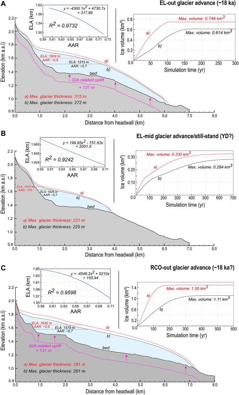
FIGURE 7. Elevation profile graphs (above present-day sea level) of bedrock topography (AW3D30 DEM data) and simulated steady-state ice thickness along the central glacier flowline for the EL-out (A), EL-mid (B) and RCO-out (C) simulations. The purple dashed lines denote the estimated former bed surface elevation at the time of the EL-out advance, prior to GIA-related uplift (131 m). For each profile graph, the two ice-surface profiles highlighting maximum and minimum simulated ice-thicknesses for a given advance/still-stand are represented. These two profiles also represent boundary AAR values (0.6 vs. 0.7). Each panel also features an ice-volume time series line graph for minimum and maximum ice-volume simulations, as well as a standard regression analysis establishing the best-fit second-degree polynomial relationship between ELAs (km a.s.l.) and AARs for all simulations of a given glacier reconstruction.

4.4.2 Palaeo-Temperature

For the EL-out glacier advance, here dated to 18.0 ± 1.15 ka, simulations constrained by PDD melt factor values ranging between 5.0 and 9.0 mm w.e. d⁻¹°C⁻¹ and by AAR values of between 0.6 and 0.7 required a range of temperature depression values relative to our present-day mean annual atmospheric temperature estimation (section Modern Climate) of between −1.0 and −1.9°C (Table 5; Figure 8A). Including correction for cumulative GIA-related surface uplift relative to today (−0.85°C; Table 4) causes temperature depression values to range between −1.85 and −2.75°C. Moraine-matching simulations conducted using a temperature depression that is greater than 2.75°C caused the ELA to increase and the glacier’s accumulation zone to expand so that the AAR becomes greater than 0.7, a ratio that is rare for a mid-latitude, land-terminating mountain valley glacier in a state of mass-balance equilibrium (Braithwaite and Müller, 1980; Kern and László, 2010), and is here assumed unlikely (Table 5; Figure 8A).

FIGURE 8

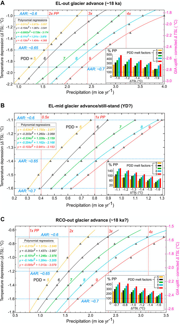
FIGURE 8. Ice-flow model temperature depression and precipitation parameter combinations for each moraine-matching simulation (grey triangles) of the EL-out advance (A), the EL-mid advance/still-stand (B) and the RCO-out advance (C), for a given round-number positive degree-day melt factor value between 5.0 and 9.0 mm w.e. d⁻¹°C⁻¹. Each graph displays colour-coded second-degree polynomial regression curves and equations for each round-number positive degree-day melt factor (n = 5). All regression equations are associated with R² values >0.99. Each diagram also display histograms indicating the % precipitation associated with each simulation relative to present precipitations (% PP) values, for a given temperature depression value and degree-day melt factor (colour-coded bars). The horizontal dashed line represents modern precipitation (100%). Note that GIA-corrected temperature depressions include the hypothetical assumptions that the EL-mid advance/still-stand dates to the YD (∼12 ka), and that the RCO-out advance is coeval with the EL-out advance (∼18 ka).

4.4.3 Palaeo-Precipitation

The model simulations required precipitation values ranging between ∼1.2 and ∼3.9 m ice yr⁻¹, which, since we are assuming that all precipitation accumulates as glacier ice, translates to total annual precipitation values of 1,100 and 3,575 mm w.e. yr⁻¹, respectively, using an ice density of 916.7 kg m⁻³ (Figure 8A). These precipitation values represent increases of between 49 and 383% relative to modern precipitation (742 mm w.e. yr⁻¹; WC2 data; Fick and Hijmans., 2017), respectively. Conducting moraine-matching simulations with similar to, or smaller than, modern-day precipitation caused the simulated glacier AAR to be greater than 0.7. Therefore, our model outputs suggest that local precipitation was greater than present during this late-LGM glacier advance (Table 5; Figure 8A). Our results also showed that, when using a minimum PDD melt factor of 5.0 mm w.e. d⁻¹°C⁻¹, simulations conducted with temperature depressions that are between −1.0 and −1.5°C (−1.85°C: −2.35°C with GIA-related uplift correction) required at least twice more and up to four times more precipitation relative to modern values.

Corresponding ice-flow model output statistics for reconstructions of: 1) the RCO-out glacier advance, and 2) the EL-mid glacier advance/still-stand; are compiled in Table 5 and Figures 7, 8.

5 Discussion

5.1 Geomorphological Considerations and Age Interpretation

The distribution of exposure ages from the EL southern lateral moraine boulders display greater age scatter than can be predicted by 1σ analytical uncertainties alone (MSWD = 3.78; Table 3 and Figure 5). This suggests that pre- and/or post-depositional processes likely played an important role in causing exposure age under- and/or over-estimations. Rock surface erosion is not thought to contribute to this age scatter because we observed limited boulder surface erosion pitting (<1 cm), and the erosion rate of 0.2 mm ka⁻¹ estimated for semi-arid central Patagonia (46°S; Douglass et al., 2007; Hein et al., 2017) would increase ages by less than 1%, which is less than the 1σ analytical uncertainties (∼3–5%). We here consider two scenarios for such a spread in exposure ages.

The first scenario is based on the assumption that boulders nested on the EL southern lateral moraine were deposited by a single glacier advance, and the exposure-age scatter arose from a combination of ¹⁰Be inheritance and post-deposition boulder exhumation. Nuclide inheritance may occur, for example, where sediment is sourced from a rockfall onto the glacier. A 350 m-high and 1.3 km-wide granite cliff on the northern EL valley flank, situated ∼2–3.3 km from the location of sampling, is a potential source of rockfall (Figures 2A, 3A). Post-depositional boulder exhumation may also have occurred given the steep slopes (>25°) of the single-crested moraine, which make it susceptible to disturbance via gravitational mass wasting (Figure 3C). Our mapping reveals the occurrence of numerous subtle ridges bifurcating towards their distal ends further downstream, towards the palaeo-glacier’s latero-frontal and frontal environments (Figure 2). According to this hypothesis, the lateral moraine crest targeted for TCN dating, deposited by thicker ice, would relate to the outermost and oldest of several advances and/or still-stands of the EL glacier.

Alternatively, the sampled moraine boulders may have been deposited by several glacier advances/still-stands causing the sampled ridge to be a composite moraine. Indeed, the EL glacier may have reached a similar, confined position at its southern lateral margin during several advances/still-stands highlighted by the multiple terminal moraine ridges preserved down-valley (Figure 2A). In this eventuality, several advances/still-stands of the EL glacier could have potentially reworked previously-deposited moraine boulders, eroded moraine-crests, and caused boulder exhumation, as well as possibly incorporating younger material in the lateral moraine crest, thus generating scatter in the exposure ages. Such disturbance would predominantly cause the exposure ages to under-estimate the true age of moraine formation, which would hence be more appropriately estimated by the population’s oldest exposure age, i.e., 19.5 ± 0.6 ka.

As field investigations of the southern lateral moraine, near to the sample location, revealed a well preserved single, sharp moraine crest, thus presenting a lack of a multi-ridge moraine complex, we consider the first scenario as more likely. We therefore propose that the EL southern lateral moraine crest is representative of the outermost advance, and any lateral moraine ridges deposited inside the EL southern lateral moraine during younger advances/still-stands were likely not preserved. Consequently, we consider the arithmetic mean sample age (18.0 ± 1.15 ka) as the most appropriate minimum age for the EL-out advance. Furthermore, this approximate age fits the wider chronology established for the Río Corcovado outlet glacier, as it is younger than the 20.7 ± 1.0 ka age of the RC VI moraine that it cross-cuts, and it is either younger or similar in age to the 19.9 ± 1.1 ka age of the RC VII moraine that abuts its proglacial outwash deposit (Leger et al., 2020; 2021).

5.2 Palaeo-Climate

5.2.1 PIS Context and the Late-LGM Cold/Wet Episode

The geochronological reconstruction of LGM expansions of the PIS Río Corcovado outlet glacier (Leger et al., 2021) suggests that local PIS outlets were sensitive to regional warming and drying during the Varas interstade (22–19.2 ka BP; Denton et al., 1999; Mercer, 1972), which caused the retreat of northeastern PIS outlet glaciers from LGM margins to be initiated relatively early, between ∼19 and ∼20 ka BP (as argued by García et al., 2019). However, palaeo-ecological data from the Chilean Lake District (Lago Pichilaguna record; Moreno et al., 2018) demonstrate sharp positive anomalies in Poaceae and Isoetes savatieri pollen concentrations between 19.3 and 17.8 kcal yrs BP. These data suggest the Varas interstade preceded a return to colder, wetter conditions between ∼19.5 and ∼18 ka, during which the SWW are proposed to have migrated equatorward and reached their maximum LGM influence in northern Patagonia (Moreno et al., 2018). Shortly after 18 ka, a period of rapid drying and atmospheric and oceanic warming drove widespread deglaciation throughout the southern hemisphere (Mashiotta et al., 1999; Kaiser et al., 2007; Caniupán et al., 2011; Lopes dos Santos et al., 2013), often interpreted as the timing of the LGT in Patagonia and New Zealand (Lamy et al., 2004; 2007; Putnam et al., 2013; Hall et al., 2013; Davies et al., 2020). This proposed ∼1.5 kyr-long late-LGM interval of cooling and increased precipitation coincides with the timing of numerous late-LGM PIS expansion and/or stabilisation events reported for several Patagonian and New Zealand outlet glaciers around 18–17 ka (e.g., Denton et al., 1999; Kaplan et al., 2007; 2008; Murray et al., 2012; Putnam et al., 2013; Moreno et al., 2015; Darvill et al., 2016; Shulmeister et al., 2010; 2019; Davies et al., 2020; Mendelová et al., 2020a). Moraine boulder exposure ages from the EL southern lateral moraine (Table 3; Figure 5), with a mean age of 18.0 ± 1.15 ka, along with the observations of morphostratigraphically similar moraines nested in local mountain valleys (Leger et al., 2020), suggest that sensitive mountain glaciers of northeastern Patagonia (e.g. the EL and RCO palaeo-glaciers) advanced in response to this late-LGM climatic event. The geomorphological record, by featuring moraines of similar sizes, with comparable preservation levels and distance-to-headwall properties, suggests the EL-out and RCO-out advances are possibly age-equivalent, and thus reflect a response to the same climatic event. The significant overlap between temperature (67%) and precipitation (83%) ranges required for moraine-matching simulations of the EL-out and RCO-out advances (Figure 9; Table 5) support this interpretation. Moreover, ice-flow model output suggests time intervals of 100–170 years and 240–400 years for building steady-state ice volume from ice-free initial states during the EL-out and RCO-out advances (Figures 6, 7). Even when considering cold-bedded glacier conditions (no basal sliding: average build-up time increase by 30 years), and moraine formation time (thought to be <50 years for moraines <40 m in height; Anderson et al., 2014), estimated maximum glacier build-up times remain <500 years. We thus argue that a 1.5 kyr cold/wet episode would have been long enough for local mountain glaciers to build up and stabilise, even from an ice-free initial state.

FIGURE 9

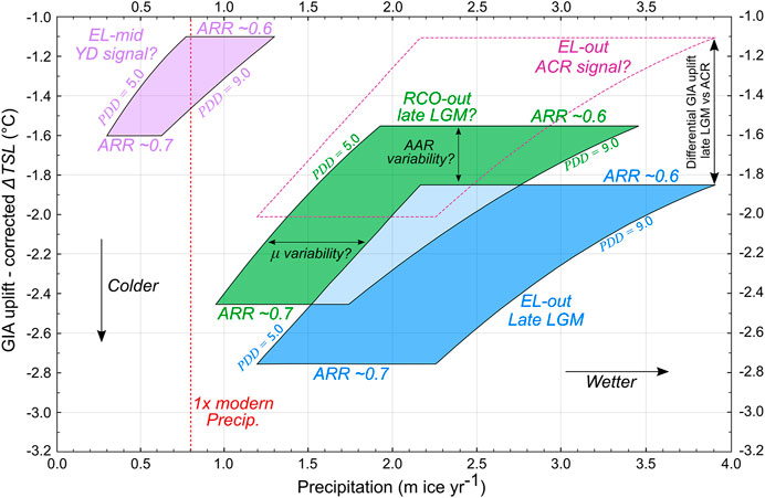
FIGURE 9. Ice-flow model temperature depression and precipitation parameter combinations for moraine-matching simulations of the EL-out (blue), EL-mid (purple) and RCO-out (green) advances/still-stands. Temperature depression values are corrected for modelled GIA-related uplift since time of advance/still-stand. Note that GIA-corrected temperature depressions include the hypothetical assumptions that the EL-mid advance/still-stand dates to the YD (∼12 ka), and the RCO-out and EL-out advances are coeval (∼18 ka). The dashed purple “SMB parameter box” denotes a hypothetical advance/still-stand of the EL glacier reaching a similar ice-front position to the EL-out advance, but dating to the ACR (∼14 ka) and thus associated with less GIA-related uplift (17.7 m).

However, our ¹⁰Be Río Corcovado moraine chronology suggest the Río Corcovado outlet glacier started to retreat from its LGM margins approximately 1.5–2 ka prior to this late-LGM return to colder/wetter conditions. Furthermore, our reconstruction of deglacial proglacial lake-level evolution and the timing of glaciolacustrine drainage shifts following the initial retreat of the Río Corcovado glacier front implies that the outlet glacier did not experience a significant re-advance towards its LGM margins during the late-LGM climatic event, at around ∼18 ka (Leger et al., 2021). The relatively short-lived (∼1.5 ka) nature of the late-LGM cooling and high precipitation event could perhaps explain the lack of a major outlet glacier re-advance, as the extensive Río Corcovado outlet glacier may require a longer duration before adjusting its geometry and advancing up a reversed slope. Alternatively, one could argue that, in this region, a negative-mass-balance-inducing feedback mechanism prevented the ice-sheet outlets from being sensitive to a late-LGM colder/wetter episode following earlier initial retreat. Based on recent investigations modelling lake-terminating mountain glaciers (e.g., Sutherland et al., 2020), we propose that the enhanced calving rates caused by large and deep proglacial lakes formed in overdeepened eastern Patagonian valleys during deglaciation were likely responsible for this glacier-climate de-coupling effect. Sensitive mountain glaciers (e.g., the EL and RCO glaciers) perched on higher massifs of the region, however, were not affected by these proglacial lakes, and were thus able to advance/stabilise in response to this late LGM cold/wet event.

5.2.2 Palaeo-Precipitation

Our numerical modelling simulations of the EL-out advance suggest a precipitation increase of between ∼50 and ∼380% greater than present at around 18.0 ± 1.15 ka (Table 5; Figures 8, 9). Furthermore, all of the RCO-out simulations also require higher-than-today precipitation (up to 338% higher than today) when constrained by PDD melt factors of between 5.0 and 9.0 mm w.e. d⁻¹°C⁻¹ and AAR values of between 0.6 and 0.7 (Table 5; Figures 8, 9). These findings evidence a positive precipitation anomaly at around 18 ka relative to today. By assuming that both glaciers were responding to the same climatic event, we can constrain the estimated precipitation range to 49–338% increases relative to the present, which represents the overlap between the EL-out and RCO-out palaeo-glacier simulations when constraining SMB identically (Figure 9). Based on comparisons with results from Patagonian LGM palaeo-precipitation proxy data and palaeo-climate models (e.g., Galloway et al., 1988; Cartwright et al., 2011; Berman et al., 2016), we consider the lower-end estimates of our resulting palaeo-precipitation range the most likely (i.e., ∼50–200% increases). Even with an equatorward-migrated SWW belt, with its core located towards 43°S, the orographic effect associated with the Patagonian Andes would still cause a rain-shadow effect, effectively starving the eastern side of the mountain front of moisture. In comparison, present-day climate displays total annual precipitation increases of more than 50% between 43°S and 49–50°S (the modern core of the SWW belt) only towards the western margin of the cordillera. Towards the centre of the Andes, this latitudinal precipitation increase is reduced to ∼20% (Garreaud et al., 2013; Fick and Hijmans., 2017). Given these known orographic effects and the location of our study site towards the eastern margin of the mountain front (71°S; Figure 1), we consider model outputs suggesting precipitation increases > ∼200%, to be less likely.

Despite the wide range of possible values that would simulate moraine-matching glacier advances, our results suggest that a local positive precipitation anomaly relative to today was required during the late-LGM. While the breakdown of the PIS and the reduction of its orographic effect may be expected to contribute to local precipitation increases, we do not consider this a primary driver because significant local ice-sheet disintegration did not occur until much later, at 16.3 ± 0.8 ka (Leger et al., 2021). Hence, we suggest that the positive precipitation anomaly identified here is consistent with the proposed hypothesis of high local SWW influence and equatorward migration of the wind belt during the late-LGM (19.5–18 ka). This latitudinal shift potentially induced positive glacier mass balances and reduced summer temperatures in northern Patagonia at the time (Denton et al., 1999; Heusser, 1983; Heusser et al., 1999; Moreno et al., 2015; 2018).

5.2.3 Palaeo-Temperatures

Our results from the EL-out simulations suggest that, after accommodating local GIA-related uplift corrections, local temperatures at around 18.0 ± 1.15 ka were between 1.9 and 2.8°C colder than today (Tables 4, 5; Figures 8, 9). The RCO-out simulations suggest a similar cooling signal of between −1.6 and −2.5°C. By validating the EL-out and RCO-out moraines to be age-equivalent, one could reduce the envelope of former temperatures to the overlap between the two simulations, resulting in a cooling of between −1.9 and −2.5°C. These figures should be treated with caution, however, as numerous assumptions and sources of uncertainty exist (Limitations and Future Work section). Firstly, we were unable to calibrate ice extents and thicknesses simulated with our modern climate estimation against modern glaciers as these do not exist in the study area. Furthermore, the lack of localised weather station data makes chosing a method for estimating atmospheric temperatures and ALR values representative of modern-day climate challenging, and this uncertainty is enhanced by the assumption that the ALR was constant over the past 18 ka, which is currently implausible to determine for certain. While we here acknowledge such uncertainties, we consider our method for estimating modern-day climate (Modern climate section) to be appropriate, and thus propose that local atmospheric temperatures were between ∼1.9 and ∼2.8°C lower than present during the late-LGM (19.5–18 ka), as suggested by our model results. This estimation overlaps the LGM mean annual temperature depression range of 2.3–4.4°C proposed for eastern Patagonia by palaeo-climate proxy data compilation and modelling using the PMIP3 model (Berman et al., 2016).

5.2.4 Younger Late-Glacial Advances/Still-Stands

There is widespread empirical evidence for glacial advances/still-stands occurring after the final disintegration of the PIS, during the Antarctic Cold Reversal (ACR) across Patagonia (Clapperton et al., 1995; Ackert et al., 2008; Glasser et al., 2011; García et al., 2012; Nimick et al., 2016; Davies et al., 2018; Sagredo et al., 2018; Reynhout et al., 2019; Mendelová et al., 2020b), New Zealand (e.g., Putnam et al., 2010), and other glacierised regions of the southern mid-latitudes such as the Kerguelen Archipelago (e.g., Jomelli et al., 2017; Charton et al., 2020). A new comprehensive ¹⁰Be moraine chronology (Soteres et al., personal communication) from the Nikita valley (43°57′48″S; 71°38′11″W), located 30 km south of the EL valley, provides robust geochronological evidence for an advance of the Nikita palaeo-glacier during the ACR (14.7–13.0 ka; Pedro et al., 2016). This re-advance reached a similar, but slightly less extensive (<500 m) glacier extent than an older advance/still-stand associated with the outermost ridges of the terminal moraine complex, which is argued to have occurred around ∼16 ka (Soteres et al., personal communication). Similarly to the EL valley, the Nikita valley also contains a smaller set of mid-valley, more subtle latero-frontal moraines located ∼1.7 km further upstream from the outermost moraines. The authors propose that these ridges were likely deposited during the Younger Dryas stadial (YD: 12.9–11.7 ka) based on TCN dating results. Such a pattern of extensive ACR moraines and more subtle but distinct YD moraines located up-valley was also observed in central Patagonia (47–48°S; Sagredo et al., 2018; Mendelová et al., 2020b). According to the geomorphological similarity and proximity of the Nikita and EL moraine records, one could speculate that the innermost terminal ridges of the EL-out moraine complex may also have been deposited during the ACR, while the smaller, mid-valley latero-frontal moraines (EL-mid) observed further up-valley could perhaps date to the YD stadial.

If those hypothetical assumptions, based solely on cross-valley morphostratigraphic comparisons, are valid, our glacier numerical modelling results could be utilised to infer that regional precipitation was likely between 50 and 380% higher than present during the ACR, and between 60% lower and 60% higher (∼40–160% of modern values) than present during the YD (Table 5; Figure 9). Such contrasting results would be in agreement with findings from regional palaeo-ecological proxy data that suggest late-glacial millennial-scale latitudinal shifts of the SWW belt induced increased and then decreased SWW influences in the southern mid-latitudes during the ACR and YD stadials, respectively (Siani et al., 2010; De Porras et al., 2012, 2014; Villa-Martínez et al., 2012; Montade et al., 2013; Moreno et al., 2018, 2019; Vilanova et al., 2019). Recent work by Skirrow et al. (2021) supports a poleward latitudinal shift of the SWW during the YD through Optically Simulated Luminescence dating of a reduction in the water supply of Río Chubut, in northeastern Patagonia. When using the modern climate estimation described in section Modern Climate. exclusively, and after including GIA-related surface uplift corrections of 17.7 and 0 m associated with EL glacier advances hypothetically timed at ∼14 ka (ACR) and ∼12 ka (YD), as suggested by the gFlex model output data (Table 4), our modelling results would suggest that local temperatures were between 1.1–2.0°C and 1.1–1.6°C lower than today during the ACR and YD stadials, respectively (Table 5; Figure 9). These inferences are close to findings reported by Sagredo et al. (2018) using ΔELA depression estimates for the extant Río Tranquilo glacier (47°S), suggesting a minimum cooling for the outermost ACR advance (13.9 ± 0.7 ka) of between 1.6 and 1.8°C. A scenario of northward SWW belt migration and local precipitation increase is also proposed by Sagredo et al. (2018) to help explain the widespread trans-Pacific and trans-latitudinal positive mass balance signal of sensitive Patagonian mountain glaciers during the ACR.

According to our model simulations, the EL-mid advance, which we speculate to date to the YD stadial, represents a ∼54% ice-volume loss and ∼37% ice-extent decrease relative to the EL-out advance dated to 18.0 ± 1.15 ka and perhaps also associated with an ACR re-advance. Given the large overlap in the estimated local palaeo-temperature ranges required during the ACR and YD scenarios, the majority of this significant ice loss would possibly have been caused by a decrease in precipitation during the YD stadial. This suggests that mountain glaciers in northeastern Patagonia were highly sensitive to variations in precipitation, most likely associated with latitudinal shifts of the SWW belt. Model simulations of the EL-mid advance require between 600 and 700 years to reach steady glacier volume (Table 5). Given the YD stadial was ∼1.2 kyr long, such inferences presume that the EL-mid moraines were potentially deposited by either a small re-advance, or a still-stand. This hypothesis is also supported by the smaller, more subtle geomorphology of the EL-mid moraines relative to the EL-out moraine complex.

It is however essential to stress that the above discussion (Younger Late-Glacial Advances/Still-Stands section) is not based on any chronological evidence, but is instead exclusively based on cross-valley comparisons and mostly aims at encouraging further work in the study region. The speculative results presented here thus await either confirmation or disproof by future glacier chronological reconstructions.

5.3 Positive Degree-Day Melt Factor Variability

Simulations of the RCO-out glacier advance suggest that, using identical SMB parameters as for simulations of the EL-out glacier advance, PDD melt factor values need to be between 1.4 and 1.7 times greater to produce moraine-matching simulations. Using identical PDD melt factors instead causes the RCO ice-front to overrun the RCO-out lateral moraines. We consider such a former glacier-front position as unlikely, as it would have caused much greater erosion of the RC III-V LGM moraine record than can be observed in the field. Assuming that both advances were most likely coeval and that climatic conditions were similar in both adjacent catchments, this offset in former ice-front extents might therefore suggest a notable difference in former surface melt rates between the two palaeo-glaciers. Geomorphological analyses reveal that, relative to the RCO valley, the EL valley is narrower, its valley slopes are steeper, and it contains a higher concentration of eroded rock slopes with large debris cones and evidence of substantial talus accretion towards their base (Figures 2, 3). We therefore suggest that former supraglacial debris cover might have been more substantial for the EL glacier than for the RCO glacier, thus potentially causing ice-surface insulation, lower surface melt-rates, and greater relative ice-extent in the ablation zone. The larger size of the EL-out relative to the RCO-out lateral moraines is potentially indicative of greater debris delivery, despite the EL glacier being smaller in surface area. Heavily debris-covered mountain glaciers are also often characterised by relatively low AARs (Benn et al., 2005). If both advances were synchronous and debris cover on the EL glacier was greater, then the AAR value associated with the RCO-out advance was likely greater than for the EL-out advance. This could explain, if excluding the hypothesis that both advances were not triggered by the same climatic event, why the two palaeo-glacier simulation sets, both constrained with AAR values of 0.6 and 0.7, do not produce identical palaeo-temperature ranges (Figure 9).

5.4 Limitations and Future Work

The outputs of our coupled SMB and ice-flow model simulations are subject to several limiting assumptions, which are as follows: 1) the SIA is appropriate for simulating the former extent of the EL and RCO glaciers. 2) The EL and RCO palaeo-glaciers were climate-sensitive and in a state of mass-balance equilibrium at the time of the reconstructed advances/still-stands. 3) All precipitation was accumulated as glacier ice, 4) the contribution of avalanching to glacier accumulation was negligible, 5) the ice was at its pressure-melting point uniformly across the glacier domain, and 6) ablation caused by sublimation or ice-front breakoff is not significant enough to be considered by our SMB parameterisation. 7) The EL and RCO glaciers were mostly free of supraglacial debris cover, and 8) the removal of valley-fill debris deposited after glacier retreat would not cause significant impacts on simulated glacier geometries and extent.

In future work, the utilisation of a high-order or Stokes model, along with a more complex SMB model, could enable revisiting and testing the impact of assumptions 1), 3), and 6), although such an approach would require significantly more computational power. Assumption 2) could be re-assessed by dating the RCO-out moraines and by generating glacier-moraine chronologies in other mountain valleys of the region. Uncertainties associated with assumption 7) and 8) could potentially be reduced in future investigations by conducting thorough sedimentological and geomorphological analyses of glaciogenic and debris deposits. Assumptions 4), and 5) however, are likely to be problematic to resolve further. SMB-derived palaeo-climate ranges could potentially be refined by improving future estimations of catchment-specific atmospheric temperatures, ALR, as well as annual and seasonal precipitation representative of modern-day climate. Finally, the dating of the innermost EL-out moraines and the EL-mid moraines is required to assess our assumption that they reflect glacial advances occurring during the ACR and YD cold intervals, respectively.

6 Conclusion

Geomorphological mapping of preserved glacial moraine complexes near the mouths of the El Loro and Río Comisario mountain valleys, northeastern Patagonia (43°S; 71°W), has evidenced former advances/still-stands of local mountain glaciers that are younger than the dated LGM advances/still-stands of the local Patagonian Ice Sheet outlet glacier, the Río Corcovado glacier.

In the El Loro valley, ¹⁰Be surface exposure dating of the inferred outermost advance of the moraine complex suggests a minimum age of 18.0 ± 1.15 ka, while another, undated moraine complex is evident further upstream, indicative of a mid-valley re-advance and/or stabilisation of the EL palaeo-glacier front.

Our findings suggest that while PIS outlet glaciers in northeastern Patagonia experienced a relatively early initial deglaciation from their LGM margins (∼19–20 ka) and no substantial late-LGM re-advances, local sensitive mountain glaciers re-advanced during the late-LGM. We propose that this glacier expansion event was triggered by the late-LGM, 1.5 kyr-long cold and wet interval (∼19.5–18 ka) recorded in other regions of Patagonia which followed the Varas Interstade (22–19.2 ka), and which preceded widespread Patagonian deglaciation (17.9–15 ka). We thus hypothesise that climatic conditions during the late-LGM were suitable for glacier expansion in northeastern Patagonia, and that the earlier onset of local PIS outlet glacier retreat at around ∼19–20 ka was likely exacerbated by non-climatic factors, such as proglacial lake formation.

We estimate site-specific cumulative surface uplift caused by Glacial Isostatic Adjustment over the past 18 ka to be approximately 130 m, while time-varying uplift rates are estimated at 9.1, 39.4 and 11.6 mm yr⁻¹ between 20–17.5, 17.5–15, and 15–12.5 ka, respectively. The impact of such uplift on ¹⁰Be production rates is less than exposure-age 1σ analytical uncertainties. Nevertheless, it requires modification of our surface mass balance-driven temperature and ELA reconstructions by −0.85°C and −131 m, respectively. Our investigation highlights that GIA-related surface elevation change is an important factor to consider in palaeo-climate investigations using glacier reconstructions. This uplift is particularly relevant in Patagonia, where low mantle viscosities drive rapid uplift following deglaciation.

Ice-flow model surface mass balance analyses suggest that regional mean annual temperatures were between 1.9 and 2.8°C lower than present at around 18.0 ± 1.15 ka, while precipitation was between ∼50 and ∼380% higher than today. Our results thus support the hypothesis of increased Southern Westerly Winds influence in northern Patagonia between ∼19.5 and ∼18 ka, resulting from an equatorward migration of the wind belt, which may have induced positive glacial mass balances across the region.

ASTER Team

Georges Aumaitre, Aix-Marseille Université, CNRS, IRD, INRAE, CEREGE, Aix-en-Provence, France; Karim Keddadouche, Aix-Marseille Université, CNRS, IRD, INRAE, CEREGE, Aix-en-Provence, France; Fawzi Zaidi, Aix-Marseille Université, CNRS, IRD, INRAE, CEREGE, Aix-en-Provence, France

Data Availability Statement

The original contributions presented in the study are included in the article/Supplementary Material, further inquiries can be directed to the corresponding author.

Ethics Statement

Written informed consent was obtained from the individual(s) for the publication of any potentially identifiable images or data included in this article.

Author Contributions

TPML: Conceptualization, Data curation, Formal analysis, Funding acquisition, Investigation, Methodology, Project administration, Software, Visualization, Writing (original draft and review and editing). ASH: Conceptualization, Methodology, Project administration, Supervision, Validation, Writing (original draft and review and editing). DG: Data curation, Investigation, Methodology, Software, Writing (original draft and review and editing). IS: Data curation, Supervision, Writing (review and editing). MV: Data curation, Methodology, Writing (review and editing). RB: Supervision, Writing (review and editing). All authors have approved the final version of the manuscript prior to submission.

Funding

This investigation is part of a University of Edinburgh E3 Doctoral Training Partnership Ph.D. studentship (award code: NE/L002558/1) awarded by the National Environment Research Council (NERC) to TPML. Our 2020 field expedition was supported by a crowd-funding campaign through the Crowd.Science fundraising platform (https://crowd.science) and a British Society for Geomorphology Postgraduate Research Grant award (BSG-2019-04) awarded to TPML in October 2019. TCN dating laboratory analyses and AMS measurements were partly funded by a Scottish Alliance for Geoscience, Environment and Society (SAGES) small grant scheme awarded to TPML in August 2020.

Conflict of Interest

The authors declare that the research was conducted in the absence of any commercial or financial relationships that could be construed as a potential conflict of interest.

The handling editor declared a past co-authorship with one of the authors ASH.

Publisher’s Note

All claims expressed in this article are solely those of the authors and do not necessarily represent those of their affiliated organizations, or those of the publisher, the editors and the reviewers. Any product that may be evaluated in this article, or claim that may be made by its manufacturer, is not guaranteed or endorsed by the publisher.

Acknowledgments

We express our most sincere gratitude towards all individuals who contributed to the https://crowd.science/crowdfunding campaign facilitating a 2020 field trip to the study site. We also thank all local landowners who authorized access and work on their properties, in particular, the Estancia Tecka (Chubut, Argentina) for enabling access to their land and private roads. Moreover, we are thankful to Pablo Tapia Gonzalez for his presence and assistance in the field. We thank Juan Luis García, María Paz Lira-Bahamonde, Mateo A. Martini and Rodrigo Soteres for their help, advice and logistical support with the overall project. We are grateful for the help of Richard S. Jones in obtaining and interpreting GIA uplift data from the iceTEA tools for exposure ages (http://ice-tea.org/en/). We thank Elaine McDougall for her preciouswork enabling efficient rock sample quartz purification and isolation. We also wish to thank Maxime Vergez for his invaluable help towards model output coding analyses and Emeritus Professor David E. Sugden for providing indispensable advice and guidance on the final manuscript. Finally, we thank the two reviewers for their thoughtful comments allowing us to improve the quality of the manuscript.

Supplementary Material

The Supplementary Material for this article can be found online at: https://www.frontiersin.org/articles/10.3389/feart.2021.751987/full#supplementary-material

Footnotes

¹http://geodesy.unr.edu/NGLStationPages/gpsnetmap/GPSNetMap_MAG.html

²Dataset: ASF DAAC 2015, ALOS PALSAR_Radiometric_Terrain_Corrected_low_res; Includes Material © JAXA/METI 2007. Accessed through https://asf.alaska.edu on 20th September 2018.

References

Ackert, R. P., Becker, R. A., Singer, B. S., Kurz, M. D., Caffee, M. W., and Mickelson, D. M. (2008). Patagonian Glacier Response during the Late Glacial-Holocene Transition. Science 321 (5887), 392–395. doi:10.1126/science.1157215

PubMed Abstract | CrossRef Full Text | Google Scholar

Adhikari, S., and Marshall, S. J. (2012). Glacier Volume-Area Relation for High-Order Mechanics and Transient Glacier States. Geophys. Res. Lett. 39 (16), a–n. doi:10.1029/2012GL052712

CrossRef Full Text | Google Scholar

Anderson, L. S., Roe, G. H., and Anderson, R. S. (2014). The Effects of Interannual Climate Variability on the Moraine Record. Geology 42 (1), 55–58. doi:10.1130/G34791.1

CrossRef Full Text | Google Scholar

Applegate, P. J., Urban, N. M., Laabs, B. J. C., Keller, K., and Alley, R. B. (2010). Modeling the Statistical Distributions of Cosmogenic Exposure Dates from Moraines. Geosci. Model. Dev. 3 (1), 293–307. doi:10.5194/gmd-3-293-2010

CrossRef Full Text | Google Scholar

Arnold, M., Merchel, S., Bourlès, D. L., Braucher, R., Benedetti, L., Finkel, R. C., et al. (2010). The French Accelerator Mass Spectrometry Facility ASTER: Improved Performance and Developments. Nucl. Instr. Methods Phys. Res. Section B: Beam Interactions Mater. Atoms 268 (11-12), 1954–1959. doi:10.1016/j.nimb.2010.02.107

CrossRef Full Text | Google Scholar

Balco, G., Stone, J. O., Lifton, N. A., and Dunai, T. J. (2008). A Complete and Easily Accessible Means of Calculating Surface Exposure Ages or Erosion Rates from 10Be and 26Al Measurements. Quat. Geochronol. 3 (3), 174–195. doi:10.1016/j.quageo.2007.12.001

CrossRef Full Text | Google Scholar

Banerjee, A., and Shankar, R. (2013). On the Response of Himalayan Glaciers to Climate Change. J. Glaciol. 59 (215), 480–490. doi:10.3189/2013JoG12J130

CrossRef Full Text | Google Scholar

Benn, D. I., Kirkbride, M. P., Owen, L. A., and Brazier, V. (2003). Glaciated valley Landsystems. Glacial Landsystems. chapter 15, 372–406.

Google Scholar

Benn, D. I., Owen, L. A., Osmaston, H. A., Seltzer, G. O., Porter, S. C., and Mark, B. (2005). Reconstruction of Equilibrium-Line Altitudes for Tropical and Sub-tropical Glaciers. Quat. Int. 138-139, 8–21. doi:10.1016/j.quaint.2005.02.003

CrossRef Full Text | Google Scholar

Berman, A. L., Silvestri, G. E., and Tonello, M. S. (2016). Differences between Last Glacial Maximum and Present-Day Temperature and Precipitation in Southern South America. Quat. Sci. Rev. 150, 221–233. doi:10.1016/j.quascirev.2016.08.025

CrossRef Full Text | Google Scholar

Bindschadler, R. (1983). The Importance of Pressurized Subglacial Water in Separation and Sliding at the Glacier Bed. J. Glaciol. 29 (101), 3–19. doi:10.3189/S0022143000005104

CrossRef Full Text | Google Scholar

Blake, W., Fischer, U. H., Bentley, C. R., and Clarke, G. K. G. (1994). Instruments and Methods: Direct Measurement of Sliding at the Glacier Bed. J. Glaciol. 40 (136), 595–599. doi:10.3189/S002214300001248X

CrossRef Full Text | Google Scholar

Bourlès, D. (1988). Etude de la géochimies de l'isotope cosmogénique ¹⁰Be et de son isotope stable ⁹Be en milieu océanique. Application à la datation des sédiments marins. Paris XI: Univ. Ph.D. thesis.

Google Scholar

Braithwaite, R. J., and Müller, F. (1980). On the Parameterization of Glacier Equilibrium Line Altitude. IAHS Publ. 126, 263–271.

Google Scholar

Braithwaite, R. J., and Zhang, Y. (2000). Sensitivity of Mass Balance of Five Swiss Glaciers to Temperature Changes Assessed by Tuning a Degree-Day Model. J. Glaciol. 46 (152), 7–14. doi:10.3189/172756500781833511

CrossRef Full Text | Google Scholar

Braucher, R., Guillou, V., Bourlès, D. L., Arnold, M., Aumaître, G., Keddadouche, K., et al. (2015). Preparation of ASTER In-House 10Be/9Be Standard Solutions. Nucl. Instr. Methods Phys. Res. Section B: Beam Interactions Mater. Atoms 361, 335–340. doi:10.1016/j.nimb.2015.06.012

CrossRef Full Text | Google Scholar

Budd, W. F., Keage, P. L., and Blundy, N. A. (1979). Empirical Studies of Ice Sliding. J. Glaciol. 23 (89), 157–170. doi:10.3189/S0022143000029804

CrossRef Full Text | Google Scholar

Caldenius, C. C. Z. (1932). Las glaciaciones cuaternarias en la patagonia y tierra del fuego. Geografiska Annaler 14, 1–164. doi:10.1080/20014422.1932.11880545

CrossRef Full Text | Google Scholar

Caniupán, M., Lamy, F., Lange, C. B., Kaiser, J., Arz, H., Kilian, R., et al. (2011). Millennial-scale Sea Surface Temperature and Patagonian Ice Sheet Changes off Southernmost Chile (53°S) over the Past ∼60 Kyr. Paleoceanography 26 (3), a–n. doi:10.1029/2010PA002049

CrossRef Full Text | Google Scholar

Cartwright, A., Quade, J., Stine, S., Adams, K. D., Broecker, W., and Cheng, H. (2011). Chronostratigraphy and lake-level Changes of Laguna Cari-Laufquén, Río Negro, Argentina. Quat. Res. 76 (3), 430–440. doi:10.1016/j.yqres.2011.07.002

CrossRef Full Text | Google Scholar

Charton, J., Jomelli, V., Schimmelpfennig, I., Verfaillie, D., Favier, V., Mokadem, F., et al. (2021). A Debris-Covered Glacier at Kerguelen (49° S, 69° E) Over the Past 15 000 years. Antarctic Sci. 33 (1), 103–115. doi:10.1017/S0954102020000541

CrossRef Full Text | Google Scholar

Chmeleff, J., von Blanckenburg, F., Kossert, K., and Jakob, D. (2010). Determination of the 10Be Half-Life by Multicollector ICP-MS and Liquid Scintillation Counting. Nucl. Instr. Methods Phys. Res. Section B: Beam Interactions Mater. Atoms 268 (2), 192–199. doi:10.1016/j.nimb.2009.09.012

CrossRef Full Text | Google Scholar

Clapperton, C. M. (1993). Quaternary Geology and Geomorphology of South America, 25. Amsterdam etc: Elsevier.

Google Scholar

Clapperton, C. M. (1990). Quaternary Glaciations in the Southern Hemisphere: an Overview. Quat. Sci. Rev. 9 (2-3), 299–304. doi:10.1016/0277-3791(90)90024-5

CrossRef Full Text | Google Scholar

Clapperton, C. M., Sugden, D. E., Kaufman, D. S., and McCulloch, R. D. (1995). The Last Glaciation in central Magellan Strait, Southernmost Chile. Quat. Res. 44 (2), 133–148. doi:10.1006/qres.1995.1058

CrossRef Full Text | Google Scholar

Cohen, D., Hooke, R. L., Iverson, N. R., and Kohler, J. (2000). Sliding of Ice Past an Obstacle at Engabreen, Norway. J. Glaciol. 46 (155), 599–610. doi:10.3189/172756500781832747

CrossRef Full Text | Google Scholar

Cohen, D., Iverson, N. R., Hooyer, T. S., Fischer, U. H., Jackson, M., and Moore, P. L. (2005). Debris-bed Friction of Hard-Bedded Glaciers. J. Geophys. Res. 110 (F2). doi:10.1029/2004JF000228

CrossRef Full Text | Google Scholar

Cuffey, K., and Paterson, W. S. B. (2010). The Physics of Glaciers. Burlington, MA, USA: Elsevier, Butterworth-Heineman, 704.

Google Scholar

Darvill, C. M., Bentley, M. J., Stokes, C. R., and Shulmeister, J. (2016). The Timing and Cause of Glacial Advances in the Southern Mid-latitudes during the Last Glacial Cycle Based on a Synthesis of Exposure Ages from Patagonia and New Zealand. Quat. Sci. Rev. 149, 200–214. doi:10.1016/j.quascirev.2016.07.024

CrossRef Full Text | Google Scholar

Davies, B. J., Darvill, C. M., Lovell, H., Bendle, J. M., Dowdeswell, J. A., Fabel, D., et al. (2020). The Evolution of the Patagonian Ice Sheet from 35 Ka to the Present Day (PATICE). Earth-Science Rev. 204, 103152. doi:10.1016/j.earscirev.2020.103152

CrossRef Full Text | Google Scholar

Davies, B. J., Thorndycraft, V. R., Fabel, D., and Martin, J. R. V. (2018). Asynchronous Glacier Dynamics during the Antarctic Cold Reversal in central Patagonia. Quat. Sci. Rev. 200, 287–312. doi:10.1016/J.QUASCIREV.2018.09.025

CrossRef Full Text | Google Scholar

De Angelis, H. (2014). Hypsometry and Sensitivity of the Mass Balance to Changes in Equilibrium-Line Altitude: the Case of the Southern Patagonia Icefield. J. Glaciol. 60 (219), 14–28. doi:10.3189/2014JoG13J127

CrossRef Full Text | Google Scholar

De Porras, M. E., Maldonado, A., Abarzúa, A. M., Cárdenas, M. L., Francois, J. P., Martel-Cea, A., et al. (2012). Postglacial Vegetation, Fire and Climate Dynamics at Central Chilean Patagonia (Lake Shaman, 44°S). Quat. Sci. Rev. 50, 71–85. doi:10.1016/j.quascirev.2012.06.015

CrossRef Full Text | Google Scholar

De Porras, M. E., Maldonado, A., Quintana, F. A., Martel-Cea, A., Reyes, O., and Méndez, C. (2014). Environmental and Climatic Changes in central Chilean Patagonia since the Late Glacial (Mallín El Embudo, 44° S). Clim. Past 10 (3), 1063–1078. doi:10.5194/cp-10-1063-2014

CrossRef Full Text | Google Scholar

Denton, G. H., Lowell, T. V., Heusser, C. J., Schlüchter, C., Andersen, B. G., Heusser, L. E., et al. (1999). Geomorphology, Stratigraphy, and Radiocarbon Chronology of LlanquihueDrift in the Area of the Southern Lake District, Seno Reloncavi, and Isla Grande de Chiloe, Chile. Geografiska Annaler A 81 (2), 167–229. doi:10.1111/j.0435-3676.1999.00057.x

CrossRef Full Text | Google Scholar

Denton, G. H., Putnam, A. E., Russell, J. L., Barrell, D. J. A., Schaefer, J. M., Kaplan, M. R., et al. (2021). The Zealandia Switch: Ice Age Climate Shifts Viewed from Southern Hemisphere Moraines. Quat. Sci. Rev. 257, 106771. doi:10.1016/j.quascirev.2020.106771

CrossRef Full Text | Google Scholar

Doughty, A. M., Schaefer, J. M., Putnam, A. E., Denton, G. H., Kaplan, M. R., Barrell, D. J. A., et al. (2015). Mismatch of Glacier Extent and Summer Insolation in Southern Hemisphere Mid-latitudes. Geology 43 (5), 407–410. doi:10.1130/G36477.1

CrossRef Full Text | Google Scholar

Douglass, D. C., Singer, B., Ackert, R. P., Kaplan, M. R., and Caffee, M. W. (2007). “Constraining Boulder Erosion Rates and Ages of Mid-pleistocene Moraines in Lago Buenos Aires, Argentina,” in GSA Abstracts and Programs Northeastern Section 42nd Annual Meeting, Lago Buenos Aires, Argentina.

Google Scholar

Engelhardt, H. F., Harrison, W. D., and Kamb, B. (1978). Basal Sliding and Conditions at the Glacier Bed as Revealed by Bore-Hole Photography. J. Glaciol. 20 (84), 469–508. doi:10.3189/S002214300002089X

CrossRef Full Text | Google Scholar

Fick, S. E., and Hijmans, R. J. (2017). WorldClim 2: New 1‐km Spatial Resolution Climate Surfaces for Global Land Areas. Int. J. Climatol 37 (12), 4302–4315. doi:10.1002/joc.5086

CrossRef Full Text | Google Scholar

Galloway, R. W., Markgraf, V., and Bradbury, J. P. (1988). Dating Shorelines of Lakes in Patagonia, Argentina. J. South Am. Earth Sci. 1 (2), 195–198. doi:10.1016/0895-9811(88)90037-5

CrossRef Full Text | Google Scholar

García, J.-L., Maldonado, A., de Porras, M. E., Nuevo Delaunay, A., Reyes, O., Ebensperger, C. A., et al. (2019). Early Deglaciation and Paleolake History of Río Cisnes Glacier, Patagonian Ice Sheet (44°S). Quat. Res. 91 (1), 194–217. doi:10.1016/10.1017/qua.2018.93

CrossRef Full Text | Google Scholar

García, J. L., Kaplan, M. R., Hall, B. L., Schaefer, J. M., Vega, R. M., Schwartz, R., et al. (2012). Glacier Expansion in Southern Patagonia throughout the Antarctic Cold Reversal. Geology 40 (9), 859–862. doi:10.1130/G33164.1

CrossRef Full Text | Google Scholar

Garreaud, R., Lopez, P., Minvielle, M., and Rojas, M. (2013). Large-scale Control on the Patagonian Climate. J. Clim. 26 (1), 215–230. doi:10.1175/JCLI-D-12-00001.1

CrossRef Full Text | Google Scholar

Glasser, N. F., Jansson, K. N., Goodfellow, B. W., De Angelis, H., Rodnight, H., and Rood, D. H. (2011). Cosmogenic Nuclide Exposure Ages for Moraines in the Lago San Martin Valley, Argentina. Quat. Res. 75 (3), 636–646. doi:10.1016/j.yqres.2010.11.005

CrossRef Full Text | Google Scholar

Glasser, N. F., Jansson, K. N., Harrison, S., and Kleman, J. (2008). The Glacial Geomorphology and Pleistocene History of South America between 38°S and 56°S. Quat. Sci. Rev. 27 (3-4), 365–390. doi:10.1016/10.1016/j.quascirev.2007.11.011

CrossRef Full Text | Google Scholar

Gosse, J. C., and Phillips, F. M. (2001). Terrestrial In Situ Cosmogenic Nuclides: Theory and Application. Quat. Sci. Rev. 20 (14), 1475–1560. doi:10.1016/S0277-3791(00)00171-2

CrossRef Full Text | Google Scholar

Gowan, E. J., Zhang, X., Khosravi, S., Rovere, A., Stocchi, P., Hughes, A. L. C., et al. (2021). A New Global Ice Sheet Reconstruction for the Past 80 000 Years. Nat. Commun. 12 (1), 1–9. doi:10.1038/s41467-021-21469-w

PubMed Abstract | CrossRef Full Text | Google Scholar

Hall, B. L., Porter, C. T., Denton, G. H., Lowell, T. V., and Bromley, G. R. M. (2013). Extensive Recession of Cordillera Darwin Glaciers in Southernmost South America during Heinrich Stadial 1. Quat. Sci. Rev. 62, 49–55. doi:10.1016/j.quascirev.2012.11.026

CrossRef Full Text | Google Scholar

Haller, M., Lech, R. R., Martinez, O. A., Meister, C. M., and Page, S. M. (2003). Hoja Geologica 4373IV/III, Trevelin, Provincia del Chubut. Programa Nacional de Cartas Geologicas de la Republica Argentina, 1:250.000. Buenos Aires: Servicio Geologico Nacional.

Google Scholar

Hein, A. S., Cogez, A., Darvill, C. M., Mendelová, M., Kaplan, M. R., Herman, F., et al. (2017). Regional Mid-pleistocene Glaciation in central Patagonia. Quat. Sci. Rev. 164, 77–94. doi:10.1016/j.quascirev.2017.03.023

CrossRef Full Text | Google Scholar

Hein, A. S., Hulton, N. R. J., Dunai, T. J., Sugden, D. E., Kaplan, M. R., and Xu, S. (2010). The Chronology of the Last Glacial Maximum and Deglacial Events in central Argentine Patagonia. Quat. Sci. Rev. 29 (9-10), 1212–1227. doi:10.1016/j.quascirev.2010.01.020

CrossRef Full Text | Google Scholar

Heusser, C. J., Heusser, L. E., and Lowell, T. V. (1999). Paleoecology of The Southern Chilean Lake District-Isla Grande de Chiloe During Middle-late Llanquihue Glaciation and Deglaciation. Geografiska Annaler A 81, 231–284. doi:10.1111/j.0435-3676.1999.00058.x

CrossRef Full Text | Google Scholar

Heusser, C. J. (1983). Quaternary pollen record from laguna de Tagua Tagua, Chile. Science 219 (4591), 1429–1432. doi:10.1126/science.219.4591.1429

PubMed Abstract | CrossRef Full Text | Google Scholar

Heyman, J., Stroeven, A. P., Harbor, J. M., and Caffee, M. W. (2011). Too Young or Too Old: Evaluating Cosmogenic Exposure Dating Based on an Analysis of Compiled boulder Exposure Ages. Earth Planet. Sci. Lett. 302 (1-2), 71–80. doi:10.1016/j.epsl.2010.11.040

CrossRef Full Text | Google Scholar

Hock, R. (2003). Temperature index Melt Modelling in Mountain Areas. J. Hydrol. 282 (1-4), 104–115. doi:10.1016/S0022-1694(03)00257-9

CrossRef Full Text | Google Scholar

Hubbard, A., Hein, A. S., Kaplan, M. R., Hulton, N. R. j., and Glasser, N. (2005). A Modelling Reconstruction of the Last Glacial Maximum Ice Sheet and its Deglaciation in the Vicinity of the Northern Patagonian Icefield, South America. Geografiska Annaler: Ser. A, Phys. Geogr. 87 (2), 375–391. doi:10.1111/j.0435-3676.2005.00264.x

CrossRef Full Text | Google Scholar

Huss, M., Sugiyama, S., Bauder, A., and Funk, M. (2007). Retreat Scenarios of Unteraargletscher, Switzerland, Using a Combined Ice-Flow Mass-Balance Model. Arctic, Antarctic, Alpine Res. 39 (3), 422–431. doi:10.1657/1523-0430(06-036)[HUSS]2.0.CO;2

CrossRef Full Text | Google Scholar

Hutter, K. (1983). Theoretical Glaciology: Material Science of Ice and the Mechanics of Glaciers and Ice Sheets. Dordrecht, Netherlands: Kluwer Academic Publishers.

Google Scholar

Ivins, E. R., and James, T. S. (2004). Bedrock Response to Llanquihue Holocene and Present-Day Glaciation in Southernmost South America. Geophys. Res. Lett. 31 (24). doi:10.1029/2004GL021500

CrossRef Full Text | Google Scholar

Jomelli, V., Mokadem, F., Schimmelpfennig, I., Chapron, E., Rinterknecht, V., Favier, V., et al. (2017). Sub-Antarctic Glacier Extensions in the Kerguelen Region (49°S, Indian Ocean) over the Past 24,000 Years Constrained by 36 Cl Moraine Dating. Quat. Sci. Rev. 162, 128–144. doi:10.1016/j.quascirev.2017.03.010

CrossRef Full Text | Google Scholar

Jones, R. S., Small, D., Cahill, N., Bentley, M. J., and Whitehouse, P. L. (2019a). iceTEA: Tools for Plotting and Analysing Cosmogenic-Nuclide Surface-Exposure Data from Former Ice Margins. Quat. Geochronol. 51, 72–86. doi:10.1016/j.quageo.2019.01.001

CrossRef Full Text | Google Scholar

Jones, R. S., Whitehouse, P. L., Bentley, M. J., Small, D., and Dalton, A. S. (2019b). Impact of Glacial Isostatic Adjustment on Cosmogenic Surface-Exposure Dating. Quat. Sci. Rev. 212, 206–212. doi:10.1016/j.quascirev.2019.03.012

CrossRef Full Text | Google Scholar

Jouvet, G., and Funk, M. (2014). Modelling the Trajectory of the Corpses of Mountaineers Who Disappeared in 1926 on Aletschgletscher, Switzerland. J. Glaciol. 60 (220), 255–261. doi:10.3189/2014JoG13J156

CrossRef Full Text | Google Scholar

Kaiser, J., Lamy, F., Arz, H. W., and Hebbeln, D. (2007). Dynamics of the Millennial-Scale Sea Surface Temperature and Patagonian Ice Sheet Fluctuations in Southern Chile during the Last 70kyr (ODP Site 1233). Quat. Int. 161 (1), 77–89. doi:10.1016/j.quaint.2006.10.024

CrossRef Full Text | Google Scholar

Kaplan, M. R., Coronato, A., Hulton, N. R. J., Rabassa, J. O., Kubik, P. W., and Freeman, S. P. H. T. (2007). Cosmogenic Nuclide Measurements in Southernmost South America and Implications for Landscape Change. Geomorphology 87 (4), 284–301. doi:10.1016/j.geomorph.2006.10.005

CrossRef Full Text | Google Scholar

Kaplan, M. R., Fogwill, C. J., Sugden, D. E., Hulton, N. R. J., Kubik, P. W., and Freeman, S. P. H. T. (2008). Southern Patagonian Glacial Chronology for the Last Glacial Period and Implications for Southern Ocean Climate. Quat. Sci. Rev. 27 (3-4), 284–294. doi:10.1016/j.quascirev.2007.09.013

CrossRef Full Text | Google Scholar

Kern, Z., and László, P. (2010). Size Specific Steady-State Accumulation-Area Ratio: an Improvement for Equilibrium-Line Estimation of Small Palaeoglaciers. Quat. Sci. Rev. 29 (19-20), 2781–2787. doi:10.1016/j.quascirev.2010.06.033

CrossRef Full Text | Google Scholar

Korschinek, G., Bergmaier, A., Faestermann, T., Gerstmann, U. C., Knie, K., Rugel, G., et al. (2010). A New Value for the Half-Life of 10Be by Heavy-Ion Elastic Recoil Detection and Liquid Scintillation Counting. Nucl. Instr. Methods Phys. Res. Section B: Beam Interactions Mater. Atoms 268 (2), 187–191. doi:10.1016/j.nimb.2009.09.020

CrossRef Full Text | Google Scholar

Lal, D. (1991). Cosmic ray Labeling of Erosion Surfaces: In Situ Nuclide Production Rates and Erosion Models. Earth Planet. Sci. Lett. 104, 424–439. doi:10.1016/0012-821X(91)90220-C

CrossRef Full Text | Google Scholar

Lamy, F., Kaiser, J., Arz, H. W., Hebbeln, D., Ninnemann, U., Timm, O., et al. (2007). Modulation of the Bipolar Seesaw in the Southeast Pacific during Termination 1. Earth Planet. Sci. Lett. 259, 400–413. doi:10.1016/j.epsl.2007.04.040

CrossRef Full Text | Google Scholar

Lamy, F., Kaiser, J., Ninnemann, U., Hebbeln, D., Arz, H. W., and Stoner, J. (2004). Antarctic Timing of Surface Water Changes off Chile and Patagonian Ice Sheet Response. Science 304 (5679), 1959–1962. doi:10.1126/science.1097863

PubMed Abstract | CrossRef Full Text | Google Scholar

Lange, H., Casassa, G., Ivins, E. R., Schröder, L., Fritsche, M., Richter, A., et al. (2014). Observed Crustal Uplift Near the Southern Patagonian Icefield Constrains Improved Viscoelastic Earth Models. Geophys. Res. Lett. 41 (3), 805–812. doi:10.1002/2013GL058419

CrossRef Full Text | Google Scholar

Leger, T. P. M., Hein, A. S., Bingham, R. G., Martini, M. A., Soteres, R. L., Sagredo, E. A., et al. (2020). The Glacial Geomorphology of the Río Corcovado, Río Huemul and Lago Palena/General Vintter Valleys, Northeastern Patagonia (43°S, 71°W). J. Maps 16 (2), 651–668. doi:10.1080/17445647.2020.1794990

CrossRef Full Text | Google Scholar

Leger, T. P., Hein, A. S., Bingham, R. G., Rodés, Á., Fabel, D., and Smedley, R. K. (2021). Geomorphology and ¹⁰Be Chronology of the Last Glacial Maximum and Deglaciation in NORTHEASTERN PATAGONIA, 43°S–71°W. Quat. Sci. Rev. 272, 107194. doi:10.1016/j.quascirev.2021.107194

CrossRef Full Text | Google Scholar

Lifton, N., Sato, T., and Dunai, T. J. (2014). Scaling In Situ Cosmogenic Nuclide Production Rates Using Analytical Approximations to Atmospheric Cosmic-ray Fluxes. Earth Planet. Sci. Lett. 386, 149–160. doi:10.1016/j.epsl.2013.10.052

CrossRef Full Text | Google Scholar

Lopes dos Santos, R. A., Spooner, M. I., Barrows, T. T., De Deckker, P., Sinninghe Damsté, J. S., and Schouten, S. (2013). Comparison of Organic (UK'37, TEXH86, LDI) and Faunal Proxies (Foraminiferal Assemblages) for Reconstruction of Late Quaternary Sea Surface Temperature Variability from Offshore southeastern Australia. Paleoceanography 28 (3), 377–387. doi:10.1002/palo.20035

CrossRef Full Text | Google Scholar

Martínez, O., Coronato, A., and Rabassa, J. (2011). “Pleistocene Glaciations in Northern Patagonia, Argentina: an Updated Review,” in Developments in Quaternary Sciences (Elsevier), 15, 729–734. doi:10.1016/b978-0-444-53447-7.00052-0

CrossRef Full Text | Google Scholar

Mashiotta, T. A., Lea, D. W., and Spero, H. J. (1999). Glacial-interglacial Changes in Subantarctic Sea Surface Temperature and δ18O-water Using Foraminiferal Mg. Earth Planet. Sci. Lett. 170 (4), 417–432. doi:10.1016/S0012-821X(99)00116-8

CrossRef Full Text | Google Scholar

Mendelová, M., Hein, A. S., Rodés, Á., Smedley, R. K., and Xu, S. (2020b). Glacier Expansion in central Patagonia during the Antarctic Cold Reversal Followed by Retreat and Stabilisation during the Younger Dryas. Quat. Sci. Rev. 227, 106047. doi:10.1016/j.quascirev.2019.106047

CrossRef Full Text | Google Scholar

Mendelová, M., Hein, A. S., Rodés, Á., and Xu, S. (2020a). Extensive Mountain Glaciation in central Patagonia during Marine Isotope Stage 5. Quat. Sci. Rev. 227, 105996. doi:10.1016/j.quascirev.2019.105996

CrossRef Full Text | Google Scholar

Mercer, J. H. (1972). Chilean Glacial Chronology 20,000 to 11,000 Carbon-14 Years Ago: Some Global Comparisons. Science 176 (4039), 1118–1120. doi:10.1210/jcem-10-10-136110.1126/science.176.4039.1118

PubMed Abstract | CrossRef Full Text | Google Scholar

Mercer, J. H. (1976). Glacial History of Southernmost South America. Quat. Res. 6 (2), 125–166. doi:10.1016/0033-5894(76)90047-8

CrossRef Full Text | Google Scholar

Mercer, J. H. (1984). Simultaneous Climatic Change in Both Hemispheres and Similar Bipolar Interglacial Warming: Evidence and Implications. Clim. Process. Clim. sensitivity 29, 307–313. doi:10.1029/GM029p0307

CrossRef Full Text | Google Scholar

Millan, R., Mouginot, J., Rabatel, A., Jeong, S., Cusicanqui, D., Derkacheva, A., et al. (2019). Mapping Surface Flow Velocity of Glaciers at Regional Scale Using a Multiple Sensors Approach. Remote Sensing 11 (21), 2498. doi:10.3390/rs11212498

CrossRef Full Text | Google Scholar

Montade, V., Combourieu Nebout, N., Kissel, C., Haberle, S. G., Siani, G., and Michel, E. (2013). Vegetation and Climate Changes during the Last 22,000yr from a marine Core Near Taitao Peninsula, Southern Chile. Palaeogeogr. Palaeoclimatol. Palaeoecol. 369, 335–348. doi:10.1016/j.palaeo.2012.11.001

CrossRef Full Text | Google Scholar

Moreno, P. I., Denton, G. H., Moreno, H., Lowell, T. V., Putnam, A. E., and Kaplan, M. R. (2015). Radiocarbon Chronology of the Last Glacial Maximum and its Termination in Northwestern Patagonia. Quat. Sci. Rev. 122, 233–249. doi:10.1016/j.quascirev.2015.05.027

CrossRef Full Text | Google Scholar

Moreno, P. I., Simi, E., Villa-Martínez, R. P., and Vilanova, I. (2019). Early Arboreal Colonization, Postglacial Resilience of Deciduous Nothofagus Forests, and the Southern Westerly Wind Influence in central-east Andean Patagonia. Quat. Sci. Rev. 218, 61–74. doi:10.1016/j.quascirev.2019.06.004

CrossRef Full Text | Google Scholar

Moreno, P. I., Videla, J., Valero-Garcés, B., Alloway, B. V., and Heusser, L. E. (2018). A Continuous Record of Vegetation, Fire-Regime and Climatic Changes in Northwestern Patagonia Spanning the Last 25,000 Years. Quat. Sci. Rev. 198, 15–36. doi:10.1016/j.quascirev.2018.08.013

CrossRef Full Text | Google Scholar

Murray, D. S., Carlson, A. E., Singer, B. S., Anslow, F. S., He, F., Caffee, M., et al. (2012). Northern Hemisphere Forcing of the Last Deglaciation in Southern Patagonia. Geology 40 (7), 631–634. doi:10.1130/G32836.1

CrossRef Full Text | Google Scholar

Nimick, D. A., McGrath, D., Mahan, S. A., Friesen, B. A., and Leidich, J. (2016). Latest Pleistocene and Holocene Glacial Events in the Colonia valley, Northern Patagonia Icefield, Southern Chile. J. Quat. Sci. 31 (6), 551–564. doi:10.1002/jqs.2847

CrossRef Full Text | Google Scholar

Osmaston, H. (2005). Estimates of Glacier Equilibrium Line Altitudes by the Area×Altitude, the Area×Altitude Balance Ratio and the Area×Altitude Balance Index Methods and Their Validation. Quat. Int. 138-139, 22–31. doi:10.1016/j.quaint.2005.02.004

CrossRef Full Text | Google Scholar

Pedro, J. B., Bostock, H. C., Bitz, C. M., He, F., Vandergoes, M. J., Steig, E. J., et al. (2016). The Spatial Extent and Dynamics of the Antarctic Cold Reversal. Nat. Geosci 9 (1), 51–55. doi:10.1038/ngeo2580

CrossRef Full Text | Google Scholar

Pellitero, R., Rea, B. R., Spagnolo, M., Bakke, J., Hughes, P., Ivy-Ochs, S., et al. (2015). A GIS Tool for Automatic Calculation of Glacier Equilibrium-Line Altitudes. Comput. Geosciences 82, 55–62. doi:10.1016/j.cageo.2015.05.005

CrossRef Full Text | Google Scholar

Pellitero, R., Rea, B. R., Spagnolo, M., Bakke, J., Ivy-Ochs, S., Frew, C. R., et al. (2016). GlaRe, a GIS Tool to Reconstruct the 3D Surface of Palaeoglaciers. Comput. Geosciences 94, 77–85. doi:10.1016/j.cageo.2016.06.008

CrossRef Full Text | Google Scholar

Peltier, C., Kaplan, M. R., Birkel, S. D., Soteres, R. L., Sagredo, E. A., Aravena, J. C., et al. (2021). The Large MIS 4 and Long MIS 2 Glacier Maxima on the Southern Tip of South America. Quat. Sci. Rev. 262, 106858. doi:10.1016/j.quascirev.2021.106858

CrossRef Full Text | Google Scholar

Peltier, W. R., Argus, D. F., and Drummond, R. (2015). Space Geodesy Constrains Ice Age Terminal Deglaciation: The Global ICE-6G_C (VM5a) Model. J. Geophys. Res. Solid Earth 120 (1), 450–487. doi:10.1002/2014JB011176

CrossRef Full Text | Google Scholar

Putkonen, J., and Swanson, T. (2003). Accuracy of Cosmogenic Ages for Moraines. Quat. Res. 59 (2), 255–261. doi:10.1016/S0033-5894(03)00006-1

CrossRef Full Text | Google Scholar

Putnam, A. E., Denton, G. H., Schaefer, J. M., Barrell, D. J. A., Andersen, B. G., Finkel, R. C., et al. (2010). Glacier advance in Southern Middle-Latitudes during the Antarctic Cold Reversal. Nat. Geosci 3 (10), 700–704. doi:10.1038/ngeo962

CrossRef Full Text | Google Scholar

Putnam, A. E., Schaefer, J. M., Denton, G. H., Barrell, D. J. A., Andersen, B. G., Koffman, T. N. B., et al. (2013). Warming and Glacier Recession in the Rakaia valley, Southern Alps of New Zealand, during Heinrich Stadial 1. Earth Planet. Sci. Lett. 382, 98–110. doi:10.1016/j.epsl.2013.09.005

CrossRef Full Text | Google Scholar

Reynhout, S. A., Sagredo, E. A., Kaplan, M. R., Aravena, J. C., Martini, M. A., Moreno, P. I., et al. (2019). Holocene Glacier Fluctuations in Patagonia Are Modulated by Summer Insolation Intensity and Paced by Southern Annular Mode-like Variability. Quat. Sci. Rev. 220, 178–187. doi:10.1016/j.quascirev.2019.05.029

CrossRef Full Text | Google Scholar

Richter, A., Ivins, E., Lange, H., Mendoza, L., Schröder, L., Hormaechea, J. L., et al. (2016). Crustal Deformation across the Southern Patagonian Icefield Observed by GNSS. Earth Planet. Sci. Lett. 452, 206–215. doi:10.1016/j.epsl.2016.07.042

CrossRef Full Text | Google Scholar

Rivera, A., Bown, F., Carrión, D., and Zenteno, P. (2012). Glacier Responses to Recent Volcanic Activity in Southern Chile. Environ. Res. Lett. 7 (1), 014036. doi:10.1088/1748-9326/7/1/014036

CrossRef Full Text | Google Scholar

Roe, G. H., and O’Neal, M. A. (2009). The Response of Glaciers to Intrinsic Climate Variability: Observations and Models of Late-Holocene Variations in the Pacific Northwest. J. Glaciol. 55 (193), 839–854. doi:10.3189/002214309790152438

CrossRef Full Text | Google Scholar

Roe, G. H. (2011). What Do Glaciers Tell Us about Climate Variability and Climate Change. J. Glaciol. 57 (203), 567–578. doi:10.3189/002214311796905640

CrossRef Full Text | Google Scholar

Sagredo, E. A., Kaplan, M. R., Araya, P. S., Lowell, T. V., Aravena, J. C., Moreno, P. I., et al. (2018). Trans-pacific Glacial Response to the Antarctic Cold Reversal in the Southern Mid-latitudes. Quat. Sci. Rev. 188, 160–166. doi:10.1016/j.quascirev.2018.01.011

CrossRef Full Text | Google Scholar

Shulmeister, J., Fink, D., Hyatt, O. M., Thackray, G. D., and Rother, H. (2010). Cosmogenic 10Be and 26Al Exposure Ages of Moraines in the Rakaia Valley, New Zealand and the Nature of the Last Termination in New Zealand Glacial Systems. Earth Planet. Sci. Lett. 297 (3-4), 558–566. doi:10.1016/j.epsl.2010.07.007

CrossRef Full Text | Google Scholar

Shulmeister, J., Thackray, G. D., Rittenour, T. M., Fink, D., and Patton, N. R. (2019). The Timing and Nature of the Last Glacial Cycle in New Zealand. Quat. Sci. Rev. 206, 1–20. doi:10.1016/j.quascirev.2018.12.020

CrossRef Full Text | Google Scholar

Siani, G., Colin, C., Michel, E., Carel, M., Richter, T., Kissel, C., et al. (2010). Late Glacial to Holocene Terrigenous Sediment Record in the Northern Patagonian Margin: Paleoclimate Implications. Palaeogeogr. Palaeoclimatol. Palaeoecol. 297 (1), 26–36. doi:10.1016/j.palaeo.2010.07.011

CrossRef Full Text | Google Scholar

Skirrow, G. K., Smedley, R. K., Chiverrell, R. C., and Hooke, J. M. (2021). Planform Change of the Río Chubut (∼42°S, ∼70°W, Argentina) in Response to Climate Drivers in the Southern Andes. Geomorphology 393, 107924. doi:10.1016/j.geomorph.2021.107924

CrossRef Full Text | Google Scholar

Stone, J. O. (2000). Air Pressure and Cosmogenic Isotope Production. J. Geophys. Res. 105 (B10), 23753–23759. doi:10.1029/2000jb900181

CrossRef Full Text | Google Scholar

Sun, Y., Xu, X., Zhang, L., Liu, J., Zhang, X., Li, J., et al. (2020). Numerical Reconstruction of Three Holocene Glacial Events in Qiangyong Valley, Southern Tibetan Plateau and Their Implication for Holocene Climate Changes. Water 12 (11), 3205. doi:10.3390/w12113205

CrossRef Full Text | Google Scholar

Sutherland, J. L., Carrivick, J. L., Gandy, N., Shulmeister, J., Quincey, D. J., and Cornford, S. L. (2020). Proglacial Lakes Control Glacier Geometry and Behavior during Recession. Geophys. Res. Lett. 47, e2020GL088865. doi:10.1029/2020gl088865

CrossRef Full Text | Google Scholar

Vilanova, I., Moreno, P. I., Miranda, C. G., and Villa-Martínez, R. P. (2019). The Last Glacial Termination in the Coyhaique Sector of central Patagonia. Quat. Sci. Rev. 224, 105976. doi:10.1016/j.quascirev.2019.105976

CrossRef Full Text | Google Scholar

Villa-Martínez, R., Moreno, P. I., and Valenzuela, M. A. (2012). Deglacial and Postglacial Vegetation Changes on the Eastern Slopes of the central Patagonian Andes (47°S). Quat. Sci. Rev. 32, 86–99. doi:10.1016/j.quascirev.2011.11.008

CrossRef Full Text | Google Scholar

Vivian, R. (1967). Le Glacier Blanc. rga 55 (4), 729–732. doi:10.3406/rga.1967.3351

CrossRef Full Text | Google Scholar

Vivian, R., and Volle, L. (1967). Le Glacier d'Arsine. rga 55 (2), 396–400. doi:10.3406/rga.1967.3325

CrossRef Full Text | Google Scholar

Wallace, J. M., and Hobbs, P. V. (2006). Atmospheric Science: An Introductory Survey, 92. Elsevier.

Google Scholar

Weertman, J. (1957). On the Sliding of Glaciers. J. Glaciol. 3 (21), 33–38. doi:10.3189/s0022143000024709

CrossRef Full Text | Google Scholar

Wendt, I., and Carl, C. (1991). The Statistical Distribution of the Mean Squared Weighted Deviation. Chem. Geology. Isotope Geosci. Section 86 (4), 275–285. doi:10.1016/0168-9622(91)90010-T

CrossRef Full Text | Google Scholar

Wickert, A. D. (2015). Open-source Modular Solutions for Flexural Isostasy: gFlex v1.0. Geosci. Model. Dev. 9 (6), 997–1017. doi:10.5194/gmd-9-997-2016

CrossRef Full Text | Google Scholar

Wijngaard, R. R., Steiner, J. F., Kraaijenbrink, P. D. A., Klug, C., Adhikari, S., Banerjee, A., et al. (2019). Modeling the Response of the Langtang Glacier and the Hintereisferner to a Changing Climate since the Little Ice Age. Front. Earth Sci. 7, 143. doi:10.3389/feart.2019.00143

CrossRef Full Text | Google Scholar