 Yihao Wu
 Xiufeng He1
 Hongkai Shi
95% of researchers rate our articles as excellent or good
Learn more about the work of our research integrity team to safeguard the quality of each article we publish.
Find out more
ORIGINAL RESEARCH article
Front. Earth Sci. , 14 September 2021
Sec. Environmental Informatics and Remote Sensing
Volume 9 - 2021 | https://doi.org/10.3389/feart.2021.749611
This article is part of the Research Topic Application of Satellite Altimetry in Marine Geodesy and Geophysics View all 18 articles
The development of the global geopotential model (GGM) broadens its applications in ocean science, which emphasizes the importance for model assessment. We assess the recently released high-degree GGMs over the South China Sea through heterogeneous geodetic observations and synthetic/ocean reanalysis data. The comparisons with a high resolution (∼3 km) airborne gravimetric survey over the Paracel Islands show that XGM2019e_2159 has relatively high quality, where the standard deviation (SD) of the misfits against the airborne gravity data is ∼3.1 mGal. However, the comparisons with local airborne/shipborne gravity data hardly discriminate the qualities of other GGMs that have or truncated to the same expansion degree. Whereas, the comparisons with the synthetic/ocean reanalysis data demonstrate that the qualities of the values derived from different GGMs are not identical, and the ones derived from XGM2019e_2159 have better performances. The SD of the misfits between the mean dynamic topography (MDT) derived from XGM2019e_2159 and the ocean data is 2.5 cm; and this value changes to 7.1 cm/s (6.8 cm/s) when the associated zonal (meridian) geostrophic velocities are assessed. In contrast, the values derived from the other GGMs show deteriorated qualities compared to those derived from XGM2019e_2159. In particular, the contents computed from the widely used EGM2008 have relatively poor qualities, which is reduced by 3.9 cm when the MDT is assessed, and by 4.0 cm/s (5.5 cm/s) when the zonal (meridian) velocities are assessed, compared to the results derived from XGM2019e_2159. The results suggest that the choice of a GGM in oceanographic study is crucial, especially over coastal zones. Moreover, the synthetic/ocean data sets may be served as additional data sources for global/regional gravity field assessment, which are useful in regions that lack of high-quality geodetic data.
The knowledge of a global geopotential model (GGM) enables a wealth of applications in ocean science. For instance, the combination of a GGM and satellite altimetry data allows to monitoring ocean state from space in a global scale (Bingham et al., 2011a; Knudsen et al., 2011; Volkov and Zlotnicki, 2012; Rio et al., 2014), which is beneficial for studying coastal ecosystem processes and understanding heat and energy cycles as well as water exchanges over oceanic areas. Moreover, the information of a GGM facilitates the applications of height datum unification (Rummel, 2012; Wu et al., 2016; Filmer et al., 2018), the study of oceanic lithosphere (Kaban et al., 1999; Rummel et al., 2002; Tenzer et al., 2015), and oil/gas explorations as well as other offshore activities (Braitenberg and Ebbing, 2009; Rio et al., 2011; Sampietro, 2015).
The wide applications of the global geopotential models emphasize the improvement of these models in terms of accuracy and spatial resolution. The dedicated spaceborne gravimetric missions, such as Gravity Recovery and Climate Experiment (GRACE) (e.g., Tapley et al., 2003; Tapley et al., 2005) and Gravity Field and Steady-State Ocean Circulation Explorer (GOCE) (e.g., Pail et al., 2011), significantly improve the global gravity field at long wavelength bands (Pail et al., 2010; Bruinsma et al., 2013; Brockman et al., 2014). However, the low resolution of a satellite-only GGM derived from GRACE/GOCE data remains a barrier for ocean state study at medium- and short-wavelength bands, especially for the wavelengths shorter than ∼100 km (e.g., Jayne, 2006; Albertella et al., 2012). The satellite-only model can be enhanced by combining terrestrial and marine gravity data, and the enhanced solution is the so-called combined GGM, also known as the high-degree GGM. The high-degree GGM dramatically improves the accuracy and spatial resolution of global gravity field, and the widely used model like EGM2008/EIGEN-6C4 samples the global gravity field at a resolution of ∼10 km (Pavlis et al., 2012, 2013; Förste et al., 2014). Consequently, the use of a high-degree GGM allows to mapping the mean ocean circulation at more detailed scales than a satellite-only model (e.g., Andersen and Knudsen, 2009; Vianna and Menezes, 2010).
However, large uncertainties were found in a high-degree GGM attempting to study the detailed mean ocean state at a regional scale, e.g., see Farrell et al. (2012). These uncertainties are attributed to two main aspects. First, the noises in observations propagated into a GGM, known as the commission errors. The properties of commission errors are heterogeneous considering different GGMs were computed with different data sets and data preprocessing strategies. Second, the use of a high-degree GGM only lacks the ability to recover the short-wavelength signals beyond its maximal expansion degree, known as the omission errors. The errors in a GGM may cause strong oscillations up to a magnitude of decimeter level, particularly in the regions that only fill-in data were used in model development. This remains a major obstacle to the use of a GGM in oceanographic studies and geophysical investigations (McAdoo et al., 2013; Fecher et al., 2017; Skourup et al., 2017). Moreover, a high-degree GGM that computed by merging altimetric gravity data over oceans suffers from the coastal problem (e.g., Huang, 2017; Wu et al., 2019, 2021); since the altimeter data contain larger errors close to coast/island than in open seas, due to the severely contaminated waveforms and deteriorated geophysical corrections (Deng and Featherstone, 2006; Andersen and Scharroo, 2011; Abulaitijiang et al., 2015).
Whereas, the development of satellite altimetry leads to the improvement of marine gravity field, and the altimetric gravity models that computed with the recent released altimetry data (e.g., CryoSat-2, Jason, SARAL/Altika) show improved accuracies compared to the ones derived from old altimeter data (e.g., Geosat and ERS-1) (Sandwell et al., 2013; Sandwell et al., 2014; Garcia et al., 2014). As a result, the GGMs that computed by using the recent altimetric gravity data may have improved qualities. In addition, the accumulation of satellite gravimetric data and the improved data preprocessing strategies as well as data weighting schemes may further contribute to improve a high-degree GGM (e.g., Fecher et al., 2017). Given the fact that the information of a GGM plays a more important role in ocean science than ever, it is crucial for evaluating the recently released GGMs before they are used for oceanographic researches; however, little attention has been paid to model assessment over oceans. This study focuses on the assessment of recently released high-degree GGMs over a local area, where no locally surveyed gravity data have been combined for computing the currently available GGMs. This study can provide an insight into the qualities of different GGMs at other oceanic areas that only fill-in or altimetric gravity data were used for model development, e.g., most regions of Asia. For model assessment, the traditionally used geodetic observations, i.e., heterogeneous gravity data are used in this study (Arabelos and Tscherning, 2010; Hirt et al., 2011). Besides, independent ocean reanalysis data sets are introduced, which were successfully applied to validating the altimeter-derived mean dynamic topography (MDT) and unifying vertical height systems (Ophaug et al., 2015; Idžanović et al., 2017; Filmer et al., 2018).
The South China Sea (SCS) is selected as the study area, which extends from 0°N to 24°N latitude and 99°E to 121°E longitude. The SCS is a semi-enclosed marginal sea, and it connects with the East China Sea, the Pacific, and the Indian Ocean through the Taiwan Strait, the Luzon Strait, and the Strait of Malacca, respectively (e.g., Ho et al., 2000); see Figure 1 and the background information displays the bathymetry derived from the General Bathymetric Chart of the Oceans (GEBCO) (Weatherall et al., 2015). The SCS is dominated by seasonal monsoons with active mesoscale eddies (Jia and Liu, 2004; Gan et al., 2006; Chen et al., 2011) and major water exchanges occurring at the Taiwan Strait, the Luzon Strait, and the Sunda Shelf (e.g., Hwang and Chen, 2000). The ocean state study over the SCS presents particular challenges due to the complex topography, monsoon winds, and high variability of local hydrological conditions (Wang et al., 2003; Chen et al., 2011; Xu et al., 2012). This offers a good opportunity to investigate the performances of recently published GGMs in ocean state study. In the following, the heterogeneous gravity observations and synthetic/ocean reanalysis data are introduced.
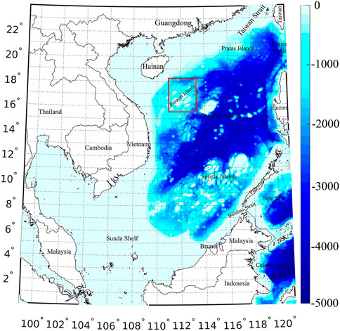
FIGURE 1. Study area and the associated bathymetry. The region enclosed in the red rectangle represents the surveyed area of airborne gravimetry over the Paracel Islands.
Several recently published high-degree GGMs, i.e., EGM2008, GECO, SGG-UGM-1, EIGEN-6C4, GOCO05c, XGM2016, XGM2019, and XGM2019e_2159 are investigated in this study. The reason for choosing the models above is that these models have relatively higher spatial resolutions and better accuracies compared to most of other GGMs, see the validation results against the globally distributed GPS/levelling data in http://icgem.gfz-potsdam.de/home. These models were computed by merging satellite gravimetric data and terrestrial and marine gravity data based on spherical harmonic functions. EGM2008 has a full expansion degree and order (d/o) of (2190/2159), which was computed by merging GRACE measurements with terrestrial gravity data on the land and altimetric gravity data in the ocean. Since no GOCE data have been incorporated for developing EGM2008, and the recently published GGMs were computed by combining GOCE data, which is supposed to improve the global gravity field in the frequency bands approximately from degree 30 to 220 in spherical harmonics representation (Gruber et al., 2014). As such, several recently released GOCE-based GGMs, i.e., the GECO (d/o 2190/2159) (Gilardoni et al., 2015), SGG-UGM-1 (d/o 2159/2159) (Liang et al., 2018), EIGEN-6C4 (d/o 2190/2159) (Förste et al., 2014), GOCO05c (Fecher et al., 2017), XGM2016 (Pail et al., 2018), XGM2019, and XGM2019e_2159 (Zingerle et al., 2019), are introduced. The detailed information with respect to the data sets used in these GGMs’ development is seen in Table 1.
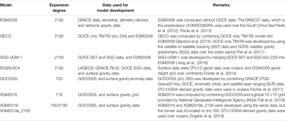
TABLE 1. Description of global geopotenital models.
An investigation of error degree variances offers an insight into the error spectra of a GGM, regarded as internal error estimates; and it supplies a rudimentary quality assessment (e.g., Pail et al., 2011). The cumulative geoid error of each GGM is calculated by using the estimated errors of Stokes’ coefficients of this model, and the equations we use can be seen in, e.g., Erol et al. (2020). Figure 2 shows the degree-wise accumulated geoid errors of different GGMs, demonstrates the error up to the maximal degree of each model. EGM2008 has relatively large error, which rises rapidly from degrees 30–220, and reaches ∼7.3 cm by the degree of 220 and then increases slowly to 8.2 cm by the maximal degree. Whereas, the accumulated geoid errors of the models that have similar expansion degrees, like GECO, SGG-UGM-1, EIGEN-6C4, and XGM2019e_2159 are reduced to ∼4.2, 2.7, 3.4, and 3.1 cm, respectively. The prominent error in EGM2008 at the frequency bands between degrees 30–220 is mainly due to the lack of GOCE data; and the other four models discussed above that developed with GOCE data have better qualities in this frequency bands, where GOCE data paly a dominant role in global gravity field recovery (e.g., Gruber et al., 2014). Moreover, the combination of updated altimetric gravity data may be the main reason that EIGEN-6C4/XGM2019e_2159 has smaller error than EGM2008 at short-wavelength bands. The comparisons of the GGMs that have lower truncated degrees, i.e., GOCO05C, XGM2016, and XGM2019, show that GOCO05C has the largest error, and its error increases dramatically after degree 170 and reaches 12.5 cm by the degree of 720. By comparison, the cumulative geoid error of XGM2016/XGM2019 reduces to ∼1.1/2.5 cm by its maximal degree.
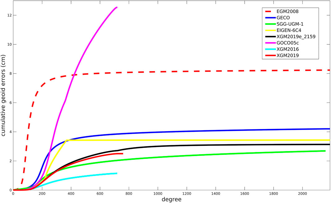
FIGURE 2. Cumulative geoid errors of different GGMs as a function of spherical expansion degree.
It is noteworthy that the correlation of errors of spherical harmonic coefficients is ignored when the (accumulated) error degree variances are computed, and the GGM’s error at a specific geographic location cannot be estimated. While, a more rigorous way for internal error estimate can be implemented through the error propagation by using the full error variance-covariance matrix of spherical harmonic coefficients of a GGM (Balmino, 2009). However, considering the limited accessibility of the full error variance-covariance matrices of the high-degree GGMs and the associated huge computation load, this method may be difficult to be implemented. Moreover, the polar gap problem exists in the GGMs that developed with GOCE data, which especially affects the qualities of zonal and near-zonal coefficients (Pail et al., 2011). In total, the error degree variances only supply a global mean of internal error and cannot be regarded as the realistic error estimate.
The First Geodetic Surveying Team of Ministry of Natural Resources of China conducted an airborne gravimetric survey in 2018, covered the Paracel Islands that located in the northwest SCS, see the enclosed area of the red rectangle in Figure 1. This area ranges from 15.5°N to 18.2°N latitude and 111.0°E to 113.3°E longitude. The airborne survey was implemented with a GT-2A gravimeter, which contained 87 flights in total to complete 61,594 line kilometers. It covered ∼270 km in east-west direction and ∼325 km in north-south direction, see Figure 3. The traverse lines were north-south oriented and spaced at 1 km, while the tie lines were east-west oriented and spaced at 5 km. The height of the flight ranged from 739 to 847 m above the mean sea level.
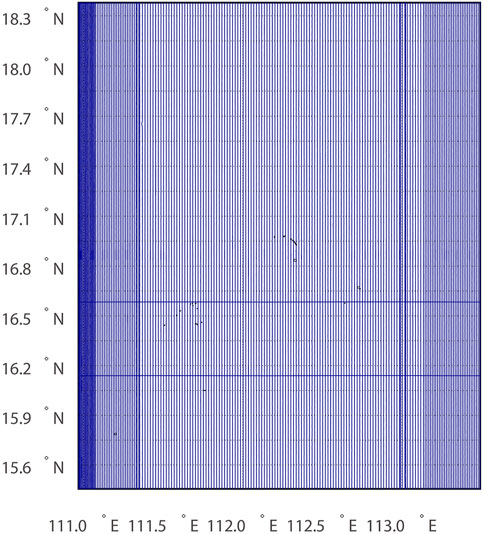
FIGURE 3. Flight lines of airborne gravimetric survey over the Paracel Islands.
The GT-2A gravimeter recorded the raw data at a frequency of 18.75 Hz, and the gravity data were calculated by subtracting the GPS-derived aircraft accelerations from the inertial accelerations, which were then corrected for the Eötvös effect and compensated for the off-level corrections. The derived gravity disturbances were filtered by a low pass filter with a cut-off frequency of 0.01 Hz to reduce the high-frequency noise, which were then resampled to 2 Hz corresponding to the epoch of GPS measurements. The spatial resolution of the derived airborne gravity disturbances after the filtering is ∼3 km. The airborne gravity data were then referenced to the China Geodetic Coordinate System 2000 (CGCS 2000), and the geodetic coordinates were referenced to the GRS80 reference ellipsoid. Seven repeat lines were conducted for quality control, and the overall standard deviation (SD) of the variations of repeat lines was ∼1.44 mGal. Moreover, the crossover measurements on transverse and tie lines offer an overview of the data quality, and the SD of the differences at crossovers was ∼1.54 mGal, showing in a good agreement with the statistics of the repeat lines. This airborne survey includes ∼1,854,900 point-wise data, which haven’t been used for global/regional gravity field model development.
The marine gravity anomalies are retrieved from the National Geophysical Data Center (NGDC) in the National Centers for environmental information (NCEI), where worldwide shipborne gravity data collected during the marine cruises from 1939 to present are available. The original gravity data suffer from the instrument errors, navigational errors, and biases stemming from the inconsistencies among different height systems as well as other systematic errors (Denker and Roland, 2005; Wu et al., 2017a). DTU17GRA is introduced to ensure the quality of the shipborne data. This model combined the 25 years of satellite altimetry data and included the recent altimeter data from Jason-1, CryoSat-2, and SARAL/Altika. The comparison with independent gravity data showed that DTU17GRA had improved precision compared with the previous versions developed at DTU space (Andersen and Knudsen, 2019). The erroneous shipborne gravity data from the NGDC are first removed through a 3-sigma rule, i.e., data are identified as blunders if the difference between the shipborne gravity data and DTU17GRA-derived value is larger than three times of the SD of all the differences. Since the shipborne gravity data originated from various epochs and systematic errors were likely to exist, we apply a crossover adjustment to reduce the systematic errors. The duplicate data are then removed and we assume a constant bias for each track. It is noteworthy that not all the systematic errors can be estimated due to the lack of track information for some cruises. The SD of the differences at the crossovers is estimated as 8.4 mGal, which is slightly smaller than the SD of the differences between DTU17GRA-derived values and shipborne gravity data before the crossover adjustment, with a value of ∼9.0 mGal.
The performances of different GGMs are investigated in MDT and geostrophic velocities recovery, where an existing synthetic MDT and three ocean models are introduced for comparison. The synthetic MDT is called CNES-CLS13MDT, and it covers the period of 1993–2012 at a resolution ∼0.25° (∼30 km). This model was estimated by using the CNES-CLS11 mean sea surface (MSS) data and EGM-DIR R4 (a satellite-only GGM) as the raw solution, which was then enhanced by in situ data to recover unresolved small-scale signals (Rio et al., 2011). Three ocean models, i.e., the Simple Ocean Data Assimilation, version 3 (SODA3) (Carton et al., 2018), the ocean reanalysis product of the European Centre for Medium-Range Weather Forecasts, version 5 (ECMWF ORAS5) (Zuo et al., 2017), and the Ocean Circulation and Climate Advanced Modeling Project (OCCAM) (Fox and Haines, 2003), are ocean reanalysis products provided with the field of dynamic topography. SODA3 was developed by ocean reanalysis with enhancements to model resolution, observation, forcing data, and the addition of active sea ice. This model maps the ocean state from 1980 to 2017, and it has a 0.25° horizontal resolution. ORAS5 is a recently released ocean reanalysis product from the ECMWF, which was developed from Ocean ReAnalysis Pilot 5 (Zuo et al., 2017) using the same ocean and sea ice model and data assimilation method. ORAS5 has a horizontal resolution of 0.25°, and it supplies monthly data from 1979 to 2018. The OCCAM MDT (0.5° horizontal resolution) maps the ocean state from 1993 to 2004, and was developed by using a hydrodynamic model forced with wind stresses from the ECMWF, hydrographic data, and surface temperature (Fox and Haines, 2003).
The maximal expansion degrees of EGM2008, EIGEN-6C4, GECO, SGG-UGM-1, and XGM2019e_2159 are higher than those of XGM2016, XGM2019, and GOCO05c. For the sake of comparison, the computations with the models that have higher expansion degrees are not only carried out up to the maximal degrees but also truncate to degree 720. Table 2 shows the statistics of the differences between the airborne gravity disturbances and the quantities synthesized from different GGMs at the flight altitude. The statistics derived from XGM2016, GOCO05c, and GGMs that truncated to degree 720 are very close, and the SD values of the misfits against the airborne data are ∼9.0 mGal. The models that truncate to degree 720 cannot recover the contents with the wavelengths shorter than ∼30.4 km; and consequently, large inconsistencies against the airborne data are observed. Figure 4 demonstrates the discrepancies between different GGMs and the airborne data (several representative models are displayed), and most significant discrepancies concentrate at regions close to islands in the Paracel Islands (see Figure 1). The main reason may be due to the degraded quality of altimetry data used in developing these GGMs, while the airborne survey does not suffer from the problem like waveform contamination near coast/island and provides accurate observations.
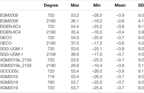
TABLE 2. Statistics of the differences between the airborne gravity disturbances and quantities synthesized from different GGMs over the Paracel Islands (units: mGal).
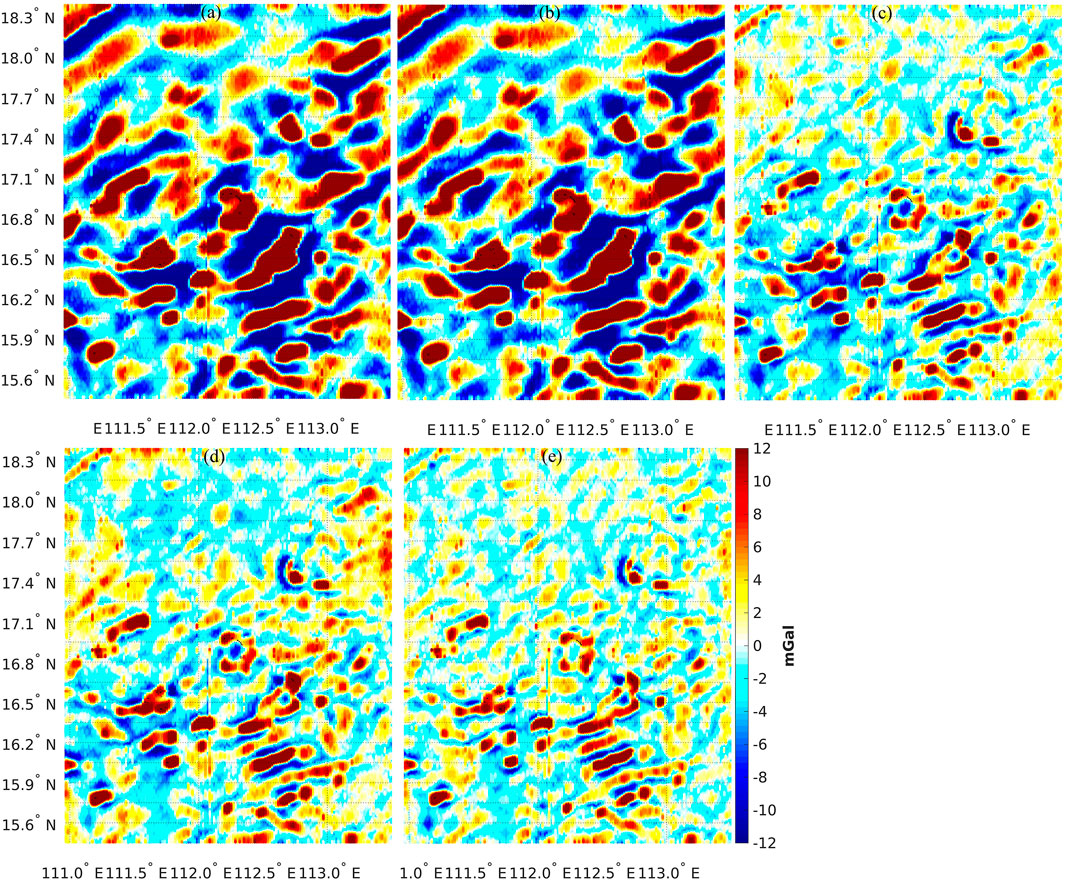
FIGURE 4. Differences between the airborne gravity disturbances and quantities synthesized from (A) GOCO05c (d/o 720), (B) XGM2019 (d/o 760), (C) EGM2008 (d/o 2190), (D) EIGEN-6C4 (d/o 2190), and (E) XGM2019e_2159 (d/o 2190) over Paracel Islands.
The expansions of the GGMs that have higher expansion degrees to the maximal degrees recover more small-scale signals and significantly reduce the discrepancies against the airborne data; and the SD values of the misfits are reduced by a magnitude of ∼5 mGal, compared to results derived from the models truncated to degree 720, see Table 2. However, these GGMs, i.e., with a full expansion degree of 2190 (2159), sample the gravity field at a resolution of ∼10 km, which is still inferior to the mean resolution of airborne data (∼3 km); and the high-frequency signals that have the wavelengths shorter than 10 km are missed in these models. As a result, the differences between these GGMs and the airborne data demonstrate as high-frequency features.
The mutual comparisons show that EGM2008, GECO, and SGG-UGM-1 have comparable qualities, with a SD value of ∼4.0 mGal. GECO/SGG-UGM-1 that computed based on EGM2008 but additionally with GOCE data does not demonstrate better result than EGM2008. The possible reason is that GOCE data mainly contribute to long-wavelength bands (degrees 30–220), and the effects introduced by GOCE data are not prominent in terms of gravity disturbances since they are dominated by local short-wavelength features. EIGEN-6C4 does not show improved performance compared to EGM2008/GECO/SGG-UGM-1, although EIGEN-6C4 was computed based on an updated altimetric gravity model (DTU12 data) versus DNSC07GRA that used in developing EGM2008 (Andersen, 2010). Whereas, XGM2019e_2159 has relative high quality and the SD of the misfits reduces to ∼3.1 mGal; and the discrepancies against the airborne data reduce dramatically close to islands, see Figure 4E. The better fit of XGM2019e_2159 with the airborne data is largely attributed to the use of updated altimetric gravity data in model development, i.e., DTU13GRA; and DTU13GRA has improved quality compared to DNSC07GRA that was used in computing EGM2008 (Andersen et al., 2013). Thus, the incorporation of the updated altimetric gravity data may be the main reason that XGM2019e_2159 has better quality than the other models that have similar expansion degrees.
The SD of the differences between the shipborne gravity anomalies retrieved from the NGDC and the quantities synthesized from different GGMs that have the maximal expansion degree of 2190 (2159) are ∼9.4 mGal, see the statistics in Table 3 and Figure 5. The qualities of these GGMs cannot be discriminated; and this is probably due to the limited accuracy of the shipborne gravity data, the quality of which may be questionable since some of them were collected decades ago without GPS navigation. Considering the restricted distribution of the airborne survey and suspicious quality of the shipborne data as well as the data gaps of marine surveys in the western and northern SCS, the validation against local airborne/shipborne data cannot be treated as the representative error estimate of a GGM over the SCS.
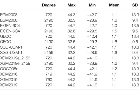
TABLE 3. Statistics of the differences between the shipborne gravity anomalies retrieved from NGDC and quantities synthesized from different GGMs over South China Sea.
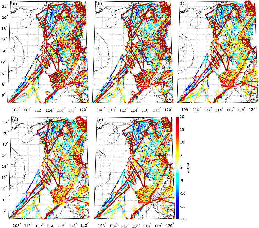
FIGURE 5. Differences between shipborne gravity anomalies retrieved from NGDC and quantities synthesized from (A) GOCO05c (d/o 720), (B) XGM2019 (d/o 760), (C) EGM2008 (d/o 2190), (D) EIGEN-6C4 (d/o 2190), and (E) XGM2019e_2159 (d/o 2190) over South China Sea.
Before computing the geodetic MDT, we study the error information of different versions of MSS in order to choose an appropriate MSS. The interpolation errors of two recently released models, i.e., DTU15MSS (Andersen et al., 2016) and DTU18MSS (Andersen et al., 2018), are studied. Figure 6 shows the errors of these models, and the root mean square (RMS) of errors of DTU15MSS and DTU18MSS are 1.95 and 1.78 cm, respectively, which indicate that DTU18MSS has better quality. DTU18MSS shows improved quality along the southern coast of Guangdong in China, the eastern coast of Vietnam and Malaysia, and the western coast of Luzon and coastal areas over Philippines. The reason that DTU18MSS outperforms DTU15MSS is mainly due to the incorporation of more high-quality altimeter data and the use of improved data pre-processing methods (Andersen et al., 2018).

FIGURE 6. Interpolation errors of (A) DTU15MSS, and (B) DTU18MSS over South China Sea.
MDT determined through a geodetic approach illustrates the departure of the MSS from the geoid/quasi-geoid (Bingham et al., 2011a, 2014; Griesel et al., 2012). The raw geodetic MDT is computed as the difference between DTU18MSS and quasi-geoid computed from a GGM expanded to its maximal degree. For cross validation, CNES-CLS13MDT, SODA3 MDT, ORAS5 MDT, and OCCAM MDT are introduced, where the former three models have a resolution of 0.25°, while the resolution of OCCAM is 0.5°. The raw geodetic MDT contains small-scale contents that cannot be resolved in synthetic/ocean data, and we apply a Gaussian filter with a correlation length of 30 km to the raw geodetic MDT for ensuring a spectrally consistent comparison. Different MDTs are referenced to various time periods, and we use the method suggested by Bingham and Haines (2006) to unify the time period, where all the models are adjusted to the geodetic MDT time period (1993–2018). The AVISO altimetric sea level anomaly (SLA) is used to standardize all the MDTs to the required period (e.g., Rio et al., 2011). The CNES-CLS13MDT is adjusted to the 1993–2018 period computed as CNES-CLS13MDT (93–2018) = CNES-CLS13MDT (93–2012) + MSLA (93–2018) − MSLA (93–2012), and MSLA denotes the mean value of SLA over a specific time period. For OCCAM MDT, a similar method is used to adjust its period to 1993–2018. For SODA3, we first compute the mean SODA MDT by averaging the monthly data from 1993 to 2017, which is then adjusted to 1993–2018 by using the SLA data. For ORAS5, the associated MDT is retrieved by averaging the monthly data from 1993 to 2018.
Different MDTs generally have analogous structures, vary in a range of ∼0.5 m, see Figure 7, where the maximum value up to 0.9 m appears around the western coast of Cambodia; while, the minimum value, roughly 0.5 m, occurs in the northern SCS. However, prominent discrepancies between the geodetic MDTs and synthetic/ocean models are observed, particularly in the northern SCS, by a magnitude up to 10 cm. The behaviors of MDTs computed from different GGMs are heterogeneous, where the signals derived from EGM2008, GECO, SGG-UGM-1, and EIGEN-6C4 have relatively significant oscillations over the southern part, compared to ones calculated from the other four GGMs. Moreover, the magnitudes of MDT signals of different synthetic/ocean models are not consistent, where CNES-CLS13MDT has smaller values over the northern SCS, while ORAS5 has larger values around the Luzon Strait.
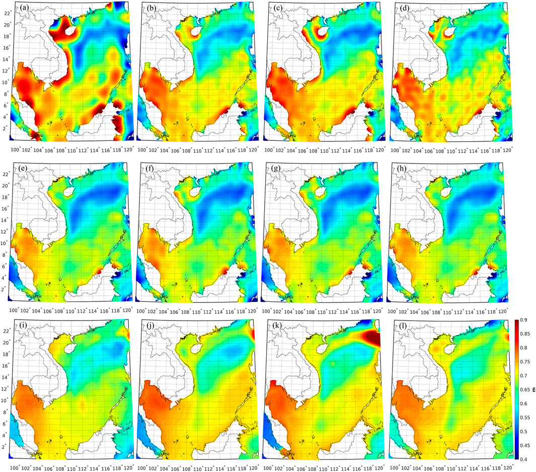
FIGURE 7. Geodetic MDT calculated from (A) EGM2008, (B) GECO, (C) SGG-UGM-1, (D) EIGEN-6C4, (E) XGM2019_2159, (F) GOCO05c, (G) XGM2016, and (H) XGM2019; and existing synthetic/ocean models, (I) CNES-CLS13MDT, (J) SODA, (K) ORAS5, and (L) OCCAM.
The extreme values exist in the geodetic MDTs along the coast of Hainan, eastern coast of Vietnam, and western coast of Brunei and Malaysia. These values are identified as outliers, due to the uncorrected errors in the MSS model and errors in the quasi-geoid (Hipkin et al., 2004; Wu et al., 2017b; Wu et al., 2019). The remaining errors in the MSS model are mainly due to the orbit errors and errors in various range corrections (e.g., Andersen and Knudsen, 2009). However, these errors have been significantly reduced with the combination of recent altimeter data, even over coastal areas, see Figure 6. Whereas, the quasi-geoid over coastal regions suffers from the scarcity of surveyed gravimetric data, the degraded quality of altimetric gravity data, and the uncorrected biases/tilts among different data sets that used in computing the quasi-geoid (Huang, 2017; Wu et al., 2019). The EGM2008 commission errors, composed of the low-degree errors estimated by using a satellite-only model through error propagation and high-degree ones computed through an integral formula using surface gravity data (Pavlis et al., 2012), are seen in Appendix A. These errors reach decimeter level along the coastal regions over the SCS, suggesting that the computed geodetic MDTs prominently suffer from the errors in the associated GGMs, even though the application of filtering suppresses the high-frequency noises.
CNES-CLS13MDT and three ocean models are used as control data for model assessment; however, the lack of formal error of synthetic/ocean model remains an obstacle for deriving reliable results through an individual model. Thus, we not only provide the results computed from each synthetic/ocean model, but also give the statistics derived from the comparisons with the mean value of all synthetic/ocean models, which provide sufficient independence and redundancy to allow more robust comparison. Figure 8 demonstrates the discrepancies between the MDTs computed from different GGMs and the mean of all synthetic/ocean data. The MDT derived from EGM2008 has the largest oscillations, and the maximum/minimum value is 17.9/-19.7 cm, with a SD of 6.4 cm, see Table 4. The significant long-wavelength errors are observed in the MDT derived from EGM2008, by a magnitude greater than 3 cm, and this is probably due to the lack of GOCE data in the computation of EGM2008. The long-wavelength errors are consequently reduced when the GGMs computed with GOCE data are applied, for instance, see the MDT derived from GECO/XGM2019e_2159 in Figure 8. Moreover, the coastal problem is extremely prominent in the MDT computed from EGM2008, especially around the coast of Hainan, Vietnam, Malaysia, and Brunei, where the errors reach a magnitude greater than 10 cm. This is attributed to the use of relatively low quality of altimetric gravity data in computing EGM2008 and the data voids occurred close to coast/island when EGM2008 was computed. In contrast, the MDT derived from SGG-UGM-1/GECO shows less variations and improved consistencies comparing with the synthetic/ocean data, and the SD of the misfits reduces to 3.3/4.1 cm. The incorporation of GOCE data is the main reason that these two MDTs show improved qualities at long-wavelength bands than the one computed from EGM2008. Moreover, the application of GECO/SGG-UGM-1 substantially reduces the errors of the associated MDT over coastal regions, for instance, along the coast of Hainan and Vietnam. The mutual comparison shows that the MDT derived from GECO has better quality than that computed from SGG-UGM-1, where the different methods for model development and data merging/assimilation approaches may account for these differences. The MDT derived from EIGEN-6C4 has comparable quality as that derived from GECO; however, the errors in the MDT model derived from EIGEN-6C4 are reduced over coastal regions, compared to the one derived from GECO/SGG-UGM-1. EIGEN-6C4 was computed by combining GRACE, GOCE, and EGM2008 data, but it included DTU12 geoid data over oceans; and this may be the main reason that EIGEN-6C4 has better performance in coastal MDT computation than EGM2008/GECO/SGG-UGM-1. We also notice that significant small-scale contents propagate into the MDT computed from EIGEN-6C4, particularly in the southern SCS, indicating that the use of the Gaussian filter may not be an optimal way to make a spectrally consistent fusion of the MSS and the quasi-geoid. The comparisons with local shipborne/airborne data show that these GGMs discussed above have comparable qualities; moreover, these models typically show comparable accuracies when validated against GPS/levelling data, e.g., see Featherstone et al. (2018) and Wu et al. (2018). However, this is not true when comparing with the synthetic/ocean data, where the qualities of these models can be discriminated.
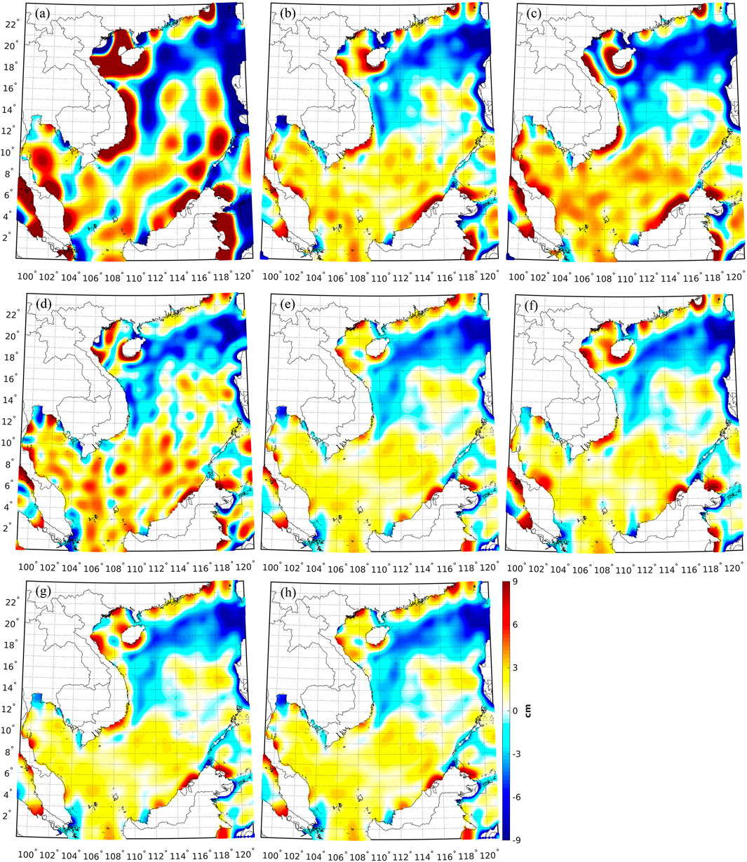
FIGURE 8. Differences between the MDT computed from (A) EGM2008, (B) GECO, (C) SGG-UGM-1, (D) EIGEN-6C4, (E) XGM2019e_2159, (F) GOCO05c, (G) XGM2016, (H) XGM2019 and mean value of all synthetic/ocean models.
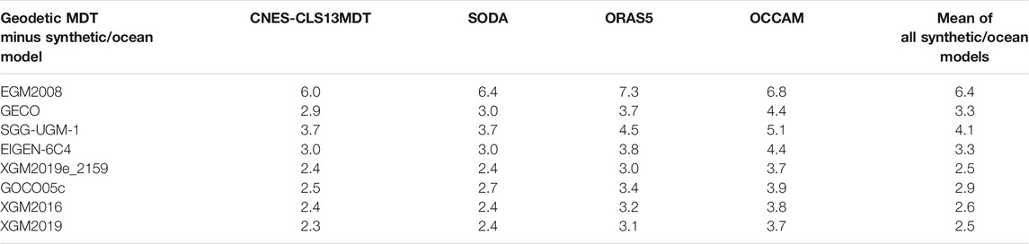
TABLE 4. The standard deviation of the differences between the MDTs derived from different GGMs and synthetic/ocean model.
The use of XGM2019e_2159 leads to a more consistent MDT with the synthetic/ocean data, which demonstrates less variations compared to the MDTs derived from the GGMs described above. The SD of the misfits between the MDT calculated from XGM2019e_2159 and the synthetic/ocean data is ∼2.5 cm, with a reduction of ∼0.8/0.8/1.6/3.9 cm, compared to the MDT computed from GECO/EIGEN-6C4/SGG-UGM-1/EGM2008. This is mainly attributed to the combination of recent satellite gravimetry and altimetry data in computing XGM2019e_2159, which combined a recently released GRACE/GOCE satellite-only model (GOCO06s) at long wavelength and DTU13GRA data at short-wavelength. DTU13GRA has better quality than the previous versions, e.g., DTU10GRA and DNSC07GRA, and the quasi-geoid calculated from XGM2019e_2159 was improved accordingly. This result is commensurate with the validation results against the airborne gravity data over the Paracel Islands, where XGM2019e_2159 has relatively high quality.
For the MDTs computed with the GGMs that have lower expansion degrees, the SD of the misfits between the MDT modeled from GOCO05c and the synthetic/ocean data is ∼2.9 cm; while, for the MDT computed from XGM2016/XGM2019, this value is slightly better, by a magnitude of 0.3/0.4 cm XGM2016 was developed using the same methodology as GOCO05c, but the input surface data were different, where GOCO05c used DTU13GRA data, while XGM2016 combined NGA gridded data at oceans. The MDTs derived from XGM2019 and XGM2019e_2159 have almost identical features, since XGM2019 was computed using the same input data sets and modeling method as XGM2019e_2159, but truncated to degree 760.
The comparison of each synthetic/ocean model and the geodetic MDTs derived from different GGMs show that CNES-CLS13MDT/SODA has smaller discrepancies against the geodetic MDTs, compared to ORAS5/OCCAM. This indicates that geodetic MDT may be used for synthetic/ocean model assessment, particularly in the regions lack of in situ data (e.g., buoys and hydrological profiles). However, it should be emphasized that these results are rudimentary ones since the error information of the ocean models is not available and no in situ data have been for evaluating the synthetic/ocean models and geodetic MDTs in this study.
In addition, the geodetic MDTs’ characteristics along the zonal/meridian profile are investigated. Figure 9A shows the zonal mean of the misfits between different geodetic MDTs and the mean of all synthetic/ocean data. The MDT derived from EGM2008 demonstrates strong oscillations, and the spike-like errors appear, by a magnitude up to 5 cm. The MDT derived from SGG-UGM-1/EIGEN-6C4 has slightly better performance; however, the spikes are still prominent. For instance, the MDT computed from SGG-UGM-1 has strong variations from 18°N to 21°N, where this profile passes through the regions around Hainan in China. This corresponds to the result that the MDT derived from SGG-UGM-1 has large errors around Hainan because of the coastal problem. In contrast, the MDTs computed from the other GGMs show improved qualities, and almost no apparent spikes are found. The MDT derived from XGM2019e_2159/XGM2019 has relatively small variations, and the discrepancies against the synthetic/ocean data are within 3 cm. The misfits between the geodetic MDTs and the ocean data are reduced along the meridian profile compared to the ones derived from the zonal profile, see Figure 9B. This is mainly due to the configuration of satellite orbits, which affects the error structures of the GGM-derived quantities. As the orbit of GRACE/GOCE is almost south-north oriented, the along-track data sampling is much denser than that in the across-track direction; and consequently, larger errors were found in east-west direction than in north-south direction (Balmino, 2009; Bingham et al., 2011b). Similar validation results are concluded along the meridian profile as ones derived from the zonal profile, where the signal calculated from XGM2019e_2159/XGM2019 has relatively high quality.
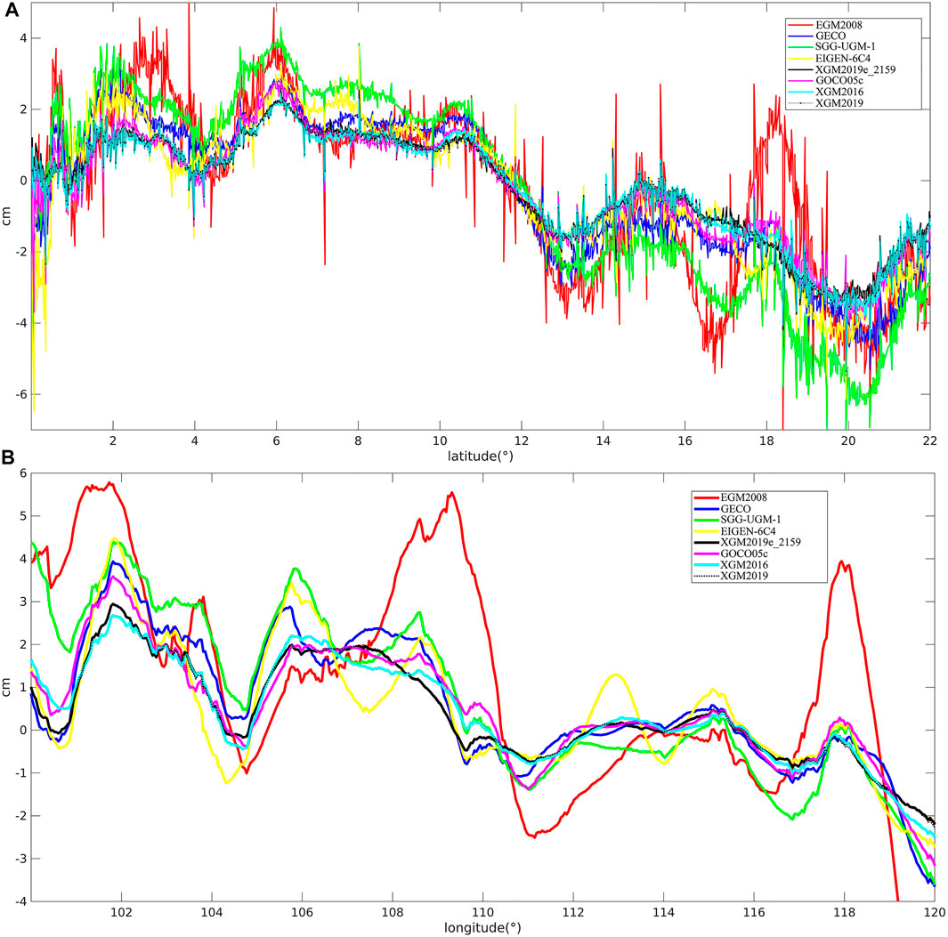
FIGURE 9. The zonal (A) and meridian (B) mean of the misfits between the MDTs derived from different GGMs and mean of all synthetic/ocean models.
The performances of different GGMs are further assessed in terms of geostrophic velocities. Apart from the synthetic/ocean data shown in Existing MDTs and Ocean Models, another reanalysis data set derived from an ocean data assimilation system in Asia, the Indian Ocean, and the western Pacific Ocean (AIPO), known as AIPOcean (Yan et al., 2015), is introduced. AIPOcean data was developed based on the ensemble optimal interpolation (EnOI) method, where various types of observations including the AVISO altimetric SLA, satellite-sensed sea surface temperature, and in situ temperature and salinity profiles, were assimilated. AIPOcean data contains the daily averaged ocean current field from January 1, 1993 to December 31, 2006, with a horizontal resolution of 0.25°. The comparisons with independent observations and other reanalysis products show that the quality of AIPOcean data was well controlled, which provided the realistic structures of the ocean state in AIPO (Yan et al., 2015).
AIPOcean data map the ocean currents from 1993 to 2006 with a horizontal resolution of 0.25°, and the synthetic/geodetic MDT is adjusted to this time period based on AVISO SLA data, and then the geostrophic velocities are computed. Whereas, the surface currents provided in the ocean models are retrieved and averaged to map the signals over the 1993–2006 time period. Figure 10 shows the zonal velocities computed from the geodetic MDTs and the synthetic/ocean data, which generally reconstruct the real surface circulation over the SCS. For instance, the blue strip-like features over the northern of SCS that passes through the southern of Hainan is the South China Sea Warm Current (SCSWC), playing a key role in distribution of mass, energy, and heat balances over the northern SCS (Hsueh and Zhong, 2004; Chiang et al., 2008; Yang et al., 2008). Moreover, the yellow/red signals along the Guangdong coast are known as Guangdong Coastal Current (GCC) (Hu et al., 2000; Gu et al., 2012). However, the structures of GCC are not identical in different models. For example, the intensity of GCC in CNES-CLS13MDT/SODA is not as strong as that in ORAS5/OCCAM/AIPO.
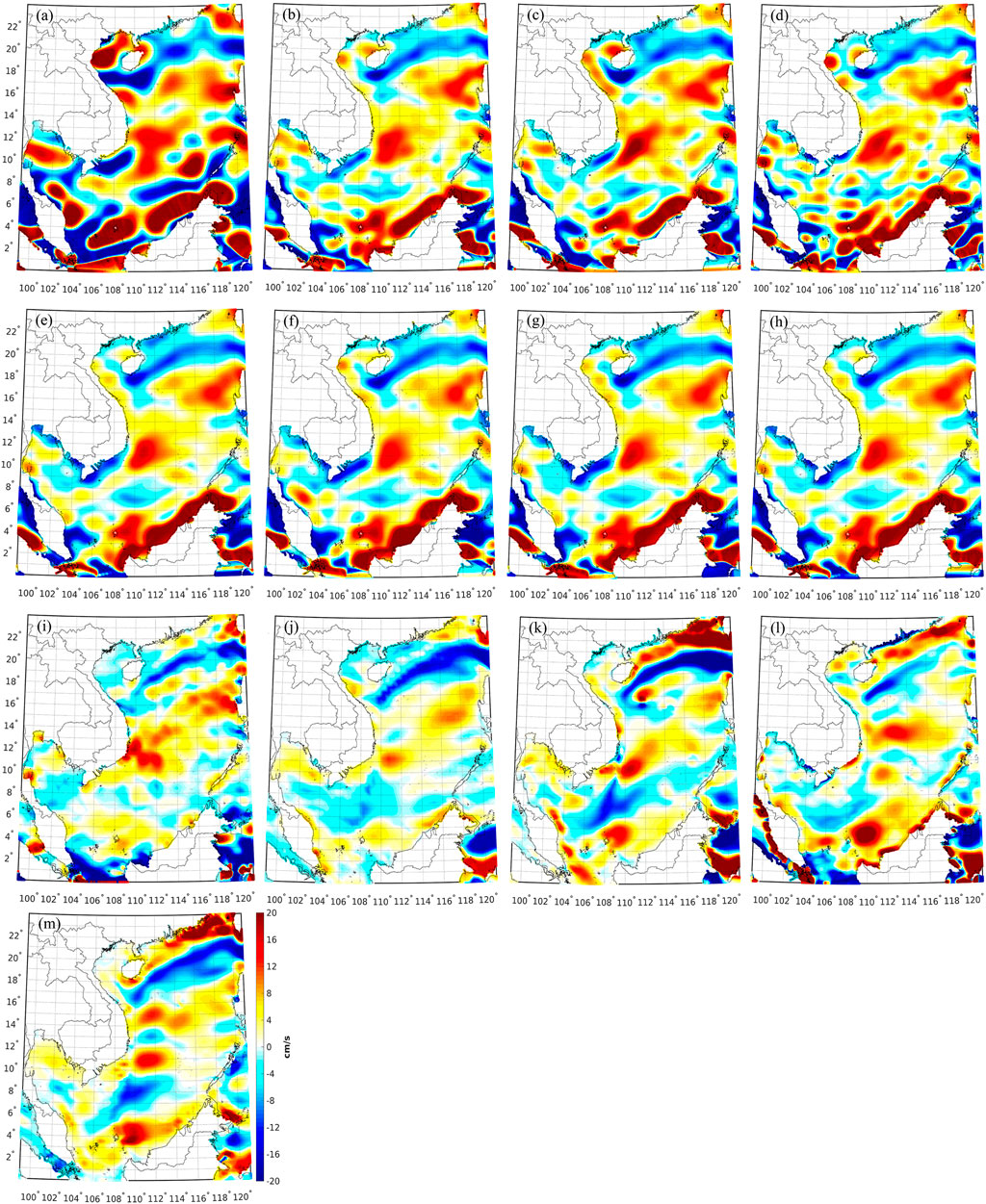
FIGURE 10. Zonal geostrophic velocities derived from the MDT computed from (A) EGM2008, (B) GECO, (C) SGG-UGM-1, (D) EIGEN-6C4, (E) XGM2019_2159, (F) GOCO05c, (G) XGM2016, (H) XGM2019, (I) CNES-CLS13MDT; and zonal velocities retrieved from (J) SODA, (K) ORAS5, (L) OCCAM, and (M) AIPO.
The detailed features of the zonal velocities derived from the geodetic MDTs and ocean models are heterogeneous. For signals computed from the geodetic MDTs, more scattered structures are observed in the values computed from the MDT derived from EGM2008, displaying as prominent long-wavelength patterns, especially in the southern SCS. However, these large-scale contents cannot be treated as real ocean circulation signals, since the long-wavelength contents of EGM2008 are questionable due to the lack of GOCE data. By comparison, the velocities computed from the MDTs derived from other GGMs show less variations and smoother patterns. It is noticeable that a high-degree GGM suffers from the coastal problem, where the errors in the associated MDT are magnified in the computation of geostrophic velocities, since the gradients of MDT are used to compute the geostrophic velocities. However, the coastal problem may be mitigated by using the recent altimeter data (Ophaug et al., 2015; Idžanović et al., 2017) and airborne gravimetric survey (Hwang et al., 2006; Wu et al., 2019).
CNES-CLS13MDT and SODA demonstrate smoother structures than other ocean models over the southern SCS, and significant small-scale structures are observed in CNES-CLS13MDT over the northern part. While, ORAS5, OCCAM, and AIPO have relatively intense features over the Guangdong coast, compared to CNES-CLS13MDT/SODA. Different methods and input data for model development are the main reasons for these differences. For example, CNES-CLS13MDT is a synthetic model, estimated through a geodetic method as a raw solution, which was then enhanced by in situ data to recover the small-scale contents. While, the ocean models are the ocean reanalysis products developed by combining ocean state data, hydrographic data, surface temperature, and so on.
Figure 11 demonstrates the discrepancies between the zonal geostrophic velocities computed from different geodetic MDTs and the mean of all synthetic/ocean data, and the associated statistics are given in Table 5. The performances of the velocities computed from different geodetic MDTs are heterogeneous. The zonal velocities derived from the MDT modeled with EGM2008 have the largest oscillations, where the SD of the inconsistencies against the mean of synthetic/ocean data is 11.1 cm/s. The prominent discrepancies occur over the southern of SCS and along the coast of Vietnam, Malaysia and Philippines, by a magnitude up to 20 cm/s. The comparisons of EGM2008 and other models that have similar resolutions, i.e., GECO, SGG-UGM-1, EIGEN-6C4, and XGM2019e_2159, show that the zonal velocities computed from the MDTs modeled with these four models have improved qualities, and the SD values of the misfits reduce to 7.1–7.9 cm/s. The errors of the geostrophic velocities computed from these four models are significantly reduced over coastal regions, especially in the southern coast of Guangdong, north-eastern and south-eastern coast of Vietnam, western coast of Malaysia and Philippines. The mutual comparisons show that the zonal velocities derived from the MDT computed from GECO/XGM2019e_2159 have better qualities than the ones computed from the MDT modeled with SGG-UGM-1/EIGEN-6C4. This is not consistent with the results derived from the MDT comparison, where the MDT computed from GECO has lower quality than the one derived from XGM2019e_2159, but has comparable quality with the MDT derived from EIGEN-6C4. The SD of the misfits of the zonal velocities derived from the MDTs modeled with GOCO05c, XGM2016, and XGM2019 are 7.4, 7.4, and 7.1 cm/s, respectively, where the velocities derived from the MDT modeled with XGM2019 show better performances.
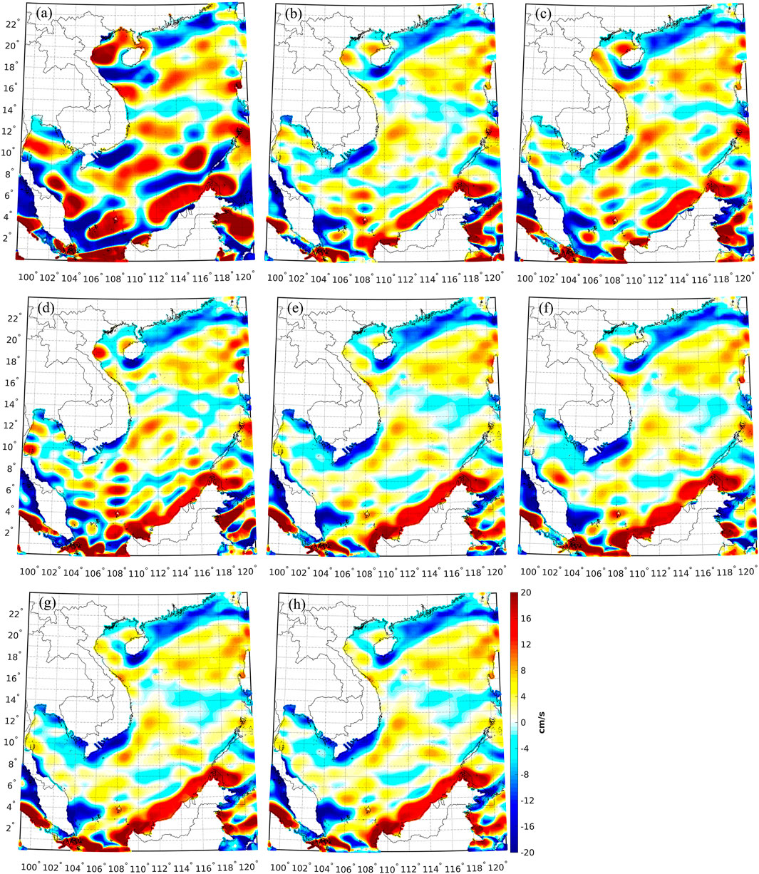
FIGURE 11. Differences between the zonal velocities computed from the MDT computed from (A) EGM2008, (B) GECO, (C) SGG-UGM-1, (D) EIGEN-6C4, (E) XGM2019e_2159, (F) GOCO05c, (G) XGM2016, (H) XGM2019 and the mean of the zonal velocities derived from all synthetic/ocean data.
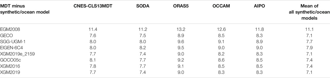
TABLE 5. The standard deviation of the differences between the zonal velocities synthesized from the MDTs modeled from different GGMs and those derived from synthetic/ocean data.
The meridian velocities synthesized from the geodetic MDTs and the synthetic/ocean data are seen in Figure 12, which represent the north-southward ocean circulation of SCS. For instance, a southward along-shelf current is seen along the coast of Vietnam, see the blue stripe-like features, which is mainly caused by local monsoon system (Hu et al., 2000; Chen et al., 2012). In addition, the red signals cross the Luzon Strait are line with the Kuroshio intrusion, e.g., see Hu et al. (2000) and Xue et al. (2004). The comparison results are seen in Figure 13; Table 6, where the velocities computed from the MDT modeled with EGM2008 have the worst performances, the SD of the misfits against the ocean data reaches 12.3 cm/s. Whereas, the SD values reduce to 7.6, 8.0, 8.6, and 6.8 cm/s, respectively, when the velocities derived from the MDTs modeled with GECO, SGG-UGM-1, EIGEN-6C4, and XGM2019e_2159 are assessed. The SD of the misfits of the meridian velocities derived from the MDTs modeled with GOCO05c, XGM2016, and XGM2019 is 7.7, 7.3, and 6.9 cm/s, respectively, where the signals derived from the MDT modeled with XGM2019 also have better performances.
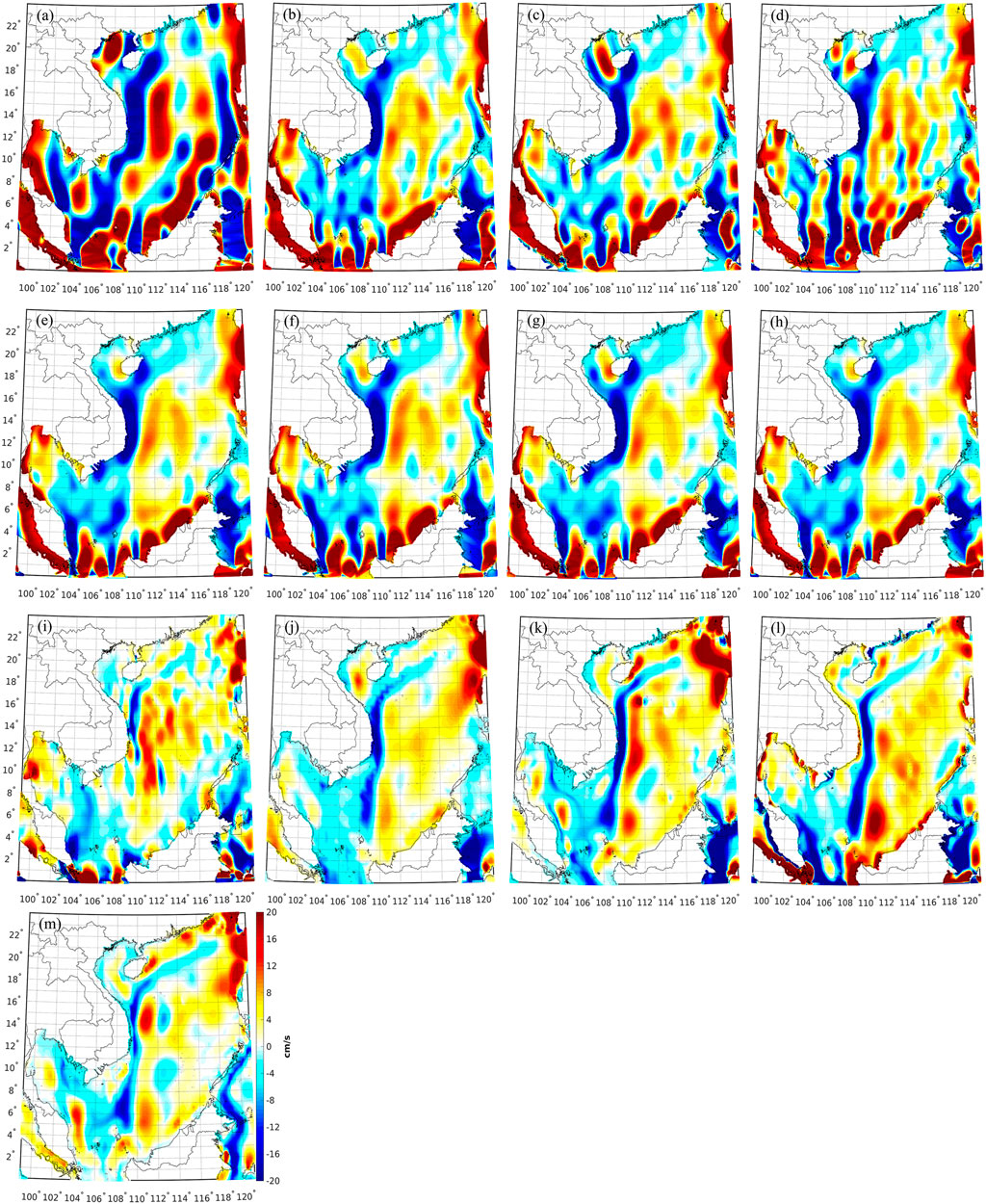
FIGURE 12. Meridian geostrophic velocities computed from the MDT derived from (A) EGM2008, (B) GECO, (C) SGG-UGM-1, (D) EIGEN-6C4, (E) XGM2019_2159, (F) GOCO05c, (G) XGM2016, (H) XGM2019, (I) CNES-CLS13MDT; and meridian velocities retrieved from (J) SODA, (K) ORAS5, (L) OCCAM, and (M) AIPO.
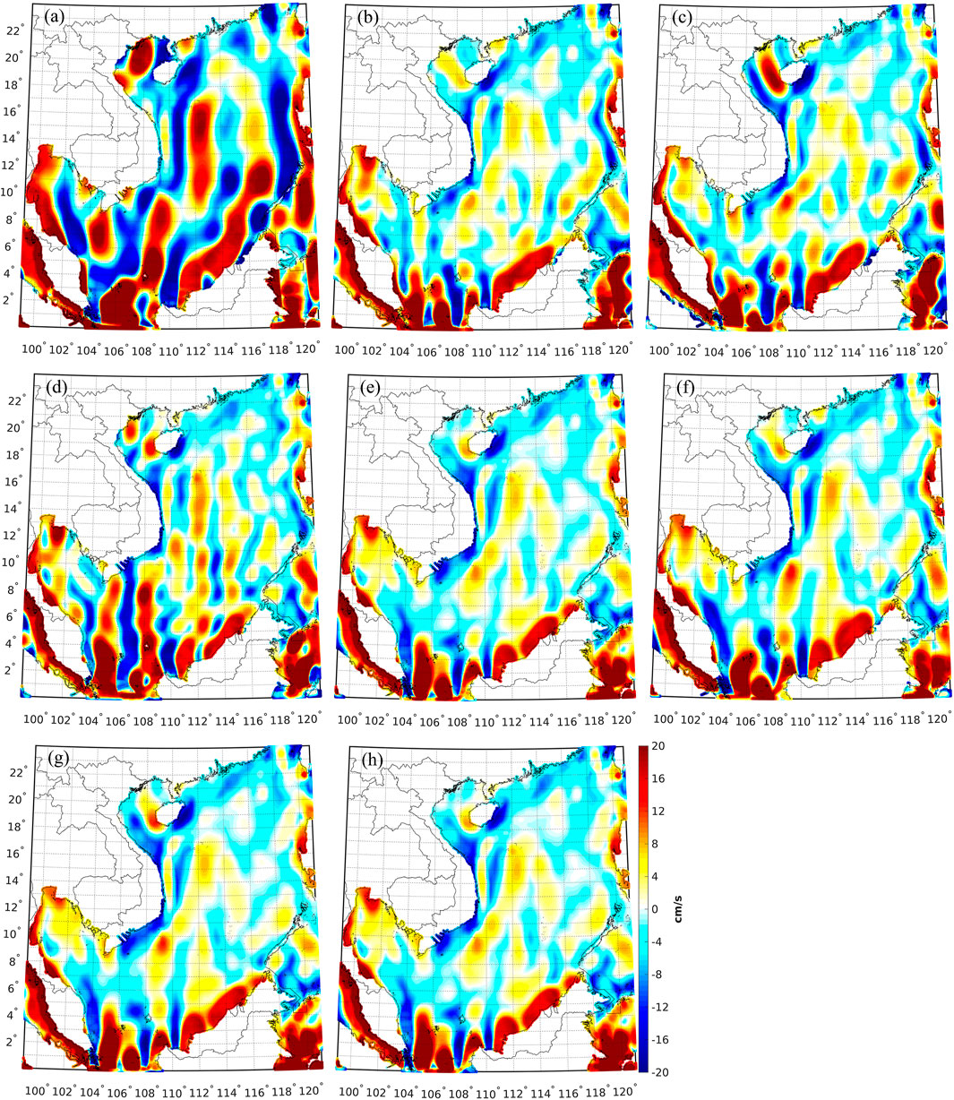
FIGURE 13. Differences between the meridian velocities computed from the MDT derived from (A) EGM2008, (B) GECO, (C) SGG-UGM-1, (D) EIGEN-6C4, (E) XGM2019e_2159, (F) GOCO05c, (G) XGM2016, (H) XGM2019 and the mean of the meridian velocities derived from all synthetic/ocean data.
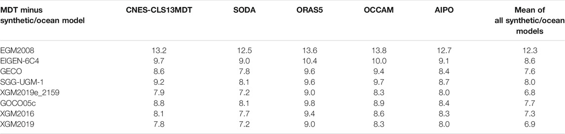
TABLE 6. The standard deviation of the differences between the meridian velocities synthesized from the MDTs modeled from different GGMs and those derived from synthetic/ocean models.
The wide range of applications of the global geopotential models in ocean science emphasizes the importance for model assessment. We assess the qualities of the recently released high-degree GGMs over the South China Sea, where local airborne/shipborne gravity data and independent synthetic/ocean reanalysis data are served as the control data.
A comparison with a high resolution (∼3 km) airborne gravimetric survey over the Paracel Islands shows that XGM2019e_2159 has relatively high quality, and the SD of the misfits against the airborne gravity data is ∼3.1 mGal. The SD values increase to ∼4.0 mGal when EGM2008, GECO, SGG-UGM-1, and EIGEN-6C4 are validated; however, the qualities of these models cannot be discriminated. Whereas, the comparisons with the shipborne gravity data that retrieved from the NGDC cannot discriminate the qualities of different GGMs that have the same expansion degree, due to the limited data precision.
The assessments with the synthetic/ocean data show that the qualities of the values derived from different GGMs are heterogeneous. The MDT computed from XGM2019e_2159 has relatively high quality, showing in an agreement with the validation results against the airborne gravity data. The SD of the differences between the MDT modeled with XGM2019e_2159 and the mean of all synthetic/ocean data is ∼2.5 cm; and this value changes to 7.1 cm/s (6.8 cm/s) when the associated zonal (meridian) velocities are assessed. The assessments of the quantities modeled with EIGEN-6C4, GECO, SGG-UGM-1, GOCO05c, and XGM2016 show that they have deteriorated qualities than the ones derived from XGM2019e_2159, with a reduction of approximately 0.1–1.6 cm in terms of MDT, and of 0.3–1.8 cm/s in terms of geostrophic velocities. The values derived from EGM2008 demonstrate the worst performances, which is reduced by 3.9 cm when the MDT is assessed, and by 4.0 cm/s (5.5 cm/s) when the zonal (meridian) velocities are assessed, compared to the results derived from XGM2019e_2159. Moreover, the quantities computed from EGM2008 severely suffer from the coastal problem, which is mainly attributed to the lack of high-quality altimetric gravity data when this model was developed.
These numerical results suggest that the choice of a GGM in ocean state study is crucial, particularly in coastal regions, even though different GGMs that have the similar expansion degrees may show comparable results when compared with local gravity data. Moreover, the use of synthetic/ocean data may be capable of distinguishing the qualities of different GGMs, indicating that these data sets may be served as additional data sources for global/regional gravity field model assessment over oceans.
The original contributions presented in the study are included in the article/Supplementary Material, further inquiries can be directed to the corresponding author.
YW initiated the study, designed the numerical experiments and wrote the manuscript. XH, ZL, and HS provided the data and gave the beneficial suggestions. YW, XH, and ZL finalized the manuscript. All authors read and approved the final manuscript.
This study was supported by the Natural Science Foundation of Jiangsu Province, China (No. BK20190498), the Fundamental Research Funds for the Central Universities (No. B200202019), the National Natural Science Foundation of China (No. 42004008, 41830110, 41931074), and the State Scholarship Fund from Chinese Scholarship Council (No. 201306270014).
The authors declare that the research was conducted in the absence of any commercial or financial relationships that could be construed as a potential conflict of interest.
All claims expressed in this article are solely those of the authors and do not necessarily represent those of their affiliated organizations, or those of the publisher, the editors and the reviewers. Any product that may be evaluated in this article, or claim that may be made by its manufacturer, is not guaranteed or endorsed by the publisher.
The authors gratefully acknowledge the First Geodetic Surveying Brigade of the Ministry of Natural Resources of China for kindly providing the airborne gravity data.
Abulaitijiang, A., Andersen, O. B., and Stenseng, L. (2015). Coastal Sea Level from Inland CryoSat‐2 Interferometric SAR Altimetry. Geophys. Res. Lett. 42 (6), 1841–1847. doi:10.1002/2015GL063131
Albertella, A., Savcenko, R., Janjić, T., Rummel, R., Bosch, W., and Schröter, J. (2012). High Resolution Dynamic Ocean Topography in the Southern Ocean from GOCE. Geophys. J. Int. 190 (2), 922–930. doi:10.1111/j.1365-246x.2012.05531.x
Andersen, O. B., and Knudsen, P. (2009). DNSC08 Mean Sea Surface and Mean Dynamic Topography Models. J. Geophys. Res. 114, C11001. doi:10.1029/2008JC005179
Andersen, O. B., Knudsen, P., Kenyon, S., Factor, J., and Holmes, S. A. (2013). “The DTU13 Global marine Gravity Field-First Evaluation,” in Ocean Surface Topography Science Team Meeting Boulder, Colorado.
Andersen, O. B., Knudsen, P., and Stenseng, L. (2018). “A New DTU18 MSS Mean Sea Surface–Improvement from SAR Altimetry,” in 25 years of progress in radar altimetry symposium, Portugal, 24-29 Sep 2018.
Andersen, O. B., and Knudsen, P. (2019). “The DTU17 Global Marine Gravity Field: First Validation Results,” in International Association of Geodesy Symposia (Berlin, Heidelberg: Springer). doi:10.1007/1345_2019_65
Andersen, O. B., Piccioni, G., Knudsen, P., and Stenseng, L. (2016). “The DTU15 MSS (Mean Sea Surface) and DTU15LAT (Lowest Astronomical Tide) Reference Surface,” in Paper presented at the ESA Living planet symposium 2016, Prague, Czech Republic Available at https://ftp.space.dtu.dk/pub/DTU15/DOCUMENTS/MSS/DTU15MSS+LAT.pdf (Accessed September 3, 2021).
Andersen, O. B., and Scharroo, R. (2011). “Range and Geophysical Corrections in Coastal Regions: and Implications for Mean Sea Surface Determination,” in Coastal Altimetry. Editors S. Vignudelli, A. G. Kostianoy, P. Cipollini, and J. Benveniste (Berlin, Heidelberg: Springer). doi:10.1007/978-3-642-12796-0_5
Andersen, O. B. (2010). “The DTU10 Global Gravity Field and Mean Sea Surface – Improvements in the Arctic,” in 2nd IGFS Symposium Fairbanks, Alaska Available at http://www.space.dtu.dk/english/%20/media/Institutter/Space/English/scientific_data_and_models/global_marine_gravity_field/dtu10.ashx (Accessed September 3, 2021).
Arabelos, D. N., and Tscherning, C. C. (2010). A Comparison of Recent Earth Gravitational Models with Emphasis on Their Contribution in Refining the Gravity and Geoid at continental or Regional Scale. J. Geod. 84 (11), 643–660. doi:10.1007/s00190-010-0397-z
Balmino, G. (2009). Efficient Propagation of Error Covariance Matrices of Gravitational Models: Application to GRACE and GOCE. J. Geod. 83 (10), 989–995. doi:10.1007/s00190-009-0317-2
Bingham, R. J., Haines, K., and Lea, D. J. (2014). How Well Can We Measure the Ocean's Mean Dynamic Topography from Space? J. Geophys. Res. Oceans 119, 3336–3356. doi:10.1002/2013JC009354
Bingham, R. J., and Haines, K. (2006). Mean Dynamic Topography: Intercomparisons and Errors. Phil. Trans. R. Soc. A. 364 (1841), 903–916. doi:10.1098/rsta.2006.1745
Bingham, R. J., Knudsen, P., Andersen, O., and Pail, R. (2011a). An Initial Estimate of the North Atlantic Steady-State Geostrophic Circulation from GOCE. Geophys. Res. Lett. 38, L01606. doi:10.1029/2010GL045633
Bingham, R. J., Tscherning, C., and Knudsen, P. (2011b). “An Initial Investigation of the GOCE Error Variance Covariance Matrices in the Context of the GOCE User Toolbox Project,” in Proceedings of 4th International GOCE User Workshop, Münich, Germany (European Space Agency), 8.
Braitenberg, C., and Ebbing, J. (2009). New Insights into the Basement Structure of the West Siberian Basin from Forward and Inverse Modeling of GRACE Satellite Gravity Data. J. Geophys. Res. 114, B06402. doi:10.1029/2008JB005799
Brockmann, J. M., Zehentner, N., Höck, E., Pail, R., Loth, I., Mayer-Gürr, T., et al. (2014). EGM_TIM_RL05: An Independent Geoid with Centimeter Accuracy Purely Based on the GOCE mission. Geophys. Res. Lett. 41, 8089–8099. doi:10.1002/2014GL061904
Bruinsma, S. L., Förste, C., Abrikosov, O., Marty, J.-C., Rio, M.-H., Mulet, S., et al. (2013). The New ESA Satellite-Only Gravity Field Model via the Direct Approach. Geophys. Res. Lett. 40, 3607–3612. doi:10.1002/grl.50716
Carton, J. A., Chepurin, G. A., and Chen, L. (2018). SODA3: a New Ocean Climate Reanalysis. J. Clim. 31, 6967–6983. doi:10.1175/JCLI-D-18-0149.1
Chen, C., Lai, Z., Beardsley, R. C., Xu, Q., Lin, H., and Viet, N. T. (2012). Current Separation and Upwelling over the Southeast Shelf of Vietnam in the South China Sea. J. Geophys. Res. 117, C03033. doi:10.1029/2011JC007150
Chen, G., Hou, Y., and Chu, X. (2011). Mesoscale Eddies in the South China Sea: Mean Properties, Spatiotemporal Variability, and Impact on Thermohaline Structure. J. Geophys. Res. 116, C06018. doi:10.1029/2010JC006716
Chiang, T.-L., Wu, C.-R., and Chao, S.-Y. (2008). Physical and Geographical Origins of the South China Sea Warm Current. J. Geophys. Res. 113, C08028. doi:10.1029/2008JC004794
Deng, X., and Featherstone, W. E. (2006). A Coastal Retracking System for Satellite Radar Altimeter Waveforms: Application to ERS-2 Around Australia. J. Geophys. Res. 111, C06012. doi:10.1029/2005JC003039
Denker, H., and Roland, M. (2005). “Compilation and Evaluation of a Consistent marine Gravity Data Set Surrounding Europe,” in A Window on the Future of Geodesy (Berlin, Heidelberg: Springer).
Erol, B., Işık, M. S., and Erol, S. (2020). An Assessment of the GOCE High-Level Processing Facility (Hpf) Released Global Geopotential Models with Regional Test Results in turkey. Remote Sensing 12 (3), 586. doi:10.3390/rs12030586
Farrell, S. L., McAdoo, D. C., Laxon, S. W., Zwally, H. J., Yi, D., Ridout, A., et al. (2012). Mean Dynamic Topography of the Arctic Ocean. Geophys. Res. Lett. 39, L01601. doi:10.1029/2011GL050052
Featherstone, W. E., McCubbine, J. C., Brown, N. J., Claessens, S. J., Filmer, M. S., and Kirby, J. F. (2018). The First Australian Gravimetric Quasigeoid Model with Location-specific Uncertainty Estimates. J. Geod. 92 (2), 149–168. doi:10.1007/s00190-017-1053-7
Fecher, T., Pail, R., Pail, R., and Gruber, T. (2017). GOCO05c: A New Combined Gravity Field Model Based on Full normal Equations and Regionally Varying Weighting. Surv. Geophys. 38 (3), 571–590. doi:10.1007/s10712-016-9406-y
Filmer, M. S., Hughes, C. W., Woodworth, P. L., Featherstone, W. E., and Bingham, R. J. (2018). Comparison between Geodetic and Oceanographic Approaches to Estimate Mean Dynamic Topography for Vertical Datum Unification: Evaluation at Australian Tide Gauges. J. Geod. 92 (12), 1413–1437. doi:10.1007/s00190-018-1131-5
Förste, C., Bruinsma, S. L., Abrikosov, O., Lemoine, J. M., Schaller, T., Götze, H. J., et al. (2014). EIGEN-6C4 the Latest Combined Global Gravity Field Model Including GOCE Data up to Degree and Order 2190 of GFZ Potsdam and GRGS Toulouse. Potsdam, Germany: GFZ Data Services. doi:10.5880/icgem.2015.1
Fox, A. D., and Haines, K. (2003). Interpretation of Water Transformations Diagnosed from Data Assimilation. J. Phys. Oceanogr 33, 485–498. doi:10.1175/1520-0485(2003)033<0485:IOWMTD>2.0.CO;2
Gan, J., Li, H., Curchitser, E. N., and Haidvogel, D. B. (2006). Modeling South China Sea Circulation: Response to Seasonal Forcing Regimes. J. Geophys. Res. 111, C06034. doi:10.1029/2005JC003298
Garcia, E. S., Sandwell, D. T., and Smith, W. H. F. (2014). Retracking CryoSat-2, Envisat and Jason-1 Radar Altimetry Waveforms for Improved Gravity Field Recovery. Geophys. J. Int. 196 (3), 1402–1422. doi:10.1093/gji/ggt469
Gilardoni, M., Reguzzoni, M., and Sampietro, D. (2015). GECO: a Global Gravity Model by Locally Combining GOCE Data and EGM2008. Stud. Geophys. Geod. 60 (2), 228–247. doi:10.1007/s11200-015-1114-14
Griesel, A., Mazloff, M. R., and Gille, S. T. (2012). Mean Dynamic Topography in the Southern Ocean: Evaluating Antarctic Circumpolar Current Transport. J. Geophys. Res. 117, C01020. doi:10.1029/2011JC007573
Gruber, T., Rummel, R., Abrikosov, O., and van Hees, R. (2014). GOCE Level 2 Product Data Handbook, GO-MA-HPF-GS-0110, Issue 4.2. Available online at: https://earth.esa.int/documents/10174/1650485/GOCE_Product_Data_Handbook_Level-2 (accessed Aug 25, 2021).
Gu, Y., Pan, J., and Lin, H. (2012). Remote Sensing Observation and Numerical Modeling of an Upwelling Jet in Guangdong Coastal Water. J. Geophys. Res. 117, C08019. doi:10.1029/2012JC007922
Hipkin, R., Haines, K., Beggan, C., Bingley, R., Hernandez, F., Holt, J., et al. (2004). The Geoid EDIN2000 and Mean Sea Surface Topography Around the British Isles. Geophys. J. Int. 157 (2), 565–577. doi:10.1111/j.1365-246X.2004.01989.x
Hirt, C., Gruber, T., and Featherstone, W. E. (2011). Evaluation of the First GOCE Static Gravity Field Models Using Terrestrial Gravity, Vertical Deflections and EGM2008 Quasigeoid Heights. J. Geod. 85 (10), 723–740. doi:10.1007/s00190-011-0482-y
Ho, C.-R., Zheng, Q., Soong, Y. S., Kuo, N.-J., and Hu, J.-H. (2000). Seasonal Variability of Sea Surface Height in the South China Sea Observed with TOPEX/Poseidon Altimeter Data. J. Geophys. Res. 105 (C6), 13981–13990. doi:10.1029/2000JC900001
Hsueh, Y., and Zhong, L. (2004). A Pressure-Driven South China Sea Warm Current. J. Geophys. Res. 109, C09014. doi:10.1029/2004JC002374
Hu, J., Kawamura, H., Hong, H., and Qi, Y. (2000). A Review on the Currents in the South China Sea: Seasonal Circulation, South China Sea Warm Current and Kuroshio Intrusion. J. Oceanogr. 56 (6), 607–624. doi:10.1023/A:1011117531252
Huang, J. (2017). Determining Coastal Mean Dynamic Topography by Geodetic Methods. Geophys. Res. Lett. 44, 11,125–11,128. doi:10.1002/2017GL076020
Hwang, C., and Chen, S.-A. (2000). Circulations and Eddies over the South China Sea Derived from TOPEX/Poseidon Altimetry. J. Geophys. Res. 105 (C10), 23943–23965. doi:10.1029/2000JC900092
Hwang, C., Guo, J., Deng, X., Hsu, H.-Y., and Liu, Y. (2006). Coastal Gravity Anomalies from Retracked Geosat/GM Altimetry: Improvement, Limitation and the Role of Airborne Gravity Data. J. Geodesy 80 (4), 204–216. doi:10.1007/s00190-006-0052-x
Idžanović, M., Ophaug, V., and Andersen, O. B. (2017). The Coastal Mean Dynamic Topography in Norway Observed by CryoSat-2 and GOCE. Geophys. Res. Lett. 44 (11), 5609–5617. doi:10.1002/2017GL073777
Jayne, S. R. (2006). Circulation of the North Atlantic Ocean from Altimetry and the Gravity Recovery and Climate Experiment Geoid. J. Geophys. Res. 111, C03005. doi:10.1029/2005JC003128
Jia, Y., and Liu, Q. (2004). Eddy Shedding from the Kuroshio bend at Luzon Strait. J. Oceanogr. 60, 1063–1069. doi:10.1007/s10872-005-0014-6
Kaban, M. K., Schwintzer, P., and Tikhotsky, S. A. (1999). A Global Isostatic Gravity Model of the Earth. Geophys. J. Int. 136 (3), 519–536. doi:10.1046/j.1365-246x.1999.00731.x
Knudsen, P., Bingham, R., Andersen, O., and Rio, M.-H. (2011). A Global Mean Dynamic Topography and Ocean Circulation Estimation Using a Preliminary GOCE Gravity Model. J. Geod. 85 (11), 861–879. doi:10.1007/s00190-011-0485-8
Liang, W., Xu, X., Li, J., and Zhu, G. (2018). The Determination of an Ultra-high Gravity Field Model SGG-UGM-1 by Combining EGM2008 Gravity Anomaly and GOCE Observation Data. Acta Geodaetica et Cartographica Sinica 47 (4), 425–434. doi:10.11947/j.AGCS.2018.20170269
McAdoo, D. C., Farrell, S. L., Laxon, S., Ridout, A., Zwally, H. J., and Yi, D. (2013). Gravity of the Arctic Ocean from Satellite Data with Validations Using Airborne Gravimetry: Oceanographic Implications. J. Geophys. Res. Oceans 118, 917–930. doi:10.1002/jgrc.20080
Ophaug, V., Breili, K., and Gerlach, C. (2015). A Comparative Assessment of Coastal Mean Dynamic Topography in N Orway by Geodetic and Ocean Approaches. J. Geophys. Res. Oceans 120 (12), 7807–7826. doi:10.1002/2015JC011145
Pail, R., Bruinsma, S., Migliaccio, F., Förste, C., Goiginger, H., Schuh, W.-D., et al. (2011). First GOCE Gravity Field Models Derived by Three Different Approaches. J. Geod. 85 (11), 819–843. doi:10.1007/s00190-011-0467-x
Pail, R., Fecher, T., Barnes, D., Factor, J. F., Holmes, S. A., Gruber, T., et al. (2018). Short Note: the Experimental Geopotential Model XGM2016. J. Geod. 92 (4), 443–451. doi:10.1007/s00190-017-1070-6
Pail, R., Goiginger, H., Schuh, W.-D., Höck, E., Brockmann, J. M., Fecher, T., et al. (2010). Combined Satellite Gravity Field Model GOCO01S Derived from GOCE and GRACE. Geophys. Res. Lett. 37, L20314. doi:10.1029/2010GL044906
Pavlis, N. K., Holmes, S. A., Kenyon, S. C., and Factor, J. K. (2013). Correction to "The Development and Evaluation of the Earth Gravitational Model 2008 (EGM2008)". J. Geophys. Res. Solid Earth 118 (5), 2633. doi:10.1029/jgrb.5016710.1002/jgrb.50167
Pavlis, N. K., Holmes, S. A., Kenyon, S. C., and Factor, J. K. (2012). The Development and Evaluation of the Earth Gravitational Model 2008 (EGM2008). J. Geophys. Res. 117, B04406. doi:10.1029/2011JB008916
Rio, M.-H., Mulet, S., and Picot, N. (2014). Beyond GOCE for the Ocean Circulation Estimate: Synergetic Use of Altimetry, Gravimetry, and In Situ Data Provides New Insight into Geostrophic and Ekman Currents. Geophys. Res. Lett. 41 (24), 8918–8925. doi:10.1002/2014GL061773
Rio, M. H., Guinehut, S., and Larnicol, G. (2011). New CNES‐CLS09 Global Mean Dynamic Topography Computed from the Combination of GRACE Data, Altimetry, and In Situ Measurements. J. Geophys. Res. 116, C07018. doi:10.1029/2010JC006505
Rummel, R., Balmino, G., Johannessen, J., Visser, P., and Woodworth, P. (2002). Dedicated Gravity Field Missions—Principles and Aims. J. Geodyn. 33 (1-2), 3–20. doi:10.1016/S0264-3707(01)00050-3
Rummel, R. (2012). Height Unification Using GOCE. J. geodetic Sci. 2 (4), 355–362. doi:10.2478/v10156-011-0047-2
Sampietro, D. (2015). Geological Units and Moho Depth Determination in the Western Balkans Exploiting GOCE Data. Geophys. J. Int. 202 (2), 1054–1063. doi:10.1093/gji/ggv212
Sandwell, D., Garcia, E., Soofi, K., Wessel, P., Chandler, M., and Smith, W. H. F. (2013). Toward 1-mGal Accuracy in Global marine Gravity from CryoSat-2, Envisat, and Jason-1. The Leading Edge 32 (8), 892–899. doi:10.1190/tle32080892.1
Sandwell, D. T., Müller, R. D., Smith, W. H. F., Garcia, E., and Francis, R. (2014). New Global marine Gravity Model from CryoSat-2 and Jason-1 Reveals Buried Tectonic Structure. Science 346 (6205), 65–67. doi:10.1126/science.1258213
Skourup, H., Farrell, S. L., Hendricks, S., Ricker, R., Armitage, T. W. K., Ridout, A., et al. (2017). An Assessment of State‐of‐the‐Art Mean Sea Surface and Geoid Models of the Arctic Ocean: Implications for Sea Ice Freeboard Retrieval. J. Geophys. Res. Oceans 122, 8593–8613. doi:10.1002/2017JC013176
Tapley, B. D., Chambers, D. P., Bettadpur, S., and Ries, J. C. (2003). Large Scale Ocean Circulation from the GRACE GGM01 Geoid. Geophys. Res. Lett. 30 (22), 2163. doi:10.1029/2003GL018622
Tapley, B., Ries, J., Bettadpur, S., Chambers, D., Cheng, M., Condi, F., et al. (2005). GGM02 - an Improved Earth Gravity Field Model from GRACE. J. Geodesy 79, 467–478. doi:10.1007/s00190-005-0480-z
Tenzer, R., Chen, W., Tsoulis, D., Bagherbandi, M., Sjöberg, L. E., Novák, P., et al. (2015). Analysis of the Refined CRUST1.0 Crustal Model and its Gravity Field. Surv. Geophys. 36 (1), 139–165. doi:10.1007/s10712-014-9299-6
Vianna, M. L., and Menezes, V. V. (2010). Mean Mesoscale Global Ocean Currents from Geodetic Pre-GOCE MDTs with a Synthesis of the North Pacific Circulation. J. Geophys. Res. 115, C02016. doi:10.1029/2009jc005494
Volkov, D. L., and Zlotnicki, V. (2012). Performance of GOCE and GRACE-derived Mean Dynamic Topographies in Resolving Antarctic Circumpolar Current Fronts. Ocean Dyn. 62 (6), 893–905. doi:10.1007/s10236-012-0541-9
Wang, G., Su, J., and Chu, P. C. (2003). Mesoscale Eddies in the South China Sea Observed with Altimeter Data. Geophys. Res. Lett. 30, 2121. doi:10.1029/2003GL018532
Weatherall, P., Marks, K. M., Jakobsson, M., Schmitt, T., Tani, S., Arndt, J. E., et al. (2015). A New Digital Bathymetric Model of the World's Oceans. Earth Space Sci. 2, 331–345. doi:10.1002/2015EA000107
Wu, Y., Abulaitijiang, A., Andersen, O. B., He, X., Luo, Z., and Wang, H. (2021). Refinement of Mean Dynamic Topography over Island Areas Using Airborne Gravimetry and Satellite Altimetry Data in the Northwestern South China Sea. J. Geophys. Res. Solid Earth 126 (8). doi:10.1029/2021JB021805
Wu, Y., Abulaitijiang, A., Featherstone, W. E., McCubbine, J. C., and Andersen, O. B. (2019). Coastal Gravity Field Refinement by Combining Airborne and Ground-Based Data. J. Geod. 93 (12), 2569–2584. doi:10.1007/s00190-019-01320-3
Wu, Y., Luo, Z., Chen, W., and Chen, Y. (2017a). High-resolution Regional Gravity Field Recovery from Poisson Wavelets Using Heterogeneous Observational Techniques. Earth Planets Space 69 (34), 1–15. doi:10.1186/s40623-017-0618-2
Wu, Y., Luo, Z., Mei, X., and Lu, J. (2016). Normal Height Connection across Seas by the Geopotential-Difference Method: Case Study in Qiongzhou Strait, China. J. Surv. Eng. 143 (2), 05016011. doi:10.1061/(ASCE)SU.1943-5428.0000203
Wu, Y., Luo, Z., Zhong, B., and Xu, C. (2018). A Multilayer Approach and its Application to Model a Local Gravimetric Quasi-Geoid Model over the North Sea: QGNSea V1.0. Geosci. Model. Dev. 11, 4797–4815. doi:10.5194/gmd-11-4797-2018
Wu, Y., Zhou, H., Zhong, B., and Luo, Z. (2017b). Regional Gravity Field Recovery Using the GOCE Gravity Gradient Tensor and Heterogeneous Gravimetry and Altimetry Data. J. Geophys. Res. Solid Earth 122 (8), 6928–6952. doi:10.1002/2017JB014196
Xu, D., Zhu, J., Qi, Y., Li, X., and Yan, Y. (2012). The Impact of Mean Dynamic Topography on a Sea-Level Anomaly Assimilation in the South China Sea Based on an Eddy-Resolving Model. Acta Oceanol. Sin. 31 (5), 11–25. doi:10.1007/s13131-012-0232-x
Xue, H., Chai, F., Pettigrew, N., Xu, D., Shi, M., and Xu, J. (2004). Kuroshio Intrusion and the Circulation in the South China Sea. J. Geophys. Res. 109, C02017. doi:10.1029/2002JC001724
Yan, C., Zhu, J., and Xie, J. (2015). An Ocean Data Assimilation System in the Indian Ocean and West Pacific Ocean. Adv. Atmos. Sci. 32 (11), 1460–1472. doi:10.1007/s00376-015-4121-z
Yang, J., Wu, D., and Lin, X. (2008). On the Dynamics of the South China Sea Warm Current. J. Geophys. Res. 113, C08003. doi:10.1029/2007JC004427
Zingerle, P., Pail, R., Gruber, T., and Oikonomidou, X. (2019). The Experimental Gravity Field Model XGM2019e. Potsdam, Germany: GFZ Data Services. doi:10.5880/ICGEM.2019.007
Zuo, H., Balmaseda, M. A., and Mogensen, K. (2017). The New Eddy-Permitting ORAP5 Ocean Reanalysis: Description, Evaluation and Uncertainties in Climate Signals. Clim. Dyn. 49, 791–811. doi:10.1007/s00382-015-2675-1
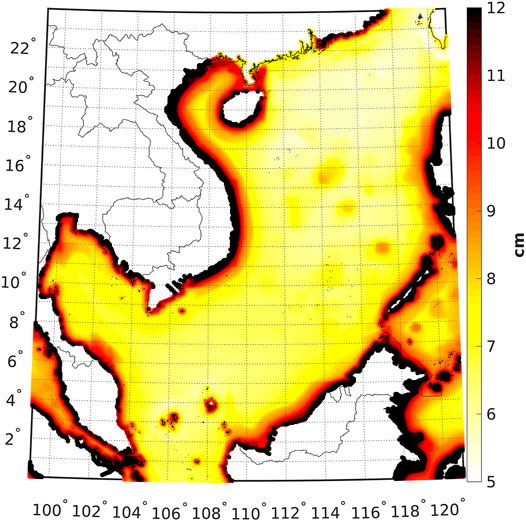
FIGURE A1. Associated errors of EGM2008 in terms of quasi-geoid heights.
Keywords: global geopotential model, model assessment, heterogeneous gravity data, ocean reanalysis data, mean dynamic topography, geostrophic velocities
Citation: Wu Y, He X, Luo Z and Shi H (2021) An Assessment of Recently Released High-Degree Global Geopotential Models Based on Heterogeneous Geodetic and Ocean Data. Front. Earth Sci. 9:749611. doi: 10.3389/feart.2021.749611
Received: 29 July 2021; Accepted: 31 August 2021;
Published: 14 September 2021.
Edited by:
Jinyun Guo, Shandong University of Science and Technology, ChinaReviewed by:
Polina Lemenkova, Institute of Physics of the Earth (RAS), RussiaCopyright © 2021 Wu, He, Luo and Shi. This is an open-access article distributed under the terms of the Creative Commons Attribution License (CC BY). The use, distribution or reproduction in other forums is permitted, provided the original author(s) and the copyright owner(s) are credited and that the original publication in this journal is cited, in accordance with accepted academic practice. No use, distribution or reproduction is permitted which does not comply with these terms.
*Correspondence: Yihao Wu, eWloYW93dUBoaHUuZWR1LmNu
Disclaimer: All claims expressed in this article are solely those of the authors and do not necessarily represent those of their affiliated organizations, or those of the publisher, the editors and the reviewers. Any product that may be evaluated in this article or claim that may be made by its manufacturer is not guaranteed or endorsed by the publisher.
Research integrity at Frontiers
Learn more about the work of our research integrity team to safeguard the quality of each article we publish.