 Chuyin Tian
 Guohe Huang
 Yanli Liu3
 Ruixin Duan
- 1Faculty of Engineering and Applied Science, University of Regina, Regina, SK, Canada
- 2State Key Joint Laboratory of Environmental Simulation and Pollution Control, China-Canada Center for Energy, Environment and Ecology Research, School of Environment, UR-BNU, Beijing Normal University, Beijing, China
- 3State Key Laboratory of Hydrology—Water Resources and Hydraulic Engineering, Nanjing Hydraulic Research Institute, Nanjing, China
- 4China Institute of Water Resources and Hydropower Research, Beijing, China
Evident climate change has been observed and projected in observation records and General Circulation Models (GCMs), respectively. This change is expected to reshape current seasonal variability; the degree varies between regions. High-resolution climate projections are thereby necessary to support further regional impact assessment. In this study, a gated recurrent unit-based recurrent neural network statistical downscaling model is developed to project future temperature change (both daily maximum temperature and minimum temperature) over Metro Vancouver, Canada. Three indexes (i.e., coefficient of determinant, root mean square error, and correlation coefficient) are estimated for model validation, indicating the developed model’s competitive ability to simulate the regional climatology of Metro Vancouver. Monthly comparisons between simulation and observation also highlight the effectiveness of the proposed downscaling method. The projected results (under one model set-up, WRF-MPI-ESM-LR, RCP 8.5) show that both maximum and minimum temperature will consistently increase between 2,035 and 2,100 over the 12 selected meteorological stations. By the end of this century, the daily maximum temperature and minimum temperature are expected to increase by an average of 2.91°C and 2.98°C. Nevertheless, with trivial increases in summer and significant rises in winter and spring, the seasonal variability will be reduced substantially, which indicates less energy requirement over Metro Vancouver. This is quite favorable for Metro Vancouver to switch from fossil fuel-based energy sources to renewable and clean forms of energy. Further, the cold extremes’ frequency of minimum temperature will be reduced as expected; however, despite evident warming trend, the hot extremes of maximum temperature will become less frequent.
Introduction
Distinct impacts of climate change on Canada are being observed. The increasing rate of temperature over Canada is near twice the global rate (Canada in a Changing Climate, 2019). The relevant mitigation and adaptation measures are thereby required to be updated. The first step is to generate suitable climate projections over selected study regions. Global climate models (GCMs) have been widely used to conduct large-scale climate change impact assessment through their coarse-scale climate projections (100–300 km resolution) (Wang et al., 2015; Tian et al., 2020). However, it is also necessary to evaluate the impacts of climate change at regional levels to understand their interrelationships with larger-scale socioeconomic processes and geographical features (Pérez et al., 2014; Jury et al., 2015; Notaro et al., 2015). To advance the representation of local climate, downscaling techniques are critical for obtaining high-resolution climate projections via handling the spatial mismatch between GCMs and regional climatology (Hessami et al., 2008; Roberts et al., 2019; Shrestha and Wang, 2020).
Previous studies have been conducted to develop a wide range of downscaling algorithms which can be divided into two categories: dynamic and statistical downscaling (Hewitson and Crane, 1996; Yu et al., 2020). Regional Climate Models (RCMs), the representative dynamic downscaling approach, could downscale the climate data from GCMs or continental reanalysis data through physical mechanisms. More importantly, dynamic downscaling can generate out-of-sample data that previously were not observed for climate projections (Feser et al., 2011). However, it would become difficult to obtain high-resolution climate data through RCMs with limited time or computation resources. By contrast, by building the statistical relationship between coarse-scale atmospheric variables and locally observed climate data, statistical downscaling could quickly generate a great number of possible outcomes under moderate computation requirements (Wilby et al., 2004; Li et al., 2020).
Diverse studies aimed at using statistical downscaling algorithms to support climate change impact assessments. Wang et al. (2013) developed a statistical downscaling software, SCADS, for downscaling climate projection based on stepwise cluster analysis. An application of this software was presented to generate 10 km-resolution daily temperature and monthly precipitation projections in Toronto, ON, Canada. Bechler et al. (2015) proposed a spatial hybrid downscaling (SHD) algorithm to overcome the defect that statistical downscaling cannot well capture the extreme behavior and features of spatial structures. To further display the superiority of the proposed method, the authors applied it to the French Mediterranean basin where extreme events occurred frequently. In addition, Chen et al. (2012) provided a thorough evaluation of different downscaling methods and hydrological models with two reanalysis data, suggesting that some widely used evaluation criteria were not effective to evaluate certain downscaling approaches. GIS-based statistical downscaling methods were also common tools for handling the GCM’s poor simulation of local climatology. Ashiq et al. (2010) utilized various interpolation models within the GIS environment to downscale PRECIS precipitation data, which filled the gap in the lack of credible precipitation data for Pakistan. In detail, inverse distance weighted, local polynomial interpolation, and radial basis functions were combined as deterministic methods. The core of selected geostatistical models was ordinary kriging and its extension which relies on the spatial autocorrelation in models. Moreover, multidimensional GCM ensembles were downscaled statistically with a GIS-based downscaling environment by Gharbia et al. (2016a). Temperature, rainfall, wind speed, solar radiation, and relative humidity were projected at a finer spatial resolution applying the proposed method. Gharbia et al. (2016b) also provided the performance assessment for multi-GCM ensemble based on statistically downscaled fine-scale data through the GIS platform. Compared to a single GCM, GCMs ensemble in downscaling climate variables could effectively reflect the uncertainty, and consequently provide more reliable climate projections for further impact assessment studies.
Deep learning techniques, especially, recurrent neural network (RNN), have been widely used in modeling sequence dependencies that exist in many fields (e.g., image processing, and language translate) (Le et al., 2020; Westermann et al., 2020). Nevertheless, few applications could be found in climate downscaling field. Moreover, since vanishing/exploding gradient problems are inevitable in naïve RNN, gated recurrent unit (GRU) technique is also applied in this study. On the other hand, owing to complex microclimate system of Metro Vancouver (MV), limited studies can be found regarding its high-resolution regional climate projections.
Thus, this study will focus on MV, where thirteen of British Columbia’s thirty most populous municipalities are located. This area is experiencing evident climate change with increasing daytime and nighttime temperatures, particularly in winter, following by consequential fewer winter days with ice or frost. In addition, motivated by the success of RNN in capturing complex non-linear relationships between time-dependent data (LeCun et al., 2015), a GRU-based RNN statistical downscaling method followed by Tian et al. will be developed to generate temperature projections (both daily maximum temperature and minimum temperature) for further impact assessment of MV. Details of the case study area and developed downscaling method are given in the next section.
Overview of the Study System
MV is bordered by fold mountain ridges to the north, the Pacific Ocean to the west, and the semi-arid Fraser Valley to the east, which results in a complicated microclimate system with growing urban heat island effects (Hay and Oke, 1976; Oke, 1976). As one of the most developed regions in the province of British Columbia (BC), Canada, MV is committed to becoming a carbon-neutral region by 2050 (Arcand et al., 2018). Switching from fossil fuel-based energy sources to renewable and clean forms of energy is consequently essential to decarbonize MV’s energy system (Zeng et al., 2011). Nevertheless, evident global warming has been changing the weather patterns. For example, it may increase the summer hot days of MV. Measures such as redesign of provincial energy infrastructures are needed for mitigation and adaptation under climate change (Metro Vancouver, 2018). Therefore, it is desired that high-resolution climate projections representing local climate features of MV be generated to support further impact assessment under climate change.
To undertake high-resolution climate projections, 12 high-quality meteorological stations are selected, as shown in Figure 1. Daily minimum and maximum temperature observations at these stations are obtained from Environment and Climate Change Canada, representing the realistic climate of MV (Historical data). Temperature simulation from RCMs displays poor performances compared to these observations (Table 1). Thus, to combine the advantages of dynamical and statistical downscaling, in this study, RCM outputs (25 km × 25 km), both historical and projected, are selected to support the developed downscaling work. The outputs (WRF-MPI-ESM-LR) are acquired from the NA-CORDEX where climate projections cover most of North America (Mearns et al., 2017). NA-CORDEX is the North American component of the international CORDEX (Coordinated Regional Downscaling Experiment) program which has been providing global coordination of regional climate downscaling for improved regional climate change adaptation and impact assessment. The selected historical RCM simulations are driven by the ERA-Interim historical reanalysis; future projections are driven by a GCM (MPI-ESM-LR) using representative concentration pathways 8.5 (RCP 8.5). With the local-scale observations over MV, the GRU-based RNN statistical downscaling model (detailed information is displayed in the next section) will be developed to correct/downscale gridded simulations (daily maximum/minimum temperature) from the selected RCM. The time series is divided into two time slots, i.e., 1986–1995 for calibration, and 1996–2005 for validation.
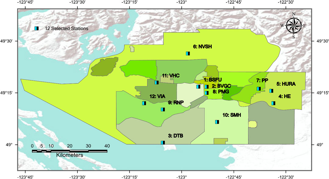
FIGURE 1. The spatial distribution of 12 selected meteorological stations.
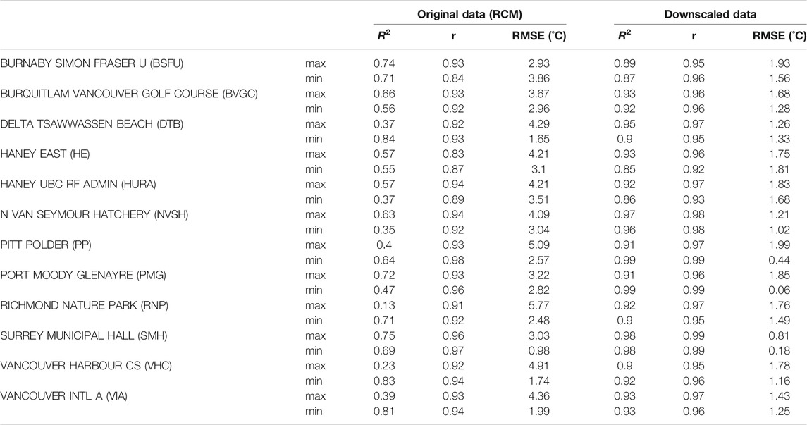
TABLE 1. Original performance of RCM outputs and validation results (all monthly data between 1996 and 2005) of the developed downscaling model.
Gated Recurrent Unit-Based Recurrent Neural Network Downscaling Model
Deep learning with multiple hidden layers is employed to represent complex functions in a series of fields (e.g., image analysis, language analysis, and runoff prediction) (Ordieres-Meré et al., 2020). Recurrent neural network (RNN, first developed by Hopfield (2018)), as a class of deep learning, has been applied to capture complex non-linear relationships, especially for time-dependent data as it allows forward and backward connections among time steps. It is found that with acceptable correlation, RNN performs better ability to capture the non-linear relationship than some traditional data-driven models. Considering the complicated non-linear relationship that exists between relatively coarse-scale simulation and realistic temperature observations, RNN statistical downscaling model followed by Tian et al. (2021) is developed for generating high-resolution temperature projections for MV. The minimum and maximum temperature projections from RCM will be downscaled, respectively.
RNN basically consists of the input layer, multiple hidden layers, and the output layer, as expressed in Eq. 1. Since the superiority of back propagation arithmetic (Li et al., 2010), RNN models can display impressive memory ability to store information from the last time step, and then decide the current outputs combined with the current outputs. However, when the time steps are large, the deeper layer is, the easier would the error of partial derivative accumulate. Specifically, the gradient will get quite small, leading to the weight in larger time steps becoming constant, which is generally known as the vanishing gradient problem. By contrast, substantial updates of weights in antecedent time steps, i.e., exploding gradient, will also significantly impact the accuracy of RNN training.
where angle brackets denote an activation function; xi is the input variable; Wi is the vector of weight assigned to corresponding input variable; b is the bias term.
Gated recurrent unit (GRU) technique is developed to handle the above-mentioned vanishing/exploding gradient problem. Different from a typical RNN, a reset gate and update gate are added in the hidden block (as shown in Figure 2), which aimed to forget the unnecessary state/input from the last/current time step. Thus, it can effectively avoid the vanishing/exploding gradient problem, and meanwhile, make the computation simpler. Albeit the application of GRU-based RNN in statistical downscaling is still in infancy, it has been demonstrated to perform better capability to capture time-dependent relationships with limited correlation between simulation and observation (LeCun et al., 2015). In detail, the GRU-based RNN can be represented as follows:
where W and U are related weights; Ugu is the update gate aimed to learn long-term dependency relationship between coarse-scale RCM simulation and temperature observation, which is determined by both hidden state from the last time step
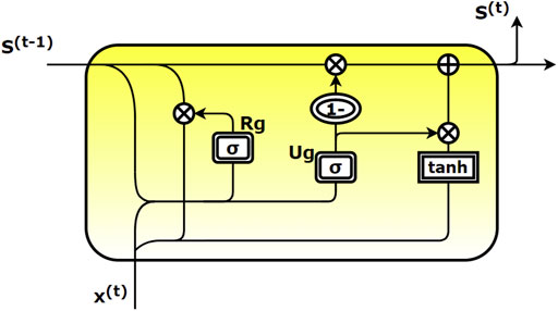
FIGURE 2. Neuron network of GRU.
In addition, to avoid over-fitting, dropout technique is applied in this study. Specifically, certain probabilities will be assigned in k neurons of a certain layer; in this way, relevant parameters will not be updated within each training iteration. That is, the final cell state would not be overly reliant on certain neurons of the hidden layer. The detailed structure and model settings can refer to Tian et al. (2021). Besides, three model evaluation criteria, i.e., determinant coefficient (R2), root mean square error (RMSE), and correlation coefficient (r), are used to evaluate the GRU-based RNN statistical downscaling.
Results and Discussion
Validation Results
To validate the calibrated GRU-based RNN downscaling model, the daily maximum and minimum temperatures in the baseline period (i.e., 1985–2005) are generated via the proposed downscaling model. The produced temperature values are then compared with meteorological observations at 12 selected stations of MV. The R2, RMSE, and r are calculated as indexes to characterize the downscaling capability of the developed approach. The validation results of monthly maximum and minimum temperature for observation and simulated values at the 12 weather stations are displayed in Table 1. Also, temperature observations are compared to the original outputs from RCM, indicating the necessity of downscaling work.
It is quite clear that for maximum temperature, most of the R-squared coefficients over the 12 meteorological stations are higher than 0.88. The highest value could be achieved at 0.98 (SMH station), while the lowest value is obtained at BSFU station (0.89). The overall performance of the presented downscaling model for maximum temperature is stabilized with the average R-square value being 0.93. Compared to the outputs of RCM, the other two indexes (r and RMSE) also suggest the good downscaling capability of the developed model. For instance, the value of RMSE at VHC station could be decreased from 4.91–
To further investigate the performance of the presented downscaling model, the monthly means of maximum and minimum temperature are compared between the simulated outputs and the observed temperature data. As displayed in Figures 3, 4, apart from few stations (e.g., HE and PMG stations) showing evident under- or overestimate compared to observations, most of the simulated temperature could well fit with the monthly variation of observations, especially for the stations with high R2/RMSE values (e.g., PP and SMH stations). In other words, the proposed downscaling model is able to well capture the overall seasonal and spatial patterns of MV. This further affirms its acceptable performance in simulating both maximum and minimum temperature at 12 selected weather stations. In addition, to filter out potential effect of annual cycle on the performance of the developed downscaling model, seasonal (i.e., spring, summer, autumn, and summer) validation is undertaken to further indicate the model’s effectiveness (see Supplementary Tables S1–S4). Despite with relatively poor performance in winter owing to quite limited correlation between RCM simulations and observations, significant improvement could be found for most of the stations compared to validation results of original RCM outputs, which suggests that the developed downscaling model is able to correct RCM seasonal errors. Therefore, albeit complex microclimate resulting in limited researches regarding the downscaling work at MV, the developed GRU-based RNN downscaling model is demonstrated to be effective to downscale the daily maximum and minimum temperature of MV.
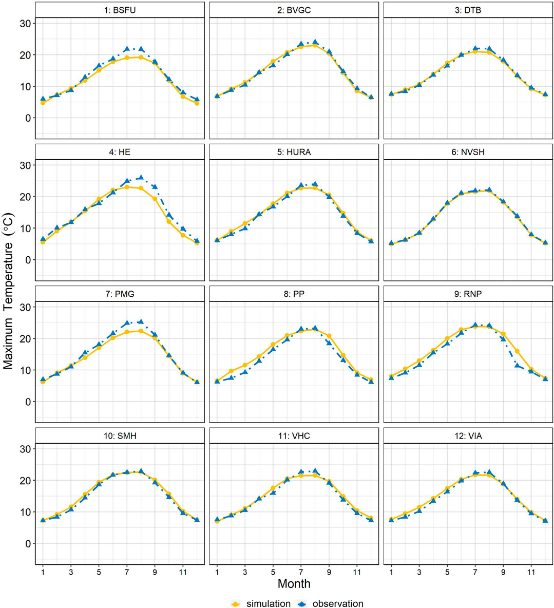
FIGURE 3. Monthly comparisons between maximum temperature simulation and observation.
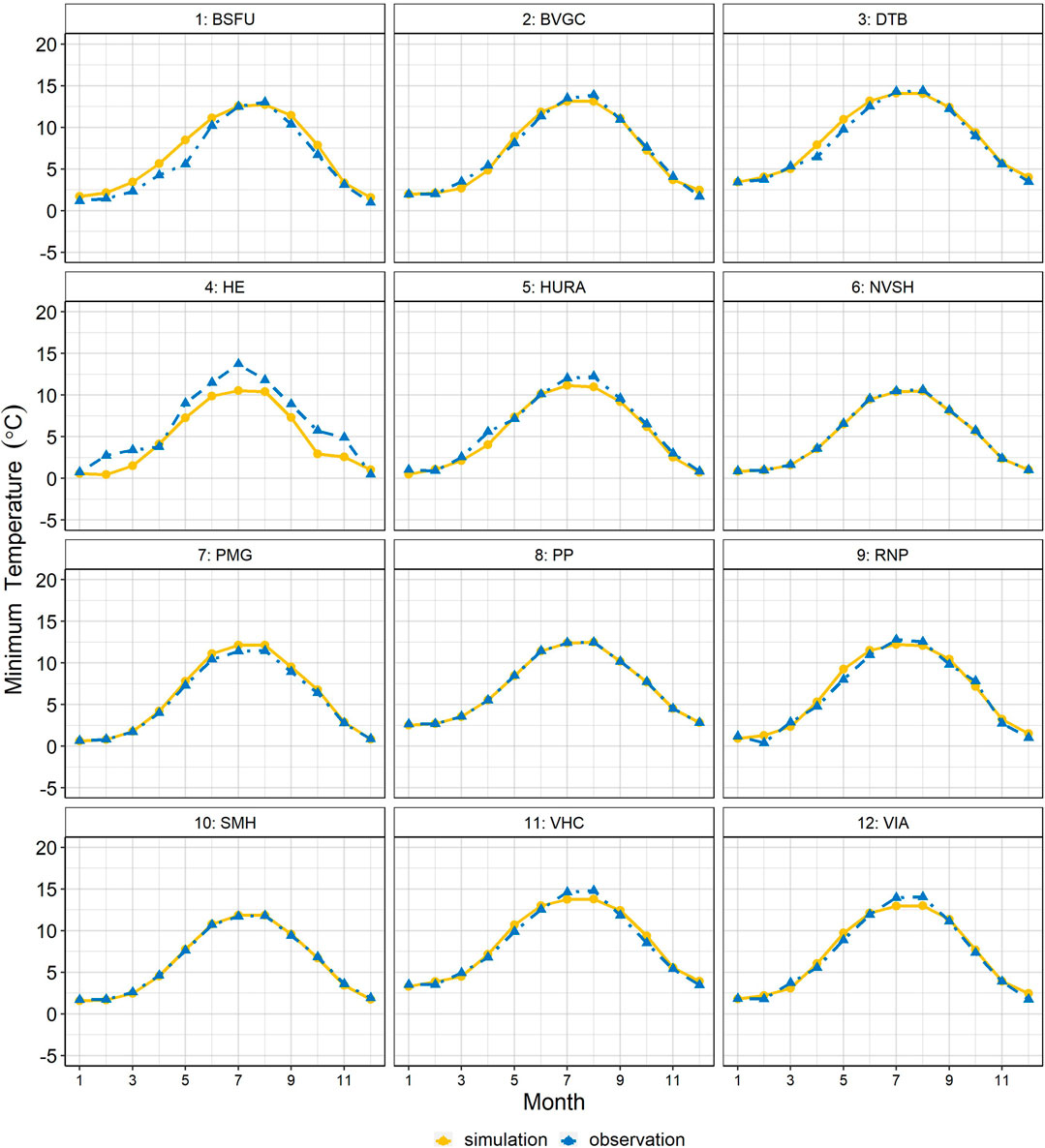
FIGURE 4. Monthly comparisons between minimum temperature simulation and observation.
Projections of Future Daily Temperature
High-resolution temperature projections for MV are obtained from 2035 to 2100 by downscaling the 25 km outputs from WRF under RCP 8.5 scenarios with the validated GRU-based RNN downscaling model. The trend analysis in daily maximum and minimum temperature is then applied to understand future changing tendency across the selected 12 stations of MV under RCP 8.5 scenario. It should be noted that p-value < 0.01 (α = 0.01) suggests that the future temperature performs a statistically significant tendency during 2035–2100. Figure 5 displays the downscaled projections of daily maximum temperature, and future tendencies of 12 weather stations which are estimated by Sen’s slope estimator (Dong et al., 2021; Song et al., 2021). It can be seen that all stations show consistent and remarkable warming trends with all of the probability values being less than 0.0001. The trend at each station also tells a different story owing to the spatial pattern of MV. The most significant increasing trend is projected to warm by approximately 0.0037°C per month for NVSH station, which means that NVSH station would increase ∼2.9°C by 2100. Also, the coastal station (e.g., DTB station) shows a similar warming trend (0.0036°C per month), taking second place among 12 meteorological stations. One may be easy to ignore is that both coastal (DTB and SMH stations) and inland stations (NVSH and PP stations) display significant warming trends in the next 65 years, which further highlights the complex climate context of MV. By contrast, the estimated warming trends at stations in highly urbanized regions such as VIA station (City of Richmond, 0.0025°C per month) and VHC station (City of Vancouver, 0.0019°C per month) are not the most significant as expected. In addition, the lowest warming tendency is estimated at BSFU station located in City of Burnaby. Compared to varying warming trends for maximum temperature, the degree of daily minimum temperature increasing is more consistent as shown in Figure 6. Similarly, the hypothesis testing indicates that 12 meteorological stations will have significant changes in the next 65 years. Instead of displaying relatively different warming trends for the maximum temperature, the trends of minimum temperature ranges at a comparatively lower level (from 0.0022°C to 0.0031°C per month). City of Richmond and City of Vancouver remains at the middle level of the warming trend, with the same trend value of 0.0024°C per month. On the other hand, a much more significant warming trend (0.0026°C per month) is displayed in the minimum temperature over BSFU station, in comparison with its maximum temperature. Furthermore, similar to the pattern of maximum temperature, both coastal and inland stations (DTB and NVSH) display consistently noticeable warming tendency; the minimum temperature would increase by 2.34°C to the end of this century. Despite less variability of trend values, the average value for monthly minimum temperature could still be as high as 0.0027°C per month for the whole MV region.
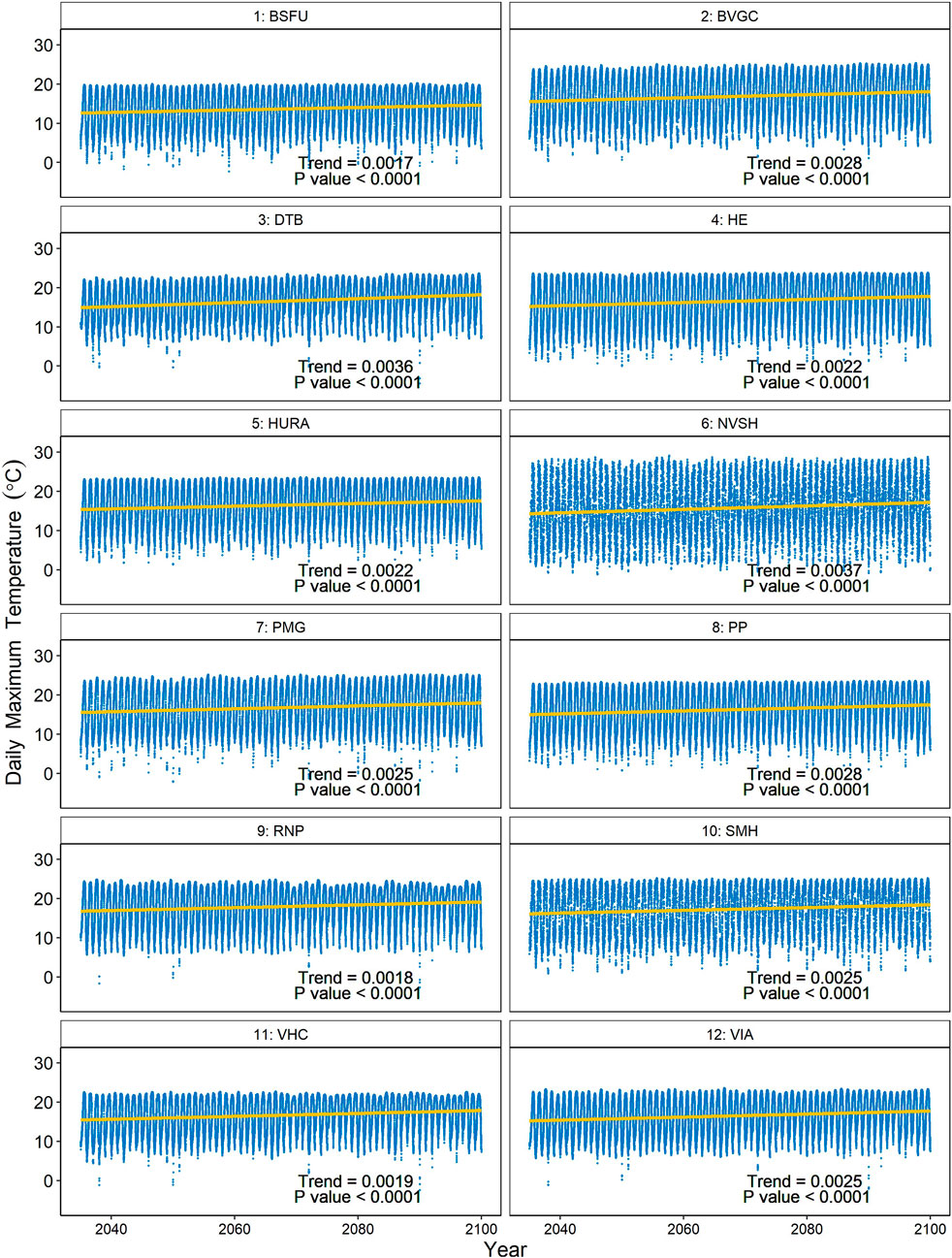
FIGURE 5. Projected trends of daily maximum temperature between 2035 and 2100.
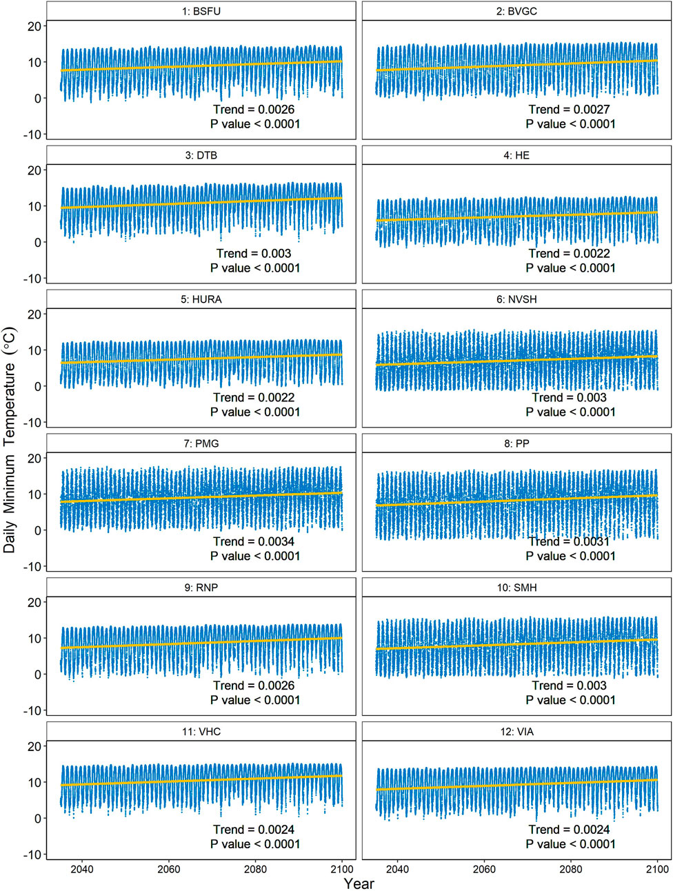
FIGURE 6. Projected trends of daily minimum temperature between 2035 and 2100.
Further, Figures 7, 8 present projected time series of maximum and minimum temperature at annual and seasonal time scales over the 12 weather stations from 2035 to 2100. For both plots, it is quite clear that all 4 seasonal time series display increasing temporal patterns from 2035 to the end of this century, which further confirms mentioned trend analysis. Interestingly, the increasing tendency in summer is not quite significant as expected, especially for maximum temperature. This suggests that even under RCP 8.5 scenario, the frequency of extreme hot events would not increase substantially, which seems good news for MV. On the other hand, it can be seen that winter and spring time scales have more predominant temporal variability. Considering these two patterns, MV is projected to experience less seasonal temperature variability under the global warming trend. Besides, maximum temperature values fluctuate between 2035 and 2060 with a relatively significant peak between 2060 and 2080, and continuously undulate with an overall increasing tendency instead of a constantly rising trend. Specifically, the patterns of HURA and VIA stations are relatively notable. Moreover, consistent plunges across 12 stations could be found in the wintertime series around 2065. By contrast, projected mean values on annual and autumn’s time scales display successive warming trends with little temporal variability. Accordant with the results of trend analysis, the maximum temperatures of NVSH and DTB stations increase consistently with constant notable crawling. As for the minimum temperature plot (Figure 8), it displays similar overall patterns with that for maximum temperature. The difference is, more evident fluctuations between 2035 and 2060 are shown in winter and spring. Besides, there are sharper increases between 2060 and 2070 compared to that of maximum temperature. The annual warming tendency is not as pronounced as that for maximum temperature but more consistent, which further demonstrates the comparison in previous trend indexes.
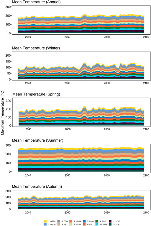
FIGURE 7. Annual and seasonal time series of projected daily maximum temperature between 2035 and 2100.
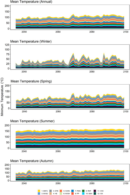
FIGURE 8. Annual and seasonal time series of projected daily minimum temperature between 2035 and 2100.
To better explore future changes of projected temperature in the 12 meteorological stations, the future projections of daily maximum and minimum temperature are divided into three periods (the 2030s, 2050s, and 2080s, i.e., 2035–2054, 2055–2074, and 2075–2100). The projected climate changes are calculated based on the mean temperature of three periods under RCP 8.5 as well as that of the 20 years baseline, i.e., historical periods from 1985 to 2005. The projections of changes in daily maximum and minimum temperature under RCP 8.5 scenario could be further analyzed at the 12 selected weather stations.
Figure 9 depicts the baseline simulated maximum and minimum temperature, as well as future annual temperature changes of 12 selected stations for the 2030, 2050, and 2080 s under RCP 8.5. RNP and SMH stations (located at City of Richmond and City of Surrey, respectively) show the highest maximum temperature during the baseline period; while for the minimum temperature, VHC and DTB (located at City of Vancouver and District of Delta, respectively) are the top two stations. As for the future changes, the results suggest that the simulated annual maximum temperature changes would increase consistently across the 12 weather stations from the near term to the end of this century. Instead of RNP and SMH stations, the changes in the annual maximum temperature for District of Delta (DTB station) and City of Coquitlam (PMG station) are the most significant, with change values being 1.76°C and 1.67°C in the 2030s, 2.69°C and 2.40°C in the 2050s, as well as 3.93°C and 3.26°C to the end of this century. These cities would face more serious positive changes in maximum temperature, which may increase the cooling requirement of buildings within summer. In addition, NVSH station ranks third and also reveals conspicuous positive changes. The projected change of its maximum temperature would be 1.53°C in the near term, 2.48°C in the 2050s, and 3.44°C in the 2080s, respectively. It is interesting that even if some stations (e.g., VIA and VHC stations) display relatively gentle increasing rates in previous trend analysis, considerable positive change will still occur. In particular, to the end of this century, almost half of the selected stations will increase by ∼3°C in comparison with the baseline maximum temperature. Potential impacts from positive changes under the high radiative value of RCP 8.5 still have to be faced in the future. For the minimum temperature, similar to patterns of the maximum temperature, the entire MV region (12 stations) displays an obvious rising tendency from the 2030s–2080s. Even for the least positive change of PP station located in District of Pitt Meadows would increase from 0.29°C in the 2030s to 1.16°C in the 2050s, and then continue to as high as 2.16°C in the 2080s. The greatest warming in the minimum temperature still occurs in the PMG station (City of Coquitlam); by the 2080s, the changes could reach as high as 4.09°C relative to the historical baseline. Moreover, one of the highly urbanized cities, City of Richmond, shows quite a bit increase compared to historical climate. The positive change could reach 3.14°C at the end of this century. This may cause by the relatively lower minimum temperature in the historical baseline. Comparatively, it is interesting to note that in many stations, the rises of minimum temperature are greater than those of maximum temperature, indicating the daily temperature range of these stations is projected to become narrow under RCP 8.5 scenario.
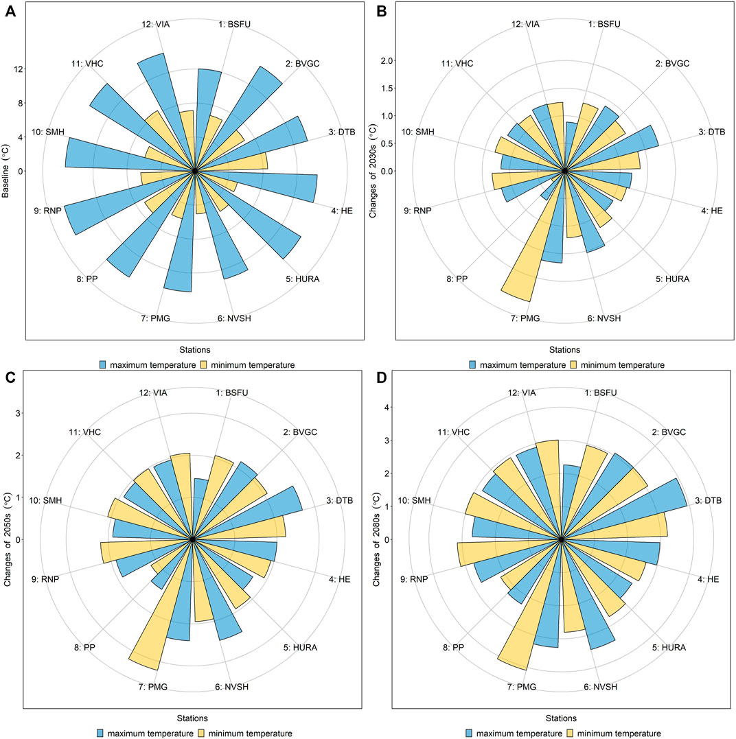
FIGURE 9. Baseline temperature (A) and projected changes over 2030s (B), 2050s (C), and 2080s (D).
Comparatively, the annual minimum temperature shows more apparent spatial variability especially in the 2030s where the highest positive change (PMG station) could achieve at more than 8 times of the least increase relative to the baseline. Albeit less spatial pattern is found for the annual minimum temperature, the rising amplitude compared to historical climate is commensurate with that for annual maximum temperature in most stations. Overall, such a continuous rising tendency may raise the temperature of MV by 2.28°C by the end of this century. Both coastal and inland cities are likely to have a pronounced climate warming trend. Unexpectedly, under RCP 8.5 scenario, i.e., scenario for long-term high energy requirement and GHG emissions without any climate adaptation policies, highly urbanized cities with developed economy will not experience more frequent hot extremes. By contrast, evident increases are displayed in the projected minimum temperature, narrowing the daily temperature difference in these stations.
To understand temperature projections’ temporal changes over MV, monthly maximum and minimum temperature changes are calculated for the specific period, i.e., from 2075 to 2095. Figure 10 displays monthly baseline maximum temperature and specific changes of 2,075–2,095 at the 12 meteorological. It is clear that positive changes are shown in almost every month; especially, all the 12 weather stations consistently have significant increases in January/February/March (the average change of all stations in these 3 months could reach as high as 2.99°C). The mere exception to this is that few changes could be found in July and August for most of the stations, which further demonstrates the concluded stable state during the summer period. The results also show that for most stations, changes of the maximum temperature in spring and winter are greater than those in autumn and summer. For instance, in City of Surrey (SMH station), the positive change values of winter and spring are 2.75°C and 3.52°C, while those for spring and summer would be only 2.03°C and 1.38°C, respectively. The highest positive change would be 6.47°C of NVSH station in March rather than 3.39°C of PMG station. Most of the increases in maximum temperature for PMG and DTB stations are contributed by winter and spring. Stations with relatively moderate warming trends such as VIA station also perform considerable increases in all months with the largest increase of 5.16°C occurring in October and an average positive change of 2.91°C. As for the monthly minimum temperature under RCP 8.5 scenario shown in Figure 11, it can be seen that compared to the increases in monthly maximum temperature, more significant rises in winter and spring are displayed in monthly minimum temperature for most of the selected stations. More specifically, the average value in winter would be 4.73°C, while that for maximum temperature in Figure 10 is only at 2.97°C. In addition, evident increases could also be found in July and August, which is consistent with previous findings. PMG stations show the most remarkable positive changes in nearly every month, causing the highest increases in the aforementioned annual mean. Overall, as shown in these two figures, it is quite clear that under RCP 8.5 scenario, the monthly variability will be substantially reduced across all the weather stations. The difference between the maximum and minimum temperature will also be narrowed to the end of this century. The results are consistent with previous conclusions.
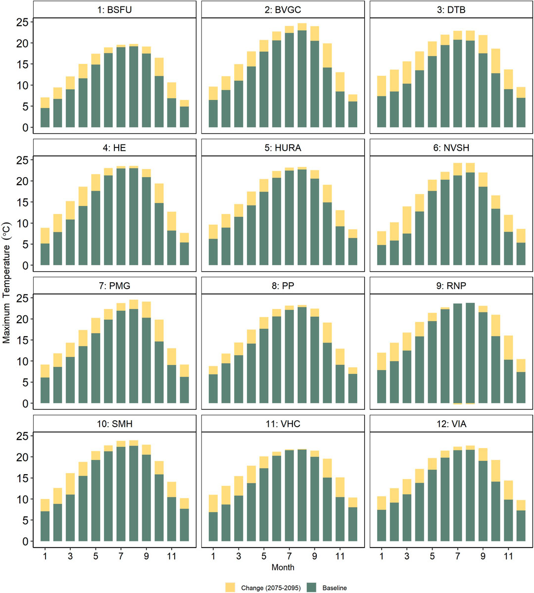
FIGURE 10. Monthly baseline and projected changes of 2075–2095 for maximum temperature.
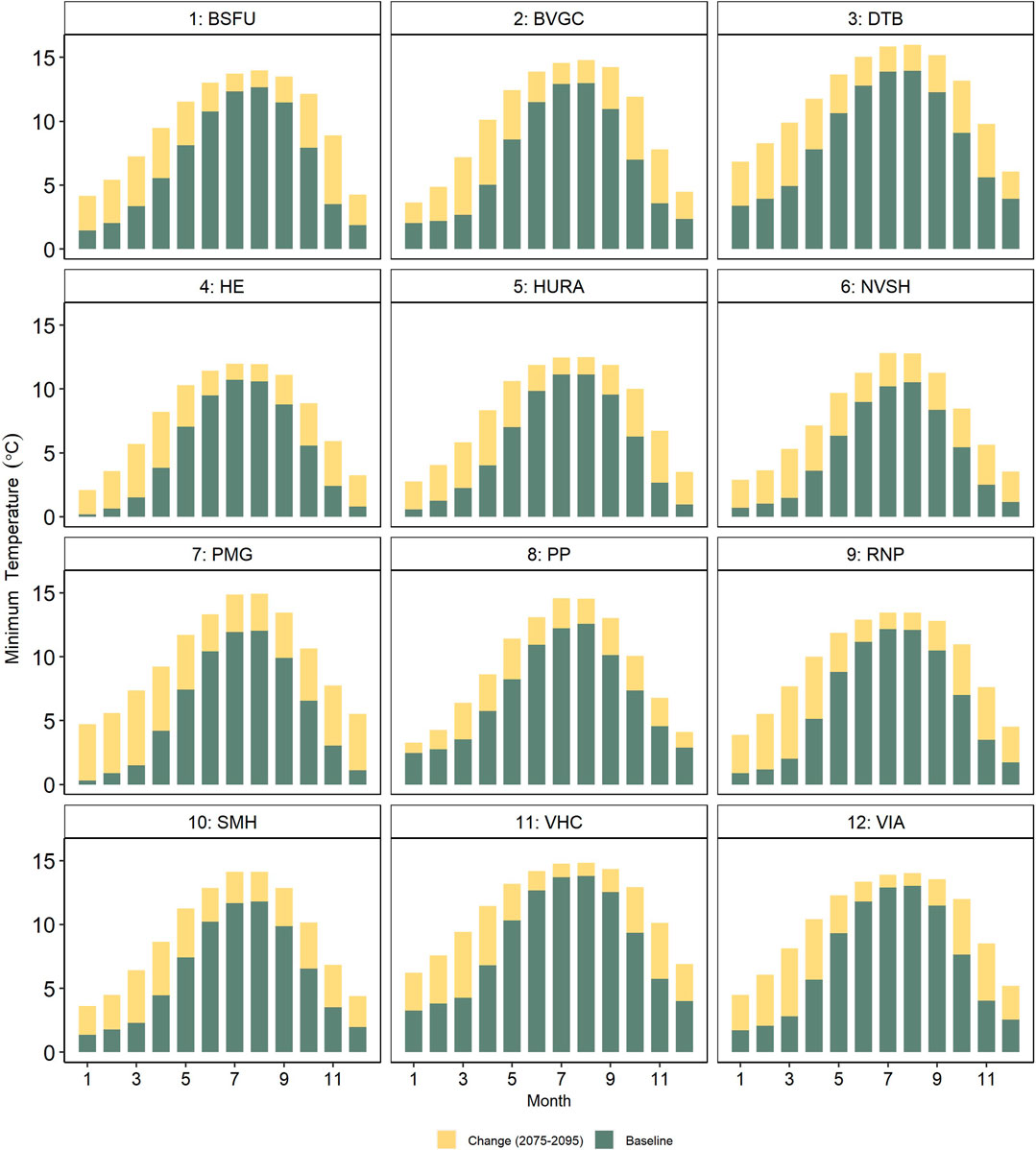
FIGURE 11. Monthly baseline and projected changes of 2075–2095 for minimum temperature.
Figure 12 displays the ∼20 years distributions (baseline period and 2075–2095, respectively) of 12 meteorological stations. Despite the annual increases of extreme maximum temperature are not significant at most of the stations as mentioned before, the frequency of relatively lower temperature is reduced evidently since “violin” distributions of all the stations get to top-heavy. Moreover, as shown in this figure, the hot extreme’s frequency would not increase substantially, which is consistent with the above-mentioned analysis. Furthermore, since NVSH station shows the most significant warming trend from 2035 to 2100, the frequency of higher and lower temperatures seems to interchange in 2075–2095, compared to the baseline period, which is different from other stations. For daily minimum temperature, there are four stations (i.e., NVSH, PMG, PP, and SMH stations) displaying similar patterns, which further highlights more notable rises in comparison with maximum temperature. In addition, top-heavy “violin” distributions are more common in Figure 12B; the frequency of cold extreme will experience massive declines.
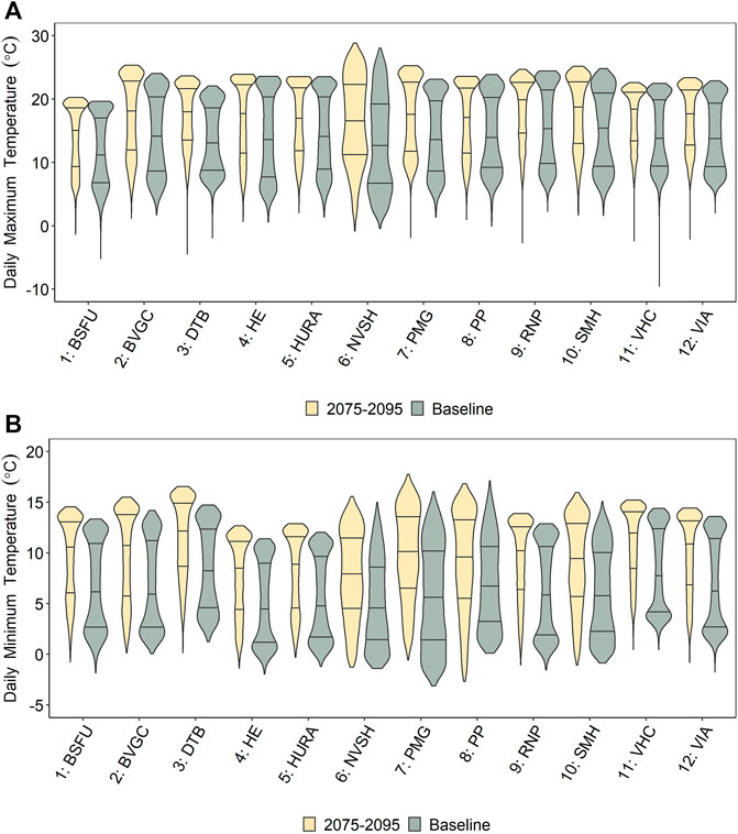
FIGURE 12. Frequency distributions of daily maximum (A) and minimum (B) temperature between 2075 and 2095.
Conclusion
In this study, a GRU-based RNN downscaling approach was developed to tackle the spatial mismatch between coarse-scale climate simulation and regional climatology for improving the representation of local future climate across MV. The complex microclimate systems under the context of the alpine and coastal areas are usually difficult to be simulated by GCMs and even RCMs. The proposed downscaling model was demonstrated (by three indexes, namely, R2, RMSE, and r) to perform competitive ability to capture the regional climatology of MV. The effectiveness was further highlighted by the monthly comparison, indicating that the GRU-based RNN downscaling model could well simulate the MV’s overall seasonal and spatial patterns.
The presented downscaling approach was then applied to generate regional high-resolution climate projections of the maximum and minimum temperature from 2,035 to 2,100 under RCP 8.5. Trend analysis in the next 65 years was first conducted by Sen’s slope algorithm, which disclosed that both maximum and minimum temperature would consistently increase over the 12 selected weather stations. Both coastal and inland regions may experience more significant successive warming in the future, which revealing the complex microclimate of MV. These results were accordant with annual and seasonal analysis for temporal patterns. Furthermore, the future temperature changes were analyzed to better understand the potential impacts of climate change on MV under a high RCP scenario. It was indicated that the entire MV (12 stations) displayed obvious gradually increasing positive changes from the 2030s–2080s relative to the baseline climate of each station. In addition, both annual maximum and minimum temperature shows apparent spatial variability, especially by the 2080s. More importantly, it can be also found that with negligible increases in summer (e.g., RNP and VHC stations) and notable rises in winter and spring, the seasonal temperature variability would be reduced substantially. Further, surprisingly, despite evident warming trends, the hot extremes of maximum temperature will become less frequent. On the other hand, the cold extreme’s frequency of minimum temperature will be reduced as expected.
Overall, the presented GRU-based RNN downscaling approach could effectively capture the statistical relationship between RCM outputs and realistic climatology, and consequently combine advantages of both dynamic and statistical methods. Thus, maximum and minimum temperature projections could provide effective support for further regional impact assessment in MV. However, notwithstanding it can reflect local climate features based on dynamical downscaling (RCM outputs), the systematic errors in the simulated fields hidden within RCMs would be transferred into the statistical downscaling process, which may cause relatively poor performance of some station’s validation (especially in winter) in this study. Besides, a wide range of factors (e.g., input data, model selection, and parameter setup) may result in multiple uncertainties, which would impact the robustness of a single GCM/RCM model. Future research is thereby desirable to introduce multiple GCM/RCM ensembles and further investigate the inherent uncertainties to advance the performance of the proposed downscaling approach.
Data Availability Statement
The raw data supporting the conclusion of this article will be made available by the authors, without undue reservation.
Author Contributions
CT: Conceptualization, Methodology, Software, Data curation, Formal analysis, Writing—original draft. GH: Supervision, Project administration, Funding acquisition, Resources. YL: Guidance, Writing—review and editing. DY: Guidance, Writing—review and editing. FW: Software, Writing—review. RD: Software, Writing—review.
Funding
This research was supported by the National Key Research and Development Plan (2016YFA0601502), Canada Research Chair Program, Natural Science and Engineering Research Council of Canada, Western Economic Diversification (15269), and MITACS.
Conflict of Interest
The authors declare that the research was conducted in the absence of any commercial or financial relationships that could be construed as a potential conflict of interest.
Publisher’s Note
All claims expressed in this article are solely those of the authors and do not necessarily represent those of their affiliated organizations, or those of the publisher, the editors and the reviewers. Any product that may be evaluated in this article, or claim that may be made by its manufacturer, is not guaranteed or endorsed by the publisher.
Supplementary Material
The Supplementary Material for this article can be found online at: https://www.frontiersin.org/articles/10.3389/feart.2021.742840/full#supplementary-material
References
Arcand, A., Wiebe, R., McIntyre, J., and Bougas, C. (2018). “Metropolitan Outlook 1: Economic Insights into 13 Canadian Metropolitan Economies,” in Ottawa: Conference Board of Canada. Available at: https://www.conferenceboard.ca/e-library/abstract.aspx?did=9923.
Ashiq, M. W., Zhao, C., Ni, J., and Akhtar, M. (2010). GIS-based High-Resolution Spatial Interpolation of Precipitation in Mountain-plain Areas of Upper Pakistan for Regional Climate Change Impact Studies. Theor. Appl. Climatol. 99, 239–253. doi:10.1007/s00704-009-0140-y
Bechler, A., Vrac, M., and Bel, L. (2015). A Spatial Hybrid Approach for Downscaling of Extreme Precipitation fields. J. Geophys. Res. Atmos. 120, 4534–4550. doi:10.1002/2014JD022558
Bush, E., and Lemmen, D. S. (Editors) (2019). Canada’s Changing Climate Report. Ottawa, ON: Government of Canada, 444. Available at: https://www.nrcan.gc.ca/sites/www.nrcan.gc.ca/files/energy/Climate-change/pdf/CCCR_FULLREPORT-EN-FINAL.pdf
Chen, H., Xu, C.-Y., and Guo, S. (2012). Comparison and Evaluation of Multiple GCMs, Statistical Downscaling and Hydrological Models in the Study of Climate Change Impacts on Runoff. J. Hydrol. 434-435, 36–45. doi:10.1016/j.jhydrol.2012.02.040
Dong, C., Huang, G., and Cheng, G. (2021). Offshore Wind Can Power Canada. Energy 236, 121422. doi:10.1016/j.energy.2021.121422
Feser, F., Rockel, B., von Storch, H., Winterfeldt, J., and Zahn, M. (2011). Regional Climate Models Add Value to Global Model Data: a Review and Selected Examples. Bull. Am. Meteorol. Soc. 92, 1181–1192. doi:10.1175/2011bams3061.1
Gharbia, S. S., Gill, L., Johnston, P., and Pilla, F. (2016a). Multi-GCM Ensembles Performance for Climate Projection on a GIS Platform. Model. Earth Syst. Environ. 2, 1–21. doi:10.1007/s40808-016-0154-2
Gharbia, S. S., Johnston, P., Gill, L., and Pilla, F. (2016b). Using GIS Based Algorithms for GCMs' Performance Evaluation. Proc. 18th Mediterr. Electrotech. Conf. Intell. Effic. Technol. Serv. Citizen, MELECON 2016, 1–6. doi:10.1109/MELCON.2016.7495476
Hessami, M., Gachon, P., Ouarda, T. B. M. J., and St-Hilaire, A. (2008). Automated Regression-Based Statistical Downscaling Tool. Environ. Model. Softw. 23, 813–834. doi:10.1016/j.envsoft.2007.10.004
Hewitson, B., and Crane, R. (1996). Climate Downscaling: Techniques and Application. Clim. Res. 7, 85–95. doi:10.3354/cr007085
Hopfield, J. J. (2018). Neural Networks and Physical Systems with Emergent Collective Computational Abilities. Proc. Natl. Acad. Sci. U S A. 79, 2554–2558. doi:10.1073/pnas.79.8.2554
Jury, M. W., Prein, A. F., Truhetz, H., and Gobiet, A. (2015). Evaluation of CMIP5 Models in the Context of Dynamical Downscaling over Europe. J. Clim. 28, 5575–5582. doi:10.1175/jcli-d-14-00430.1
Le, H. V., Bui, Q. T., Bui, D. T., Tran, H. H., and Hoang, N. D. (2020). A Hybrid Intelligence System Based on Relevance Vector Machines and Imperialist Competitive Optimization for Modelling Forest Fire Danger Using GIS. J. Environ. Inform. 36, 43–57. doi:10.3808/jei.201800404
LeCun, Y., Bengio, Y., and Hinton, G. (2015). Deep Learning. Nature 521, 436–444. doi:10.1038/nature14539
Li, Y. F., Li, Y. P., Huang, G. H., and Chen, X. (2010). Energy and Environmental Systems Planning under Uncertainty-An Inexact Fuzzy-Stochastic Programming Approach. Appl. Energ. 87, 3189–3211. doi:10.1016/j.apenergy.2010.02.030
Li, Z., Li, J. J., and Shi, X. P. (2020). A Two-Stage Multisite and Multivariate Weather Generator. J. Environ. Inform. 35.
Mearns, L. O., McGinnis, S., Korytina, D., Arritt, R., Biner, S., Bukovsky, M., et al. (2017). The NA-CORDEX Dataset, Version 1.0. NCAR Clim. Data Gateway. Boulder, Colorado: Boulder North Am. CORDEX Progr.
Metro Vancouver (2018). Climate 2050 Strategic Framework: Energy. Available at: http://www.metrovancouver.org/services/air-quality/AirQualityPublications/C2050-IssueAreaSummary-Energy.pdf#search=generating energy from waste.1
Notaro, M., Bennington, V., and Lofgren, B. (2015). Dynamical Downscaling-Based Projections of Great Lakes Water Levels*+. J. Clim. 28, 9721–9745. doi:10.1175/jcli-d-14-00847.1
Oke, T. R. (1976). The Distinction between Canopy and Boundary‐layer Urban Heat Islands. Atmosphere 14, 268–277. doi:10.1080/00046973.1976.9648422
Ordieres-Meré, J., Ouarzazi, J., El Johra, B., and Gong, B. (2020). Predicting Ground Level Ozone in Marrakesh by Machine-Learning Techniques. J. Environ. Inform. 36, 93–106. doi:10.3808/jei.202000437
Pérez, J. C., Díaz, J. P., González, A., Expósito, J., Rivera-López, F., and Taima, D. (2014). Evaluation of WRF Parameterizations for Dynamical Downscaling in the Canary Islands. J. Clim. 27, 5611–5631. doi:10.1175/jcli-d-13-00458.1
Roberts, J. L., Tozer, C. R., Ho, M., Kiem, A. S., Vance, T. R., Jong, L M., et al. (2019). Reconciling Unevenly Sampled Paleoclimate Proxies: a Gaussian Kernel Correlation Multiproxy Reconstruction. J. Environ. Inform. 1–10. doi:10.3808/jei.201900420
Shrestha, N. K., and Wang, J. (2020). Water Quality Management of a Cold Climate Region Watershed in Changing Climate. J. Environ. Inform. 35, 56–80. doi:10.3808/jei.201900407
Song, P., Huang, G., An, C., Xin, X., Zhang, P., Chen, X., et al. (2021). Exploring the Decentralized Treatment of Sulfamethoxazole-Contained Poultry Wastewater through Vertical-Flow Multi-Soil-Layering Systems in Rural Communities. Water Res. 188, 116480. doi:10.1016/j.watres.2020.116480
Tian, C., Huang, G., Lu, C., Zhou, X., and Duan, R. (2021). Development of Enthalpy-Based Climate Indicators for Characterizing Building Cooling and Heating Energy Demand under Climate Change. Renew. Sustain. Energ. Rev. 143, 110799. doi:10.1016/j.rser.2021.110799
Tian, C., Huang, G., and Xie, Y. (2020). Systematic Evaluation for Hydropower Exploitation Rationality in Hydro-Dominant Area: A Case Study of Sichuan Province, China. Renew. Energ.
Wang, X., Huang, G., Lin, Q., Nie, X., Cheng, G., Fan, Y., et al. (2013). A Stepwise Cluster Analysis Approach for Downscaled Climate Projection - A Canadian Case Study. Environ. Model. Softw. 49, 141–151. doi:10.1016/j.envsoft.2013.08.006
Wang, X., Huang, G., Lin, Q., Nie, X., and Liu, J. (2015). High-resolution Temperature and Precipitation Projections over Ontario, Canada: A Coupled Dynamical-Statistical Approach. Q.J.R. Meteorol. Soc. 141, 1137–1146. doi:10.1002/qj.2421
Westermann, P., Welzel, M., and Evins, R. (2020). Using a Deep Temporal Convolutional Network as a Building Energy Surrogate Model that Spans Multiple Climate Zones. Appl. Energ. 278, 115563. doi:10.1016/j.apenergy.2020.115563
Wilby, R. L., Charles, S. P., Zorita, E., Timbal, B., Whetton, P., and Mearns, L. O. (2004). Guidelines for Use of Climate Scenarios Developed from Statistical Downscaling Methods. Supporting material of the Intergovernmental Panel on Climate Change. Available from the DDC of IPCC TGCIA, 27. Available at: https://www.ipcc-data.org/guidelines/dgm_no2_v1_09_2004.pdf
Yu, B. Y., Wu, P., Sui, J., Ni, J., and Whitcombe, T. (2020). Variation of Runoff and Sediment Transport in the Huai River–A Case Study. J. Environ. Inf. 35 (2), 138–147. doi:10.3808/jei.202000429
Keywords: climate change, statistical downscaling, regional climate model, long-term projection, recurrent neural network
Citation: Tian C, Huang G, Liu Y, Yan D, Wang F and Duan R (2021) Long-Term Maximum and Minimum Temperature Projections Over Metro Vancouver, Canada. Front. Earth Sci. 9:742840. doi: 10.3389/feart.2021.742840
Received: 16 July 2021; Accepted: 14 September 2021;
Published: 27 September 2021.
Edited by:
Shan Zhao, Shandong University, ChinaReviewed by:
Ashok Kumar Jaswal, India Meteorological Department, IndiaEduardo Zorita, Helmholtz Centre for Materials and Coastal Research (HZG), Germany
Chenglong Zhang, China Agricultural University, China
Mo Li, Northeast Agricultural University, China
Copyright © 2021 Tian, Huang, Liu, Yan, Wang and Duan. This is an open-access article distributed under the terms of the Creative Commons Attribution License (CC BY). The use, distribution or reproduction in other forums is permitted, provided the original author(s) and the copyright owner(s) are credited and that the original publication in this journal is cited, in accordance with accepted academic practice. No use, distribution or reproduction is permitted which does not comply with these terms.
*Correspondence: Guohe Huang, aHVhbmdnQHVyZWdpbmEuY2E=