Landslide Scarp Assessments by Means of an Ellipse-Referenced Idealized Curved Surface

The importance of scenario investigation in landslide-related hazard mitigation planning has long been recognized, where numerical simulation with physics-based models plays a crucial role because of its quantitative information. However, a plausible failure surface is a prerequisite in conducting the numerical simulation, but it often has a high degree of uncertainty due to the complex geological structure. The present study is devoted to proposing a methodology to mimic the plausible landslide failure surface (with some uncertainty) for investigating the consequent flow paths when failure takes place. Instead of a spherical shape, an idealized curved surface (ICS) is used, where two constant curvatures are, respectively, assigned in the down-slope and cross-slope directions. A reference ellipse is introduced for constructing the associated ICS with a specified failure depth regarding these two curvatures. Through translating, rotating, or side-tilting the reference ellipse, the most appropriate ICS is figured out with respect to the assigned constraints (failure area, volume of released mass, depth of sliding interface, etc.). The feasibility and practicability of this ellipse–ICS method are examined by application to a historical landslide event and one landslide-prone area. In application to the historical event, the fitness versus the landslide scarp area and its impacts on the consequent flow paths are investigated. For the landslide-prone area, five scenarios are arranged based on the surface features and the records of gaging wells. The most plausible failure scenario is therefore suggested as the prerequisite for mimicking the consequential flow paths.

1 Introduction

Landslides, either with fast movement or in creeping motion, together with the sequential mass movement, pose severe threats to human lives as well as infrastructures in mountain areas (Dong et al., 2011; Lin et al., 2011; Iverson et al., 2015; Zhang et al., 2018; Sala et al., 2021; Van Tien et al., 2021). In the aspect of disaster mitigation/prevention plannings, the determination of the plausible failure surface is the core issue, which is closely related to the analysis of slope stability, the slide volume, and the influence area. However, the complex composition, spatial geological structure, and hydrological variations lead the determination of a precise failure surface on the natural slopes in mountain areas to a highly challenging task, especially when the field data are incomplete. Hence, the determination/prediction of a landslide failure surface and estimation of the associated volume of released mass are with a high degree of uncertainty (e.g., Jaboyedoff et al., 2019; Yeh et al., 2021).

The limit equilibrium method (LEM) and the finite element method (FEM) are the two traditional and widely employed approaches for evaluating the stability of slopes (e.g., Briaud, 2013; Shen and Abbas, 2013). The LEMs evaluate the equilibrium of a slope under the influence of gravity, where the method of slides is the most popular one. The method of slices can date back to the pioneering work of Fellenius (1927), where the soil mass is sliced into vertical elements, and the forces are analyzed on a cylindrical sliding surface to determine the factor of safety of the slope. Depending on the number of the sliced vertical elements, an equation system is derived for the conservations of force and/or moment of momentum, where additional assumptions for forces between adjacent slides are introduced as closure conditions. Hence, there are several proposals for various closure conditions, such as the ones by Bishop (1955), Janbu (1954), Janbu (1973), and Morgenstern and Price (1965) for 2D analysis and by Lam and Fredlund (1993), Huang and Tsai (2000), Huang et al. (2002), and Reid et al. (2015) explicitly for 3D stability analysis. Although the layered structure or the impacts of groundwater distribution can be included in the method of slices, a predefined sliding surface should be given as input data. This approach leads to several strategies for mimicking the sliding surface, such as the most observed circular arc, piecewise linear segments, or a combination of the both, depending on the geological condition of the investigated site, e.g., the software SLOPE/W (GEO-SLOPE International Ltd, 2012). For locating the most critical failure surface (i.e., with the lowest possible factor of safety), it turns to be a procedure of iterative search (e.g., Briaud, 2013).

The FEM is based on continuum mechanics together with appropriate constitutive laws for the stress–strain relation in analyzing the stability of slopes (Griffiths and Lane, 1999). Utilizing the FEM approach, one identifies the failure surface by the weakest zones in the calculated stress field, where significant displacement/deformation takes place. Hence, the performance of FEM highly relies on the employed constitutive models. Although the FEM methods can figure out the weakest zones, the geological conditions in mountain areas are far too complex to utilize the FEM approach with simplistic constitutive laws for a precise description of the plausible failure surface. On the other hand, one can recognize, thanks to the modern techniques of remote sensing (light detection and ranging (LiDAR), interferometric synthetic-aperture radar (InSAR), uninhabited aerial vehicle SAR (UAVSAR), or temporarily coherent point interferometry SAR (TCPInSAR), etc.), the tiny geomorphological features on the surface, such as cracks or minor scarps, for identifying and delineating the potential landslide sites (Lin et al., 2013; Stumpf et al., 2013; Delbridge et al., 2016; Lai, 2019; Wang, 2020). Along this direction, assessing the associated landslide volume and the consequential influence area is essential in disaster mitigation planning in which numerical simulation can serve as a powerful tool in scenario investigation. Thus, an efficient method for mimicking the 3D failure surface and estimating the landslide volume in various scenarios is highly requested.

For approximating the 3D failure surface, Jaboyedoff et al. (2004) and Jaboyedoff et al. (2009) proposed the Sloping Local Base Level (SLBL) method to construct a curved surface, of which the second derivative along the down-slope direction remains constant. The SLBL technique has been tested against landslides triggered by Typhoon Talas in Japan, where reasonable agreements (±35%) were achieved (Jaboyedoff et al., 2019). For studying the 3D stability of stratovolcano edifice, Reid et al. (2000) and Reid et al. (2001) suggested a spherical failure surface for analyzing the slope stability by using the LEM without considering the internal/local structures. This approach has been extended for including the spatial geological structure and groundwater patterns, as available in the software Scoops3D (see, e.g., Reid et al., 2015; Tran et al., 2018; Zhang and Wang, 2019). For a specified area (convex polygon) and a predefined volume of released mass, Kuo et al. (2020) published a method for boundary-fitted, volume-constrained, smooth minimal surface (SMS). Nearly at the same time, Tai et al. (2020) proposed the concept of an idealized curved surface (ICS) to mimic the failure surface for performing numerical simulations. The ICS consists of two constant curvatures in the down-slope and cross-slope directions, respectively, so that the ICS method can be seen as a modification of the SLBL-method or the spherical approach (Scoops3D). All these approaches (SLBL, spherical approach, SMS, or ICS) aim at a low cost but efficient estimation, where the stratigraphy and geological structures can be omitted. Hence, they are not able to provide predictions with a high degree of precision. Nevertheless, higher tolerance in prediction would be allowed in the application of scenario investigations for hazard mitigation planning because the measured field data are subject to a certain degree of uncertainty.

In the present study, we adopt the concept of an idealized curved surface (ICS) to mimic the plausible failure surface as well as to define the associated scarp area. Because of the characteristic of two constant curvatures, a reference ellipse is introduced for constructing the ICS. For an assigned area (delineated area) and its associated volume of released mass, we look for the most appropriate ICS by adjusting (translating, rotating, or tilting) the reference ellipse and by trying a range of failure depth. Because the most appropriate ICS is a smooth surface, there are certainly discrepancies between the predicted scarp area and the reference one. In contrast to the smooth minimal surface (SMS) method Kuo et al. (2020), where the boundary of the predicted failure surface fits the assigned border exactly, this approach relaxes the constrain and allows modification of the area as well as released volume for matching some specified area. Because of the high degree of uncertainty, the potential site of landslide sometimes has to be modified based on updated measurement (e.g., the records of inclinometer or groundwater level). The proposed ellipse–ICS approach provides the freedom of flexible coverage for minimizing the discrepancy.

2 Reference Ellipse and Idealized Surface for Failure Surface

2.1 Idealized Curved Surface

Based on the geomorphological concept, Tai et al. (2020) proposed an idealized curved surface (ICS) as the plausible landslide failure surface in computation for the consequent flow paths. The key feature of the ICS is that the surface is defined by two distinct curvatures remaining constant in the main (down-slope) and transverse (cross-slope) directions, respectively. As shown in Figure 1A, the ICS is fundamentally constructed by four points, p_a, p_b, p_c, and p_d, where $\overline{p_a{p}_b}$ is along the down-slope direction and $\overline{p_c{p}_d}$ lies in the transverse direction. In the work of Tai et al. (2020), p_a is assigned to lie at the upper part of the scarp area and p_b is at the lower points, while the vertical section of $\overline{p_c{p}_d}$ perpendicularly crosses the midpoint of $\overline{p_a{p}_b}$ (see Figures 1A,B). In other words, $\overline{p_a{p}_b}$ and $\overline{p_c{p}_d}$ are perpendicular to each other in the top view, but they are generally not on the sample plane (i.e., d_D ≠ d_T). Besides, $\overline{p_c{p}_d}$ is not always symmetric about $\overline{p_a{p}_b}$ (cf. Figure 1B). In the present study, a reference ellipse is proposed that is determined (by the minimum root mean square of the distance) concerning the four points (p_a, p_b, p_c, and p_d) where $\overline{p_a{p}_b}$ defines the major axis of the ellipse and $\overline{p_c{p}_d}$ is parallel to the minor axis $\overline{p_c^{\prime }{p}_d^{\prime }}$; see Figure 1C. As illustrated in Figure 1C, curve $\stackrel{⌢}{p_a{p}_b}$ is defined by curvature κ_D = 1/R_D with respect to the depth d_D and curve $\stackrel{⌢}{p_c^{\prime }{p}_d^{\prime }}$ is by curvature κ_T = 1/R_T and depth $d_T^{\prime }=d_D$. In this aspect, the orientation of this reference ellipse plays a crucial role in determining the ICS. Hence, the next key task is the determination of the ellipse. In the work of Tai et al. (2020), 100 combinations (10 points at the top and 10 points on the lowest margin) are tried for each identified landslide source area of the historical event by determining the most appropriate ICS. There is no source area to be identified for a landslide-prone site, and it is of high uncertainty to delineate the exact boundary of a potential area. This ellipse–ICS approach may help determine the orientation of the ICS and the area size for various scenarios at the first moment. Together with the volume–area relations (e.g., Guzzetti et al., 2009; Larsen et al., 2010; Tai et al., 2020, or the ones listed therein) for the plausible volume of released mass, the utilization of an ellipse may reduce the complexity of the ICS construction, especially for disaster investigation or hazard assessment on various scenarios.

FIGURE 1

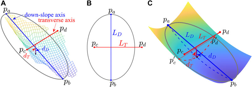
FIGURE 1. (A) The main (down-slope) axis and the transverse axis of a failure surface, which are perpendicular to each other in the top view and with depths, d_D and d_T, respectively. (B) The top view and the regressed ellipse. (C) The constructed idealized curved surface (ICS). It is noted that p_c and p_d lie at the scarp boundary, while $\overline{p_c^{\prime }{p}_d^{\prime }}$ denotes the minor axis of the reference ellipse.

2.2 Reference Ellipse and Construction of the ICS

Taylor et al. (2018) have pinpointed that an ellipse is a reasonably good approximation of the landslide shape, and a substantial percentage of historical landslides supports this conclusion. Although they did not distinguish the source and runout area (due to the employed inventories), significant deviations from the ellipse are found to be caused by the inclusion of the flow paths (channel morphology and merging of debris flows) or merges of several small landslides. In the present study, we propose to construct the ICS based on the reference ellipse, which fits the source area (or landslide-prone area identified by remote-sensing technology or/and field survey). The first step is to determine the major axis of the reference ellipse, and they connect the highest and lowest points (in elevation) of the (potential) source area. The second step is to determine the minor axis, which can be obtained by setting the area of the ellipse the same as the source area A_sa or by the width of the source area. In case only some morphological features or plausible failure locations/points are identified, the ellipse can be determined by regression with respect to these points.

An example is shown in Figure 2. Concerning the failure surface/area (Figure 2A), a reference ellipse is determined through the above elaborated two steps, where L₁ is the length of the major axis and L₂ is the length of the minor axis (Figure 2B). For a reference ellipse, each failure depth determines one ICS (see Figure 2C). The associated released mass volume can be calculated by the difference in the ICS and the pre-event topography through the digital elevation maps (DEMs). Once the released mass volume is given (e.g., by the volume–area relations), the sought ICS should yield nearly the same volume, and this can be achieved through iteration over a range of failure depths. It is obvious that the failure area determined by the ICS might deviate from the real/identified failure area; see Figure 2D. In the present study, it is suggested that the most appropriate ICS is the one that has minimal deviation to the failure area if the real failure area is available or the potential area is delineated. Hence, the determination of the reference ellipse plays a crucial role in constructing the ICS.

FIGURE 2

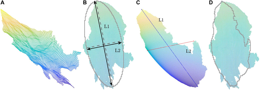
FIGURE 2. Main scarp area of the 2009 Hsiaolin landslide. (A) The failure surface. (B) Top view of the failure surface and the associated reference ellipse. (C) The constructed ICS. (D) Top view of the ICS (outlined) and failure surface (shaded, used in the SMS method).

The determination of the reference ellipse depends on the shape and orientation of the source area. However, the shapes of the source area are rather complex. Excluding highly irregular and branched shapes, we can approximately group the commonly observed shapes of landslide source area into five types (cf. Figure 3):

• Type I: Elliptical shape with major axis approximately in the down-slope direction.

• Type II: Elliptical shape with minor axis approximately in the down-slope direction.

• Type III: Ovate or lanceolate shape, of which the downstream part is wider.

• Type IV: Obovate or oblanceolate shape, of which the upstream part is wider.

• Type V: Concave hull, which can be seen as a distortion of the above types (Types I to IV).

FIGURE 3

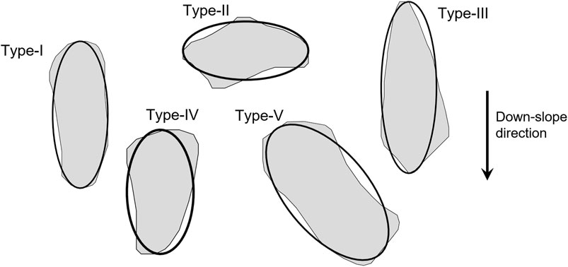
FIGURE 3. The commonly observed shapes of the landslide source area.

Types I, III, IV, and V cover the landslide shapes of Category D (more than 82% among 20,705 landslides) defined in the work of Taylor et al. (2018), while Type II is figured out from the inventory of rainfall-triggered landslides taking place in 2009 in Taiwan (cf. Lin et al., 2013; Tai et al., 2020). As listed in Table 1, four methods (A to D) are considered for abstracting the landslide source area of the five shape types to the reference ellipse. For distinguishing the down-slope axis L_D and transverse axis L_T of the source area, the lengths of the major and minor axes of the reference ellipse are denoted by L₁ and L₂, respectively, and its area is A_E. With the main axis $\overline{p_a{p}_b}$, one tries various reference ellipses by translation and rotation, i.e., setting the top vertex at the 48 grid points around p_a (i.e., ±3 grid points in the down- and cross-slope directions) and rotating with various angles (cf. Figure 4B). One should note that the vertices for the major/minor axis are assigned to be on the grid point of the digital elevation map (DEM), and its area is calculated with the mesh size. Hence, the length of the reference ellipse L₁ might not be equal to L_D exactly, and its area could slightly deviate from the area of source area A_sa in the searching process (i.e., one can only have L₁ ≈ L_D and A_E ≈ A_sa). Once the reference ellipse is fixed, each depth (d_D as shown in Figure 1A) determines one candidate ICS, yielding the associated released volume of mass as well as the failure area A_ICS. There are two criteria for figuring out the most appropriate ICS: 1) the released mass should be closest to the assigned one and 2) the minimum deviation of the resulted failure area A_ICS from the source area A_sa. Here, one should notice that the ICS-yielded failure area might be divided into several blocks due to the rugged topography, especially when the ICS tends to be flat. In the present study, the separated ones will be filtered out to alleviate the complexity.

TABLE 1

TABLE 1. Method of searching the optimal reference ellipse for constructing the most appropriate ICS.

FIGURE 4

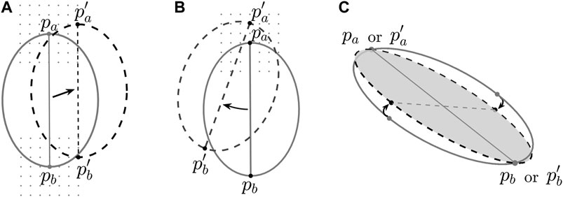
FIGURE 4. The location/orientation of the reference ellipse: (A) translation, (B) translation and rotation, and (C) side-tilting (only in method B).

Accordingly, under the prerequisite of the assigned volume of released mass (calculated by historical event or estimated by the volume–area relations), the four methods (A to D) are briefed in Table 1. In methods A and B, it is set that L₁ ≈ L_D and A_E ≈ A_sa, while the ellipse is allowed to tilt around its major axis in method B (cf. Figure 4C). With L₁ ≈ L_D, various reference ellipses of different values for L₂ are tested for constructing the candidate ICSs in method C, while the ellipse area A_E does not remain invariant (due to the different values of L₂). Accompanied with various values of L₂ but keeping A_E ≈ A_sa, the magnitude of L₁ co-varies in method D. That is, the shape of the reference ellipse is fixed in methods A and B. In methods C and D, the shapes of the reference ellipse are variable, while the ellipse area A_E remains invariant in method D. In addition, it has to be noted that the translation and rotation procedures are performed in the searching process in all of the four methods, while only in method B, the reference ellipse is allowed to tilt around its major axis (cf. Figure 4C).

In this ellipse–ICS approach, the major axis of the reference ellipse generally lies along the down-slope direction (for shapes of Type I, III, IV, or V). For shapes of Type II, the minor axis is assigned to follow the down-slope direction with the major axis lying in the transverse direction because its transverse extension is wider than the one in the down-slope direction. As will be detailed in the following section, the present approach (through methods A to D) is able to deliver appropriate ICSs, of which the resulted failure area may serve as a reasonable approximation to the (assigned) source area.

3 Application to a Historical Event and Landslide-prone Areas

The proposed methods (method A to D) for constructing the most appropriate ICS are applied to a historical landslide event and one landslide-prone area. The historical event is the Hsiaolin landslide occurred in 2009 in southern Taiwan. As a representative event in Taiwan, it has received significant research interests and we would refer the readers for details to the relevant literature, such as the work of Dong et al. (2011), Kuo et al. (2011), Tai et al. (2019), and Tai et al. (2020). In application to the Hsiaolin landslide, we only consider the main scarp area, marked by HL-1 as shown in Figure 5, which consists of more than 94% landslide mass as given in the work of Kuo et al. (2011) and Tai et al. (2019).

FIGURE 5

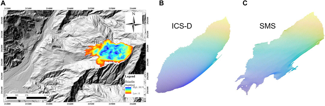
FIGURE 5. (A) The main scar area (HL-1) of the Hsiaolin landslide event. (B) The constructed ICS for HL-1 by method D. (C) The surface determined by the smooth minimal surface (SMS) method proposed in Kuo et al. (2020).

For the landslide-prone areas, we consider a potential large-scale landslide area, named Taitung-Yanping-T003, which locates near Wu-Ling village in the Luliao watershed in Taitung county, south-eastern Taiwan (cf. Lai, 2019; Wang, 2020). As elaborated in the report (Wang, 2020), the plausible outline of a large-scale deep-seated landslide of potential in this area was delineated (by the high-resolution DEMs together with field survey); see the red line marked area in Figure 6A. Also, comprehensive LiDAR image interpretation and topography analysis reveal three unstable blocks (W-1, W-2, and W-3) in plausible movement, outlined by yellow lines. Besides, many cracks are identified and depicted by red curves with bulges and the light-yellow railing areas indicate the dip slopes. For disaster monitoring and risk management, two gaging wells with inclinometers (at the middle of W-1 and W-2) are set up to monitor the groundwater level, potential failure surface, and the movement of the blocks (cf. Lai, 2019; Wang, 2020). The green circle markers (BW-I and BW-II) in Figure 6A indicate their locations, respectively. Figure 6B shows the records of these gaging wells. A definite sliding surface is detected at the depth between 16 and 17 m from the ground surface at BW-I, and the groundwater level lies at 26.8 m deep. The monitoring records of BW-II reveals that the groundwater is ca. 17.8 m deep and the sliding surface lies in the range of [24, 25] m deep. Identifying the landslide-prone area is based on geomorphological features, and the delineation of the boundary highly depends on personal experiences. These measurements provide an excellent example for re-examining the applicability of the current delineation and the associated planned mitigation countermeasure. Here, the employment of ICSs may provide plausible scenarios as useful reference information. Besides, the plausible failure surface, constructed by the volume-constrained smooth minimal surface (SMS) method (Kuo et al., 2020), is also considered and evaluated in this campaign, if applicable.

FIGURE 6

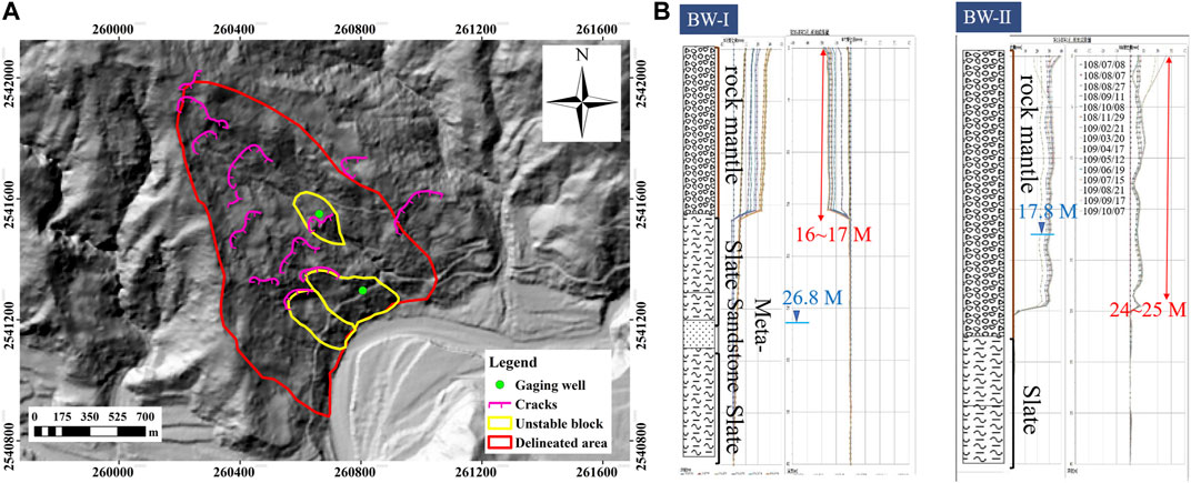
FIGURE 6. (A) The hillshade map of Taitung-Yanping-T003, where the red line outlines the suspected landslide-prone area, the yellow lines indicate three blocks plausibly in movement, the cracks are depicted by red curves with bulges, and the light-yellow railing areas represent the dip slopes. (B) The monitoring records of gaging wells BW-I and BW-II.

By constructing the ICS, the expected released volume V_ICS should be given in advance. For historical events, V_ICS is set to be approximately equal to the exact landslide volume V_LS. For landslide-prone areas, the value of V_ICS can be set by empirical volume–area relations. In the present study, the Guzzetti (2009)relation is employed because the considered landslides are also in sliding type, and this relation may provide sound agreement with the ones in Taiwan (see the work of Tai et al., 2020). One may choose some other appropriate empirical relations as well, if applicable. In the searching process with the four methods (methods A to D), thousands of reference ellipses and their associated ICSs are constructed. The performance of each ICS is evaluated in terms of four indices, $\left({\lambda }_E,{\mathrm{\Lambda }}_E,{\lambda }_S,{\mathrm{\Lambda }}_S\right)$, as defined and listed in Table 2. λ_E denotes the difference between the reference ellipse A_E and the source area A_sa. It should be near zero in methods A, B, and D (cf. Table 1). Λ_E stands for the deviated area of coverage. λ_S and Λ_S are for the resulted failure area A_ICS and the source area A_sa, where Λ_S represents the deviation index of area coverage. The most appropriate ICS is the one with the minimal difference between the covered area of A_ICS and A_sa (i.e., the one with the minimal value of the deviation index of area coverage Λ_S). In case the values of Λ_S of two ICSs are very close, the one with the smallest value of λ_S + Λ_S is chosen as the most appropriate ICS (see, e.g., Scenario I in Table 4).

TABLE 2

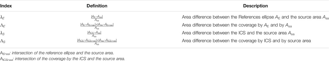
TABLE 2. Indices for evaluating the performance of methods for constructing the ICS.

In addition to searching the most appropriate ICS, numerical simulations are performed with the ICSs determined in various scenarios to investigate the impacts on the flow paths when the landslide takes place (e.g., hazard assessment). As a large portion of the hazardous landslides in Taiwan are triggered by heavy rainfall, the two-phase model for non-trivial topography (Tai et al., 2019) is employed here. In addition, the code has been reprogrammed and implemented for CUDA-GPU high-performance computation (MoSES_2PDF, see the work of Ko et al., 2021). For minimizing the uncertainty and for a unique reference, all the parameters are set identical to the ones used in the work of Tai et al. (2019). We refer readers to the work of Tai et al. (2019) and Ko et al. (2021) for details of the model equations and the applied GPU techniques used in the simulation tool, respectively. Besides, only the areas covered by flow depth more than 10 cm are taken into account in investigating the flow paths.

3.1 The 2009 Hsiaolin Landslide

Only the main source area (HL-1, in Figure 5A) by the 2009 Hsiaolin landslide is considered in this campaign, where the four methods (A, B, C, and D) are employed for constructing the ICSs. The area of the main scar (HL-1) is 624,900 m² with a mass volume of 21, 180, 535 m³, where a 10 m resolution digital elevation map (DEM) is used. After the process of looking for the optimal reference ellipse (translation, rotations, and tilting as listed in Table 1) to construct the most appropriate ICS, Table 3 shows the results of the four methods (A, B, C, and D) with respect to the four Indices $\left({\lambda }_E,{\mathrm{\Lambda }}_E,{\lambda }_S,{\mathrm{\Lambda }}_S\right)$. It is found that these four methods can provide reasonable ICSs that are with a deviation of coverage less than 30% (i.e., Λ_S < 0.3). Although the ICS made by method C is with the least deviation in terms of coverage (Λ_S), the ICS area by method D is closest to the scarp area. When searching for the most appropriate ICS, one can choose the one with the smallest value of Λ_S or the sum λ_S + Λ_S.

TABLE 3

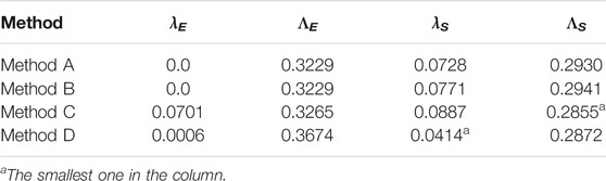
TABLE 3. Performance indices with regard to the most appropriate ICS constructed by the four methods for HL-1 (2009 Hsiaolin landslide event).

To investigate the impacts of the plausible failure surface on the flow paths, we take the one constructed by method D as the most appropriate ICS (denoted by ICS-D) in the computation. Besides, the plausible failure surface determined by the smooth minimal surface (SMS) method is also considered in this campaign. The 3D illustrations of the ICS-D and SMS are given in Figures 5B,C, respectively, and their outlines (top view) are depicted in Figure 2D. In both cases, the simulation ends at t = 181.83 s when all the masses are nearly at the state of rest. Figure 7 shows the flow paths computed with ICS-D and the one constructed by the SMS method (denoted by SMS), where the areas with flow thickness less than 10 cm are filtered out. The area in cyan indicates the paths in both simulations, the magenta area is covered only by the ICS-D computation, and the yellow area is only in the scenario of the SMS method. Although the deviation index of coverage Λ_S reaches 0.2872, the differences between the flow paths are around 14.3%, i.e., ca. 85.7% of the total flow paths are overlapped. The main differences are found to be on the flanks of the source area (HL-1), and it is suspected to be mainly caused by the different outline/coverage between ICS-D and SMS. That is, deviation occurs at the first period when the mass is released and starts to slide. In the subsequent stage, most of the moving mass flows into a channelized topography so that the geometry of the failure surface does not have significant impacts on the following paths anymore.

FIGURE 7

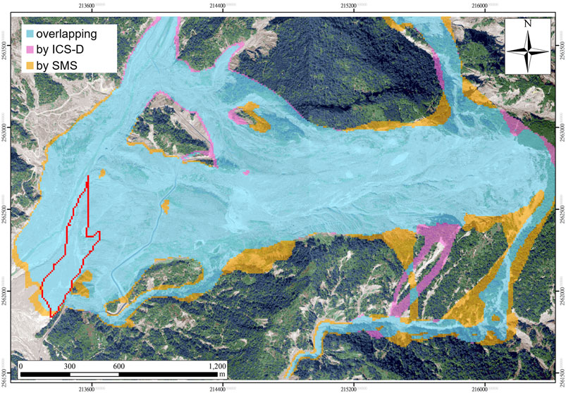
FIGURE 7. Difference in the flow paths computed with the ICS-D and the smooth minimal surface method (SMS method), where the magenta area indicates the paths only by the ICS-D, the yellow area denotes the area only the SMS surface, and the cyan means the common flow paths during the simulation period (from t = 0 s to t = 181.83 s). The Hsiaolin village is depicted by the red contour. (Orthophoto: Courtesy of Aerial Survey Office, Forestry Bureau, Taiwan).

3.2 The Landslide-Prone Area (Taitung-Yanping-T003)

The area of the landslide-prone area (Taitung-Yanping-T003) reads 515,900 m², with which the volume–area relation, suggested by Guzzetti et al. (2009), yields a plausible volume of released mass by 15, 565, 651 m³. The resolution of the used digital elevation map (DEM) is 5 m. In terms of the delineated landslide-prone area and the three unstable blocks, five scenarios are assigned as listed in Table 4. Scenarios I and II are the individual releases of blocks W-1 and W-2, respectively. Blocks W-1 and W-3 are supposed to be released simultaneously in Scenario III. In Scenario IV, it is supposed that the landslide scarp follows the delineated outline. Scenario V is to figure out the most plausible failure scarp determined by the ellipse–ICS method, which covers all the cracks and the three unstable blocks within the delineated area, and the predicted failure depths are close to the records of the gaging well. The sketches of the scenarios are given in Supplementary Image 1. In all the scenarios (I to V), the associated volumes of released mass are calculated by Guzzetti’s law (Guzzetti et al., 2009). Since the boundaries of the delineated areas are precisely given in Scenarios I to IV, the SMSs are also constructed for comparison.

TABLE 4

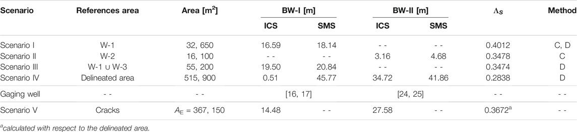
TABLE 4. Scenarios for Taitung-Yanping-T003.

Table 4 lists the results of the most appropriate ICSs and SMSs with respect to the assigned areas, where the failure depths at the locations of BW-II and BW-I are the averaged values over the neighboring grids (9 grids in total) in the DEM. In Scenario I (for block W-1), both methods C and D (abbreviated by ICS-C and ICS-D, respectively) yield the ICSs with approximately the same deviation index of coverage Λ_S and we choose ICS-C as the most appropriate ICS for its slightly better performance by λ_S. Although the value of Λ_S by ICS-C reaches 0.4012, the associated failure depth lies at 16.59 m, exactly in the range of the inclinometer records (BW-I). On the other hand, the depth of the failure surface determined by the SMS reads 18.14 m, slightly deeper as indicated by the inclinometer (BW-I). Both predictions (by ICS-C and SMS) support the delineation of the unstable block W-1. In Scenario II (block W-2), both ICS and SMS predict the failure depths less than 5 m (3.16 and 4.68 m, respectively), which is far away from the records (in the range [24, 25]). This finding indicates that the delineation of unstable block W-2 could be questionable or more investigation seems needed. In Scenario III, predictions of ICS and SMS for the failure depth are 19.50 and 20.84 m, respectively, slightly more than the records. Since the volumes of landslide mass in scenarios I and III are estimated by the empirical volume–area relation (Guzzetti et al., 2009), the coincidence of the failure depth indicates the high possibility for these two scenarios.

The results of scenarios IV and V are shown in Figure 8, in which the left panels (a, b, and c) depict Scenario IV and the right panels (d, e, and f) are for Scenario V. In panels a and d, the delineated area is depicted by red contour, and the ICS-resulted failure areas are marked by jade-green shade for scenarios IV and V, respectively. The employed reference ellipses for constructing the ICSs are shown by red-outlines in panels b and e, while the depth distributions of plausible release mass are given in panels c and f for scenarios IV and V, respectively. In Scenario IV, where the delineated area (the red-outlined area in panel a or the blue-shaded area in panel b) serves as the source area A_sa in the searching process, the most appropriate ICS is constructed by method D (denoted by ICS-D). As listed in Table 4, the ICS-D predicts the failure depths of 0.51 m for BW-I and 34.72 m for BW-II, while they are 45.77 and 41.86 m, respectively, for the SMS. With respect to the inclinometer records [16, 17] m and [24, 25] m, the predicted depths are far too deep, although the ICS-D covers nearly the same area except for the south-eastern part (cf. panel a) where the deviation index of coverage Λ_S = 0.2838. This deviation reveals that the present ellipse–ICS method seems inapplicable to Scenario IV, or the whole delineated area’s failure would not take place at one time. Relating the inclinometer records with the plausible failure depths, we relax the constraint of the delineated area and suppose that all the cracks within the delineated area are induced by the same landslide body to be released (Scenario V). With the released volume (calculated by the Guzzetti (2009)law), the computed ICS suggests the failure depths of 14.48 m for BW-I and 27.58 m for BW-II (cf. the bottom row of Table 4). That is, in Scenario V, both depths predicted by ICS are close to the ones recorded by inclinometers. As shown in Figure 8D, the range of ICS is approximately in agreement with the delineated area in the upper part. This finding suggests a plausible failure area and its associated released volume of mass when the cracks and both records of the two gaging wells are taken into account. It indicates the practicality of the proposed ellipse–ICS approach, that it is able to deliver approximately reasonable estimation even when a precise delineation of the landslide-prone area is missing.

FIGURE 8

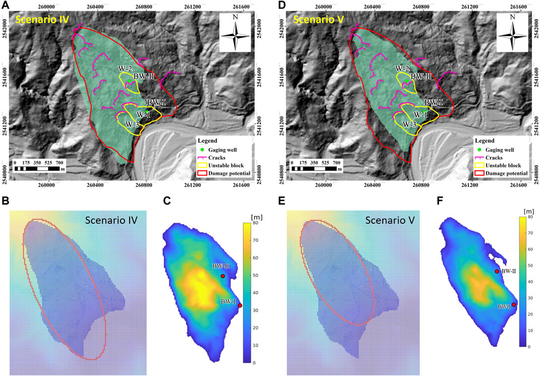
FIGURE 8. Scenarios IV and V (Taitung-Yanpin-T003). (A,D) The covered area by the computed ICS (shaded in jade-green), the delineated landslide-prone area (red contour), and the locations of gaging wells (BW-I and BW-II). (B,E) The delineated landslide-prone area (blue shade) and the reference ellipse (red outlined) for constructing the most appropriate ICS. (C,F) Depth distribution of the released mass with respect to the ICS.

Based on the above scenario investigations, scenarios I, III, and V could be possible situations. Numerical simulations are therefore performed in terms of the scenarios for investigating the flow paths, where the simulation tool MoSES_2PDF (Ko et al., 2021) is employed. Figure 9A illustrates the flow paths of scenarios IV and V, where only the areas covered by flow thickness more than 10 cm are shown. The cyan area means the common flow paths in both scenarios, and the brown area is marked only in Scenario IV. Although the landslide mass (based on Guzzetti’s (2009) empirical relation) in Scenario IV is about 1.6-fold to Scenario V, the traveling distance (along the down-slope direction) does not significantly increase compared to the one in Scenario V. The main difference lies in the lateral direction and is suspected to be induced by the discrepancies of the source area and by the different released volume. In both scenarios (IV and V), the landslide mass does not reach the Wu-Ling village located south-eastern from the landslide area. We also considered two small-scale plausible cases for the three unstable blocks (W-1, W-2, and W-3). In the first case, the three blocks are released simultaneously (simultaneous release). In the second case, the lower blocks (W-1 and W-3) are released first, followed by the release of W2 (sequential failure). Figure 9B presents the computed flow paths of these two cases. Similar to panel a, the cyan area indicates the common flow paths in both cases. The brown area is covered only in the first case (simultaneous release), and the fuchsia area is marked only in the second case (sequential failure). Interestingly, the sequential release yields nearly the same traveling distance but flow paths cover a larger area. Although the area expansion is around 5.2%, one has to pay attention to the impacts of a possible sequential failure by risk analysis or hazard assessment.

FIGURE 9

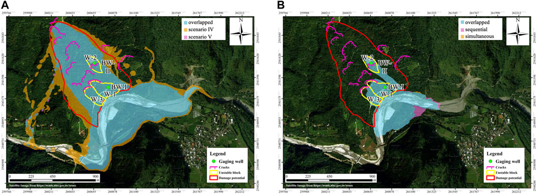
FIGURE 9. (A) Flow paths in scenarios IV and V. (B) Flow paths by a simultaneous release of the three unstable blocks (W-1, W-2, and, W-3) or by sequential failure (Orthophoto: Courtesy of National Land Surveying and Mapping Center, Taiwan).

4 Concluding Remarks

This work outlines a methodology to systematically estimate the plausible landslide failure area, the associated volume of released mass, and the subsequent flow paths when the failure in an area of landslide susceptibility takes place. This method employs the concept of reference ellipse for constructing the idealized curved surface (ICS). Through translation, rotation, and side-tilting of the reference ellipse, there are thousands of ellipses (orientations) to be assessed. Together with the assigned failure depth, the constructed ICS cuts the local topography and yields the plausible failure area as well as the volume of mass to be released. Each ellipse is associated with one candidate ICS, which yields the volume of released mass as assigned (calculated by historical events or empirical volume–area relations). The most appropriate ICS is the one with the minimal deviation of the coverage between the ICS–resulted failure area and the delineated area (or the source area in historical events). As a matter of course, this approach would demand more computational resources. Nevertheless, it is an economical compromise because it does not request the expensive and time-consuming data obtained from geologic drilling, analysis of geological structure or comprehensive field survey, etc. No conflict exists. This ellipse–ICS approach can benefit from the field data (spatial geological variations, hydrological conditions, weathering effects, etc.) for its reliability. or reversely, the present ellipse–ICS approach may provide helpful information, such as the appropriate locations of gaging stations.

We investigate the feasibility and practicability of the ellipse–ICS approach by application to the 2009 Hsiaolin landslide (historical event) and the delineated landslide-prone area (Taitung-Yanping-T003). The plausible failure surfaces determined by the SMS method (Kuo et al., 2020) are included in the campaign if a precise delineation of the source area is available. Since the SMS method requests a precise boundary of the source area, the difference in the flow paths between ICS and SMS clarifies the impacts of the geometry of the released mass on the flow paths. By simulating the 2009 Hsiaolin landslide, more than 85% of the flow paths are overlapped, although the deviation index of coverage Λ_S between ICS and SMS reaches ca. 0.29. For the landslide-prone area (Taitung-Yanping-T003), five scenarios are arranged for mimicking plausible failure surface by ICS that agrees with the inclinometer records. This scenario investigation also highlights the characteristic that the ellipse–ICS method is applicable without a concrete delineated area. Combining the ellipse–ICS approach and the GPU-based simulation package provides an optimal tool for hazard assessment in various scenarios. The released volume of mass is estimated, and the subsequent flow paths are predicted.

It has to be noted that the present ellipse–ICS approach is based on the geomorphological concept, and it mimics the plausible failure surface by a smooth surface. It is certainly not intended to replace the conventional stability analysis. Instead, it fills the vacancy of the conventional analytical tools when only limited spatial, geological, and hydrological data are available. However, it works at the expense of computational resources that the most appropriate ICS is figured out among the thousands of reference ellipse and the associated candidate ICSs. In Scenario IV, there are 1,519 reference ellipses to be evaluated in methods A and B, while 10,633 reference ellipses in methods C and D. For each reference ellipse, one has to determine the depth to match the assigned volume of release mass utilizing iteration. A normal PC (i7-8700 CPU@3.20 GHz, 16 GB memory, Linux OS) takes about one to several hours to figure out the most appropriate ICS for one case/scenario. One possible way to enhance the computational efficiency is implementing the genetic algorithm (GA) (e.g., Whitley, 1994) together with GPU-accelerated computation for the current ellipse–ICS approach. We are working on it and will report the updates in due time.

Data Availability Statement

The data analyzed in this study are subject to the following licenses/restrictions: It is remarked that, following the government regulation, only the DEMs with a resolution of 20 × 20 m can be provided. The interpolated ones, not exactly identical to the ones used in the study, are available on request to the corresponding author. Requests to access these datasets should be directed to Y-CT, yctai@ncku.edu.tw.

Author Contributions

C-JK, C-LW, and H-KW: data analysis and numerical simulation. W-CL and C-YK: concept/opinion exchange and content confirmation. Y-CT: idea, design of the work, and construction of the MS. All authors contributed to the article and approved the submitted version.

Funding

The financial support of the Ministry of Science and Technology, Taiwan (MOST 109-2221-E-006-022),and the Soil and Water Conservation Bureau, Council of Agriculture, Taiwan (SWCB-109-269) are acknowledged.

Conflict of Interest

The authors declare that the research was conducted in the absence of any commercial or financial relationships that could be construed as a potential conflict of interest.

Publisher’s Note

All claims expressed in this article are solely those of the authors and do not necessarily represent those of their affiliated organizations, or those of the publisher, the editors and the reviewers. Any product that may be evaluated in this article, or claim that may be made by its manufacturer, is not guaranteed or endorsed by the publisher.

Supplementary Material

The Supplementary Material for this article can be found online at: https://www.frontiersin.org/articles/10.3389/feart.2021.733413/full#supplementary-material

References

Bishop, A. W. (1955). The Use of the Slip circle in the Stability Analysis of Slopes. Géotechnique 5, 7–17. doi:10.1680/geot.1955.5.1.7

CrossRef Full Text | Google Scholar

Briaud, J.-L. (2013). Geotechnical Engineering: Unsaturated and Saturated Soils. Hoboken, New Jersey: John Wiley & Sons.

Delbridge, B. G., Bürgmann, R., Fielding, E., Hensley, S., and Schulz, W. H. (2016). Three-Dimensional Surface Deformation Derived From Airborne Interferometric UAVSAR: Application to the Slumgullion Landslide. J. Geophys. Res. Solid Earth. 121, 3951–3977. doi:10.1002/2015jb012559

CrossRef Full Text | Google Scholar

Dong, J.-J., Li, Y.-S., Kuo, C.-Y., Sung, R.-T., Li, M.-H., Lee, C.-T., et al. (2011). The Formation and Breach of a Short-Lived Landslide Dam at Hsiaolin Village, Taiwan - Part I: Post-Event Reconstruction of Dam Geometry. Eng. Geology 123, 40–59. doi:10.1016/j.enggeo.2011.04.001

CrossRef Full Text | Google Scholar

Fellenius, W. (1927). Swedish Slice Method Calculations With Friction and Cohesion Under the Assumption of Cylindrical Sliding Surfaces (Erdstatische Berechnungen mit Reibung und Kohäsion (Adhäsion) und Unter Annahme kreiszylindrischer Gleitflächen). Berlin: Verlag Ernst and Sohn Press.

GEO-SLOPE International Ltd (2012). Stability Modeling with SLOPE/W. Calgary, Alberta, Canada: GEO-SLOPE International Ltd.

Griffiths, D. V., and Lane, P. A. (1999). Slope Stability Analysis by Finite Elements. Géotechnique 49, 387–403. doi:10.1680/geot.1999.49.3.387

CrossRef Full Text | Google Scholar

Guzzetti, F., Ardizzone, F., Cardinali, M., Rossi, M., and Valigi, D. (2009). Landslide Volumes and Landslide Mobilization Rates in Umbria, Central Italy. Earth Planet. Sci. Lett. 279, 222–229. doi:10.1016/j.epsl.2009.01.005

CrossRef Full Text | Google Scholar

Huang, C.-C., Tsai, C.-C., and Chen, Y.-H. (2002). Generalized Method for Three-Dimensional Slope Stability Analysis. J. Geotech. Geoenviron. Eng. 128, 836–848. doi:10.1061/(asce)1090-0241(2002)128:10(836)

CrossRef Full Text | Google Scholar

Huang, C.-C., and Tsai, C.-C. (2000). New Method for 3D and Asymmetrical Slope Stability Analysis. J. Geotech. Geoenviron. Eng. 126, 917–927. doi:10.1061/(asce)1090-0241(2000)126:10(917)

CrossRef Full Text | Google Scholar

Iverson, R. M., George, D. L., Allstadt, K., Reid, M. E., Collins, B. D., Vallance, J. W., et al. (2015). Landslide Mobility and Hazards: Implications of the 2014 Oso Disaster. Earth Planet. Sci. Lett. 412, 197–208. doi:10.1016/j.epsl.2014.12.020

CrossRef Full Text | Google Scholar

Jaboyedoff, M., Baillifard, F., Couture, R., Locat, J., Locat, P., and Rouiller, J. (2004). “New Insight of Geomorphology and Landslide Prone Area Detection Using Digital Elevation Model(s),” in Landslides Evaluation and Stabilization. Editors W. Lacerda, M. Ehrlich, A. Fontoura, and A. Sayo (Rotterdam: Balkema), 191–197. doi:10.1201/b16816-26

CrossRef Full Text | Google Scholar

Jaboyedoff, M., Chigira, M., Arai, N., Derron, M.-H., Rudaz, B., and Tsou, C.-Y. (2019). Testing a Failure Surface Prediction and Deposit Reconstruction Method for a Landslide Cluster that Occurred During Typhoon Talas (Japan). Earth Surf. Dynam. 7, 439–458. doi:10.5194/esurf-7-439-2019

CrossRef Full Text | Google Scholar

Jaboyedoff, M., Couture, R., and Locat, P. (2009). Structural Analysis of Turtle Mountain (Alberta) Using Digital Elevation Model: Toward a Progressive Failure. Geomorphology 103, 5–16. doi:10.1016/j.geomorph.2008.04.012

CrossRef Full Text | Google Scholar

Janbu, N. (1973). “Slope Stability Computations,” in Embankment-dam Engineering, Casaggrande Volume (New York: Wiley), 47–86.

Google Scholar

Janbu, N. (1954). Stability Analysis for Slopes with Dimensionless Parameters. Ph.D. Thesis. Cambridge, Massachusetts: Harvard University.

Ko, C.-J., Chen, P.-C., Wong, H.-K., and Tai, Y.-C. (2021). MoSES_2PDF: A GIS-Compatible GPU-Accelerated High-Performance Simulation Tool for Grain-Fluid Shallow Flows. arXiv preprint arXiv:2104.06784 [cs.CE]

Google Scholar

Kuo, C.-Y., Tsai, P.-W., Tai, Y.-C., Chan, Y.-H., Chen, R.-F., and Lin, C.-W. (2020). Application Assessments of Using Scarp Boundary-Fitted, Volume Constrained, Smooth Minimal Surfaces as Failure Interfaces of Deep-Seated Landslides. Front. Earth Sci. 8, 211. doi:10.3389/feart.2020.00211

CrossRef Full Text | Google Scholar

Kuo, C., Tai, Y.-C., Chen, C., Chang, K., Siau, A., Dong, J., et al. (2011). The Landslide Stage of the Hsiaolin Catastrophe: Simulation and Validation. J. Geophys. Res. Earth Surf. 116, F04007. doi:10.1029/2010jf001921

CrossRef Full Text | Google Scholar

Lai, W.-J. (2019). Disaster Investigation and Countermeasure Strategy of Luliao Watershed (Taitung-Yanping-D002 Potential Large-Scale Landslide and Kanaluk Area)(in Chinese). Taiwan: Tech. rep., Soil and Water Conservative Bureau, Council of Agriculture. Rep.-No.: SWCB-108-127.

Lam, L., and Fredlund, D. G. (1993). A General Limit Equilibrium Model for Three-Dimensional Slope Stability Analysis. Can. Geotech. J. 30, 905–919. doi:10.1139/t93-089

CrossRef Full Text | Google Scholar

Larsen, I. J., Montgomery, D. R., and Korup, O. (2010). Landslide Erosion Controlled by Hillslope Material. Nat. Geosci. 3, 247–251. doi:10.1038/ngeo776

CrossRef Full Text | Google Scholar

Lin, C.-W., Chang, W.-S., Liu, S.-H., Tsai, T.-T., Lee, S.-P., Tsang, Y.-C., et al. (2011). Landslides Triggered by the 7 August 2009 Typhoon Morakot in Southern Taiwan. Eng. Geology 123, 3–12. doi:10.1016/j.enggeo.2011.06.007

CrossRef Full Text | Google Scholar

Lin, C.-W., Tseng, C.-M., and Chen, R.-F. (2013). Survey and Assessment of Potential Large-Scale Landslides Hazards in Mountainous Areas of Kao-Ping River Watershed. Taiwan: Tech. rep., Soil and Water Conservative Bureau, Council of Agriculture.

Morgenstern, N. R., and Price, V. E. (1965). The Analysis of the Stability of General Slip Surfaces. Géotechnique 15, 79–93. doi:10.1680/geot.1965.15.1.79

CrossRef Full Text | Google Scholar

Reid, M. E., Christian, S. B., and Brien, D. L. (2000). Gravitational Stability of Three-Dimensional Stratovolcano Edifices. J. Geophys. Res. 105, 6043–6056. doi:10.1029/1999jb900310

CrossRef Full Text | Google Scholar

Reid, M. E., Christian, S. B., Brien, D. L., and Henderson, S. (2015). Scoops3D–Software to Analyze Three-Dimensional Slope Stability Throughout a Digital Landscape. Menlo Park, CA, USA: US Geological Survey; Volcano Science Center.

Reid, M. E., Sisson, T. W., and Brien, D. L. (2001). Volcano Collapse Promoted by Hydrothermal Alteration and Edifice Shape, Mount Rainier, Washington. Geol. 29, 779–782. doi:10.1130/0091-7613(2001)029<0779:vcpbha>2.0.co;2

CrossRef Full Text | Google Scholar

Sala, G., Lanfranconi, C., Frattini, P., Rusconi, G., and Crosta, G. B. (2021). Cost-Sensitive Rainfall Thresholds for Shallow Landslides. Landslides 18, 2979–2992. doi:10.1007/s10346-021-01707-4

CrossRef Full Text | Google Scholar

Shen, H., and Abbas, S. M. (2013). Rock Slope Reliability Analysis Based on Distinct Element Method and Random Set Theory. Int. J. Rock Mech. Mining Sci. 61, 15–22. doi:10.1016/j.ijrmms.2013.02.003

CrossRef Full Text | Google Scholar

Stumpf, A., Malet, J.-P., Kerle, N., Niethammer, U., and Rothmund, S. (2013). Image-Based Mapping of Surface Fissures for the Investigation of Landslide Dynamics. Geomorphology 186, 12–27. doi:10.1016/j.geomorph.2012.12.010

CrossRef Full Text | Google Scholar

Tai, Y.-C., Ko, C.-J., Li, K.-D., Wu, Y.-C., Kuo, C.-Y., Chen, R.-F., et al. (2020). An Idealized Landslide Failure Surface and its Impacts on the Traveling Paths. Front. Earth Sci. 8, 313. doi:10.3389/feart.2020.00313

CrossRef Full Text | Google Scholar

Tai, Y. C., Heß, J., and Wang, Y. (2019). Modeling Two‐Phase Debris Flows With Grain‐Fluid Separation Over Rugged Topography: Application to the 2009 Hsiaolin Event, Taiwan. J. Geophys. Res. Earth Surf. 124, 305–333. doi:10.1029/2018jf004671

CrossRef Full Text | Google Scholar

Taylor, F. E., Malamud, B. D., Witt, A., and Guzzetti, F. (2018). Landslide Shape, Ellipticity and Length-To-Width Ratios. Earth Surf. Process. Landforms 43, 3164–3189. doi:10.1002/esp.4479

CrossRef Full Text | Google Scholar

Tran, T. V., Alvioli, M., and Lee, G. (2018). Three-Dimensional, Time-Dependent Modeling of Rainfall-Induced Landslides Over a Digital Landscape: a Case Study. Landslides 15, 1071–1084. doi:10.1007/s10346-017-0931-7

CrossRef Full Text | Google Scholar

Van Tien, P., Trinh, P., Luong, L., Nhat, L., Duc, D., Hieu, T., et al. (2021). The October 13, 2020, Deadly Rapid Landslide Triggered by Heavy Rainfall in Phong Dien, Thua Thien Hue, Vietnam. Landslides 18, 2329–2333. doi:10.1007/s10346-021-01663-z

CrossRef Full Text | Google Scholar

Wang, P.-C. (2020). FY 109 Field Survey and Monitoring for Large-Scale Landslide in Taitung County (In Chinese). Taiwan: Tech. rep., Soil and Water Conservative Bureau, Council of Agriculture. Rep.-No.: SWCB-109-080.

Whitley, D. (1994). A Genetic Algorithm Tutorial. Stat. Comput. 4, 65–85. doi:10.1007/bf00175354

CrossRef Full Text | Google Scholar

Yeh, C.-H., Dong, J.-J., Khoshnevisan, S., Juang, C. H., Huang, W.-C., and Lu, Y.-C. (2021). The Role of the Geological Uncertainty in a Geotechnical Design - A Retrospective View of Freeway No. 3 Landslide in Northern Taiwan. Eng. Geology 291, 106233. doi:10.1016/j.enggeo.2021.106233

CrossRef Full Text | Google Scholar

Zhang, L., Li, J., Li, X., Zhang, J., and Zhu, H. (2018). Rainfall-induced Soil Slope Failure: Stability Analysis and Probabilistic Assessment. Boca Raton, FL: CRC Press.

Zhang, S., and Wang, F. (2019). Three-Dimensional Seismic Slope Stability Assessment With the Application of Scoops3D and GIS: a Case Study in Atsuma, Hokkaido. Geoenviron. Disasters 6, 9. doi:10.1186/s40677-019-0125-9

CrossRef Full Text | Google Scholar