Least-Squares Reverse Time Migration Using the Gradient Preconditioning Based on Transmitted Wave Energy

A gradient preconditioning approach based on transmitted wave energy for least-squares reverse time migration (LSRTM) is proposed in this study. The gradient is preconditioned by using the energy of “approximate transmission wavefield,” which is calculated based on the non-reflecting acoustic equation. The proposed method can effectively avoid a huge amount of calculation and storage required by the Hessian matrix or approximated Hessian matrix and can overcome the influence of reflected waves, multiples, and other wavefields on the gradient in gradient preconditioning based on seismic wave energy (GPSWE). The numerical experiments, compared with that using GPSWE, show that LSRTM using the gradient preconditioning based on transmitted wave energy (GPTWE) can significantly improve the imaging accuracy of deep target and accelerate the convergence rate without trivial increased calculation.

Introduction

Compared with traditional migration techniques such as Kirchhoff integral migration, reverse time migration (RTM) based on the two-way wave equation is widely favored by researchers (Baysal et al., 1983; McMechan, 1983; Yoon and Marfurt, 2006; Symes, 2007; Fletcher et al., 2009; Liu et al., 2011; Sun et al., 2016) because of its obvious advantages in accurate imaging of complex media (especially high-steep structure and subsalt structure). However, RTM still belongs to the category of conventional migration, and its migration operator is the conjugate transposition of the forward-modeling operator, rather than the exact inverse operator (Claerbout, 1992). Therefore, conventional RTM produces blurring imaging of underground media under the influence of factors such as a complex structure, limited bandwidth, and under-sampled acquisition system, which is difficult to satisfy the current needs of oil and gas exploration and development (Nemeth et al., 1999).

Dai et al. (2010) regarded the conventional RTM as an inversion problem under the framework of least squares, used the iterative method to obtain the reflection coefficient model, and developed a least-squares reverse time migration (LSRTM) method. Since the LSRTM can obtain the imaging results with high precision, high-amplitude preservation, and high resolution, it has become a research hotspot in the field of geophysics (Dai et al., 2012; Guo and Li, 2014; Huang et al., 2014; Yao and Jakubowicz, 2016; Ren et al., 2017; Rocha and Sava, 2018; Gong et al., 2019; Yang et al., 2019; Yang and Zhu, 2019; Li et al., 2020). Dai et al. (2012) proposed multisource LSRTM based on phase encoding, which improved the computational efficiency of the algorithm. Guo and Li (2014) implemented the true-amplitude imaging based on LSRTM and obtained the imaging with high resolution and true amplitude. Huang et al. (2014) achieved high-precision imaging of near surfaces based on LSRTM. Wong et al. (2015) proposed a joint LSRTM method by using primary and free-surface multiples and attenuated crosstalk artifacts in the image. Yao and Jakubowicz (2016) developed the LSRTM in a matrix-based formulation, which could obtain the high-precision section on the basis of effectively suppressing artifacts. Ren et al. (2017) developed elastic LSRTM, which provided more abundant and effective information for accurate imaging of complex media. Rocha and Sava (2018) proposed elastic LSRTM using the energy norm to improve imaging accuracy and speed up the convergence. Gong et al. (2019) applied a sparsity-promoting constraint to the LSRTM and obtained better imaging, especially for the metallogenetic geological model containing small-scale scatters. Yang et al. (2019) used a high-order Born approximation algorithm to supplement the information of prismatic waves in conventional LSRTM and further enhanced the ability to finely characterize the steeply dipping structure. Yang and Zhu (2019) implemented a viscoacoustic LSRTM based on a time-domain complex-valued wave equation, which could improve imaging resolution and compensate attenuation effects effectively. Moreover, there were also some researchers focusing on computational efficiency (Dai and Schuster, 2013; Huang et al., 2015; Zhang et al., 2015; Hu et al., 2016; Liu et al., 2016; Li et al., 2018; Zhao and Sen, 2018; Gao et al., 2020) and extended applications (Wu et al., 2016; Zhang et al., 2016; Gu et al., 2017; Guo and McMechan, 2018; Fang et al., 2019; Liu and Liu, 2019; Qu et al., 2019; Yang et al., 2020).

As the gradient of traditional LSRTM is affected by geometric spreading and disproportioned illumination, the update of reflection coefficient model in the shallow depth has always been dominant, resulting in low imaging accuracy and slow convergence rate. At present, the gradient preconditioning algorithms such as the methods on the Hessian matrix (Hessian matrix, approximated Hessian matrix, and pseudo-Hessian) and gradient preconditioning based on seismic wave energy (GPSWE) are usually applied to improve the imaging accuracy of deep part. The algorithms based on the Hessian matrix (Pratt et al., 1998) usually require explicit calculation and storage of the Hessian matrix, which will inevitably bring huge computation and memory consumption. The algorithms based on the approximated Hessian matrix are also necessary to approximate the diagonal Hessian matrix to correct the energy of amplitude, which are still difficult to be applied to field data processing. The algorithms based on the pseudo-Hessian matrix (Shin et al., 2001; Choi et al., 2008) are popular preconditioning methods, and they are less computationally expensive, but these approaches only account for the geometrical spreading effect from the sources. GPSWE had been first proposed by Zhang et al. (2012) in full waveform inversion, which takes seismic wave energy as the correction factor and effectively eliminates the impact on gradient caused by geometric spreading and disproportioned illumination. Tan and Huang (2014), Zhang et al. (2016), and Gao et al. (2017) have applied this method to the LSRTM, which have significantly improved the imaging accuracy and convergence efficiency, especially for deep strata. However, GPSWE used in LSRTM still has the following problem. Seismic wavefield is divided into “transmitted wavefield” and “reflected wavefield.” Theoretically, it is more accurate to characterize the geometric spreading and illumination effects of the gradient by the information of “transmitted wavefield.” However, when adopting the operator of gradient preconditioning based on seismic wave energy (GPSWE), we discovered that the wavefield used to calculate the operator is simulated by the acoustic wave equation, which contains a lot of reflected waves besides transmitted waves. Therefore, the operator of GPSWE will be considerably influenced by the strong reflected wave energy and not accurate enough to estimate geometric spreading or illumination distribution (Song et al., 2019).

To solve the previous problem, we developed an LSRTM algorithm using the gradient preconditioning based on transmitted wave energy (GPTWE), which obtains the forward- and back-propagated “approximate transmission wavefield” based on the non-reflecting acoustic equation and applies the energy of “approximate transmission wavefield” to precondition the original gradient. This method requires neither the calculation nor storage of the Hessian matrix or the approximated Hessian matrix but can effectively improve the imaging accuracy without significantly increasing the amount of calculation.

In Principles of LSRTM, we introduce the principles and processing steps of LSRTM. In LSRTM Using the GPTWE, we expound the principles and procedures of LSRTM using GPTWE. In Marmousi Model Test and Pluto Data Example, we display the results of numerical simulation of the complex model. Finally, in Conclusion and Prospect, we present a summary of conclusions and the future research.

Principles of LSRTM

The two-dimensional scalar constant density acoustic wave equation is expressed as follows:

$\left(\frac{1}{v^2}\frac{{\partial }^2}{\partial t^2}-{\nabla }^2\right)P=S,(1)$

where v represents the velocity model, P signifies the stress, S represents the source, t denotes the time, and ∇² stands for the Laplacian operator. According to the perturbation theory and principle of Born approximation, we can obtain the following equation:

$\left(\frac{1}{v_0^2}\frac{{\partial }^2}{\partial t^2}-{\nabla }^2\right)P_s=\frac{2v_s}{v_0^3}\frac{{\partial }^2{P}_0}{\partial t^2},(2)$

where v₀ is a background velocity model, v_s is the perturbation in the velocity model, P₀ represents the background wavefield, and P_s represents the perturbed wavefield. Here, reflection coefficient model can be defined as follows (Dai and Schuster, 2013):

$m=\frac{2v_s}{v_0},(3)$

where m is the reflection coefficient model. Therefore, the Born modeling of acoustic LSRTM can be expressed as follows:

$\{\begin{array}{l}\left(\frac{1}{v_0^2}\frac{{\partial }^2}{\partial t^2}-{\nabla }^2\right)P_0=S\\ \left(\frac{1}{v_0^2}\frac{{\partial }^2}{\partial t^2}-{\nabla }^2\right)P_s=\frac{m}{v_0^2}\frac{{\partial }^2{P}_0}{\partial t^2}\end{array}.(4)$

It can be seen from Eq. 4 that Born modeling can be calculated in two steps. At the background velocity, the background wavefield is calculated by using the seismic wavelet as the source first and then the perturbed wavefield is calculated by using the background wavefield and the reflection coefficient model as the perturbed term. Eq. 4 is also written as the matrix form as follows:

$\mathbf{d}\mathrm{=}\mathbf{Lm,}(5)$

where d refers to the matrix form of seismic record (P₀+P_s) obtained by Born modeling, m denotes the matrix form of the reflection coefficient model, and L represents the Born modeling operator. Since the Born modeling operator L is independent of the reflection coefficient model m, the Born modeling can also be described as linearized modeling.

The L2 norm is used to construct the objective function of LSRTM, which can be defined as follows:

$\text{J}\left(\mathbf{m}\right)=\frac{1}{2}{{\displaystyle \left|\right|\mathbf{Lm}-{\mathbf{d}}_{\text{obs}}|{|}_2}}^2,(6)$

where d_obs is the matrix form of observation seismic record. We usually apply the gradient algorithms to implement the iterative of the reflection coefficient model.

Here, we used the adjoint state method (Plessix, 2006) to calculate the gradient and can obtain the following equation:

$\mathit{g}={\displaystyle \underset{t}{\int }\frac{\lambda }{v_0^2}\frac{{\partial }^2{P}_0}{\partial t^2}dt},(7)$

where g represents the gradient, and λ represents the adjoint wavefield, which satisfies the adjoint equation as follows:

$\left(\frac{1}{v_0^2}\frac{{\partial }^2}{\partial t^2}-{\nabla }^2\right)\lambda =d,(8)$

where d refers to the difference between the simulated seismic records obtained by Born modeling and observed seismic records. Similarly, Eq. 7 can be described in the matrix form, which is simplified as follows:

$\mathbf{g}={\mathbf{L}}^{\text{T}}\left(\mathbf{Lm}-{\mathbf{d}}_{\text{obs}}\right),(9)$

where g denotes the matrix form of the gradient and the superscript “T” represents the transpose of a matrix. The conjugate gradient algorithm based on gradient preconditioning is used to update the reflection coefficient model; the model update process can be expressed as follows:

$\{\begin{array}{l}{\beta }_k=\frac{{\left(\mathbf{Q}{\mathbf{g}}_k\right)}^{\text{T}}\left(\mathbf{Q}{\mathbf{g}}_k-\mathbf{Q}{\mathbf{g}}_{k-1}\right)}{{{\displaystyle \Vert \mathbf{Q}{\mathbf{g}}_{k-1}\Vert }}^2}\\ {\mathbf{y}}_k=\{\begin{array}{l}-\mathbf{Q}{\mathbf{g}}_{k}k=1\\ -\mathbf{Q}{\mathbf{g}}_k+{\beta }_k{\mathbf{y}}_{k-1}k\ge 2\end{array}\\ {\alpha }_k=\frac{{\left(\mathbf{L}{\mathbf{y}}_k\right)}^{\text{T}}\left(\mathbf{L}{\mathbf{m}}_k\mathrm{-}{\mathbf{d}}_{\text{obs}}\right)}{{\left(\mathbf{L}{\mathbf{y}}_k\right)}^{\text{T}}\left(\mathbf{L}{\mathbf{y}}_k\right)}\\ {\mathbf{m}}_{k+1}={\mathbf{m}}_k+{\alpha }_k{\mathbf{y}}_k\end{array},(10)$

where k represents the number of iterations, β is the correction factor of conjugate gradient, y is the matrix form of conjugate gradient, α denotes the step length, and Q stands for the gradient preconditioning operator. And as we all know, an accurate and easy-to-calculate gradient preconditioning operator can significantly improve the imaging accuracy and accelerate the convergence rate of LSRTM.

LSRTM Using the GPTWE

The Hessian matrix can accurately reflect the geometric spreading of wavefield and the degree of illumination (Pratt et al., 1998). Theoretically, applying the Hessian matrix to precondition, the original gradient is able to eliminate the impact caused by geometric spreading and disproportioned illumination on gradient. Therefore, the imaging accuracy and convergence rate of LSRTM are greatly improved. However, the storage and calculation required by the method of conventional gradient preconditioning based on the Hessian matrix are usually unbearable for the LSRTM of massive data. GPSWE (Zhang et al., 2012) can directly avoid the calculation and storage of the Hessian matrix or approximated Hessian matrix, which has received extensive attention from scholars. W_s(x) is the energy of forward-propagated wavefield and is represented as follows:

${\mathbf{W}}_{\mathbf{s}}\left(\mathit{x}\right)={\displaystyle \sum _{\left(s\mathrm{,}t\right)}{\mathbf{P}}_{\mathbf{s}}^{\mathbf{2}}(\mathit{x},t,{\mathit{x}}_{\mathit{s}})},(11)$

where P_s(x, t, x_s) is the forward-propagated wavefield value at x, which is obtained by the forward modeling based on the acoustic wave equation (as shown in Eq. 1) with the source disturbance at x_s. x represents the one-dimensional space vector. Analogously, W_r(x) is the energy of back-propagated wavefield and is defined as follows:

${\mathbf{W}}_{\mathbf{r}}\left(\mathit{x}\right)={\displaystyle \sum _{\left(s\mathrm{,}r\mathrm{,}t\right)}{\mathbf{P}}_{\mathbf{r}}^{\mathrm{2}}(\mathit{x}\mathrm{,}t,{\mathit{x}}_{\mathit{r}})},(12)$

where P_r (x, t, x_r) stands for the back-propagated wavefield value at x, which is obtained by the reverse time extrapolation based on the acoustic wave equation (inverse process of Eq. 1) with the impulse disturbance at x_r. Then we used the energy of forward- and back-propagated wavefields to precondition the original gradient and obtain the following equation:

${\mathbf{g}}_{\mathbf{p}}\left(\mathit{x}\right)=\frac{\mathbf{g}\left(\mathit{x}\right)}{\sqrt{{\mathbf{W}}_{\mathbf{s}}\left(\mathit{x}\right){\mathbf{W}}_{\mathbf{r}}\left(\mathit{x}\right)}},(13)$

where g_p is the operator of GPSWE.

In essence, this method is not a direct approximation of the Hessian matrix but uses the distribution of the energy of seismic wavefield to correct the geometric spreading and proportioned illumination, which avoids the storage and calculation of large matrix. The research of Song et al. (2019) in full waveform inversion shows that only the transmission wavefield contains accurate information of geometric spreading and illumination. However, the conventional seismic wavefield also contains a large number of reflected waves, multiples, and other wavefields in addition to the transmission wavefield, which makes the operator of GPSWE not accurate enough. For this reason, this study develops a highly efficient LSRTM algorithm using GPTWE. The implementation steps of this method are described in detail later, which are similar to the one of GPSWE.

First, the forward modeling based on the non-reflecting acoustic wave equation (Baysal et al., 1984) (as shown in Eq. 14) is used to obtain the forward-propagated “approximate transmission wavefield” with the seismic wavelet as the source.

$\left(\frac{1}{v^2}\frac{{\partial }^2}{\partial t^2}-{\nabla }^2\right)U=\frac{1}{v}\left(\frac{\partial U}{\partial x}\frac{\partial v}{\partial x}+\frac{\partial U}{\partial z}\frac{\partial v}{\partial z}\right)+S,(14)$

where x and z denote the space coordinates, respectively, and U stands for the “approximate transmission wavefield.” E_s(x) is the energy of forward-propagated “approximate transmission wavefield” and is represented as follows:

${\mathbf{E}}_{\mathbf{s}}\left(\mathit{x}\right)={\displaystyle \sum _{\left(s\mathrm{,}t\right)}{\mathbf{U}}_{\mathbf{s}}^{\mathrm{2}}(\mathit{x}\mathrm{,}t,{\mathit{x}}_{\mathit{s}})},(15)$

where U_s(x, t, x_s) is the forward-propagated “approximate transmission wavefield” value at x, which is obtained by the forward modeling based on the non-reflecting acoustic wave equation (as shown in Eq. 14) with the source disturbance at x_s. Similarly, E_r(x) is the energy of back-propagated “approximate transmission wavefield” and is defined as follows:

${\mathbf{E}}_{\mathbf{r}}\left(\mathit{x}\right)={\displaystyle \sum _{\left(s\mathrm{,}r\mathrm{,}t\right)}{\mathbf{U}}_{\mathbf{r}}^{\mathrm{2}}(\mathit{x},t,{\mathit{x}}_{\mathit{r}})},(16)$

where U_r(x, t, x_r) stands for the backward-propagated wavefield value at x, which is obtained by the reverse time extrapolation based on the non-reflecting acoustic wave equation (inverse process of Eq. 14) with the impulse disturbance at x_r. Then we used the energy of forward- and back-propagated “approximate transmission wavefield” to precondition the original gradient and can obtain the following:

${\mathbf{g}}_{\mathbf{t}}\left(\mathit{x}\right)=\frac{\mathbf{g}\left(\mathit{x}\right)}{\sqrt{{\mathbf{E}}_{\mathbf{s}}\left(\mathit{x}\right){\mathbf{E}}_{\mathbf{r}}\left(\mathit{x}\right)}},(17)$

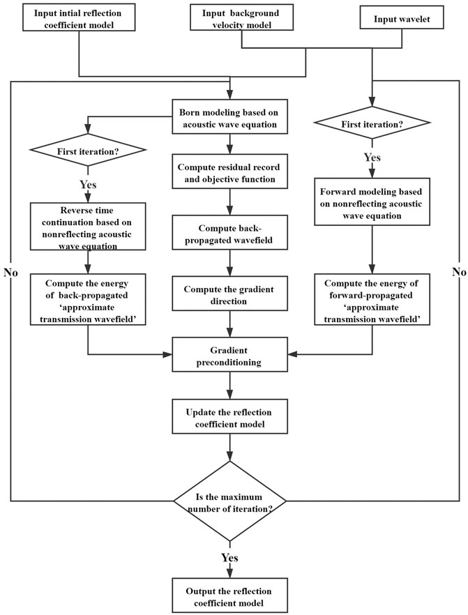
where g_t is the operator of GPTWE. The flowchart of the LSRTM using GPTWE is shown in Figure 1.

FIGURE 1

FIGURE 1. Flowchart of the LSRTM using GPTWE.

It should be noted that in the implementation process of the LSRTM using GPTWE, all the steps are the same as the LSRTM using GPSWE, except that the acoustic wave equation in calculating preconditioning operator is replaced with the non-reflecting acoustic wave equation, so the calculation of the LSRTM using GPTWE is essentially in agreement with the one using GPSWE. The LSRTM using GPSWE only needs to add one additional forward modeling and one additional reverse time continuation in the first iteration in comparison with the conventional LSRTM without gradient preconditioning. And the additional calculation is negligible compared with the LSRTM itself, which often needs hundreds of wavefield continuation. Therefore, theoretically, the computational efficiency of the three methods including the conventional LSRTM without gradient preconditioning, the LSRTM using GPSWE, and the LSRTM using GPTWE are basically equivalent.

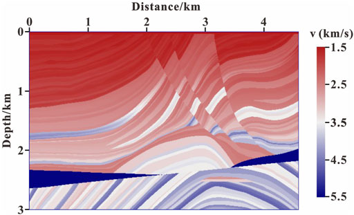
To test the suppressing effect of the non-reflecting acoustic wave equation on reflected waves, the forward modeling experiment was carried out based on the Marmousi model. The size of model is 4,600 m in length and 3,000 m in depth (as shown in Figure 2). The grid interval in the x and z directions is 8 m. A Ricker wavelet with a dominant frequency of 20 Hz is used as the source, which is excited at (2,300 m, 0 m). The accuracy in finite difference wavefield modeling is eighth order in space and second order in time. The time sampling step is 0.5 ms, and the maximum recording time is 3 s. The hybrid absorbing boundary condition (Xie et al., 2020) is used for boundary processing. Figure 3 illustrates the wavefront snapshots at 1.05 s simulated by the acoustic wave equation and the non-reflecting acoustic wave equation.

FIGURE 2

FIGURE 2. Marmousi velocity model.

FIGURE 3

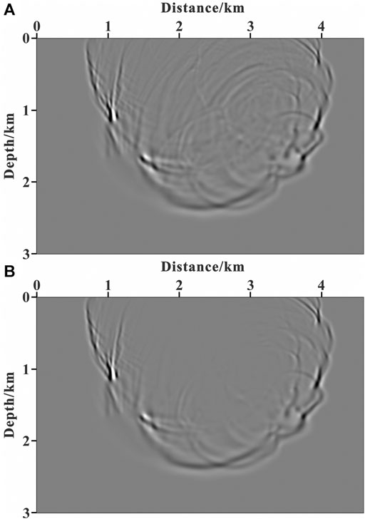
FIGURE 3. Wavefront snapshots of numeric modeling at 1.05 s: (A) based on the acoustic wave equation; (B) based on the non-reflecting acoustic wave equation.

From Figure 3, we can observe that the reflected waves in the wavefield simulated by the non-reflecting acoustic wave equation have been suppressed effectively, and the simulated wavefield is closer to a pure transmitted wavefield than that simulated by the acoustic wave equation. Therefore, in theory, it is more accurate to precondition the gradient using “approximate transmission wavefield” information simulated by the non-reflecting acoustic wave equation.

Marmousi Model Test

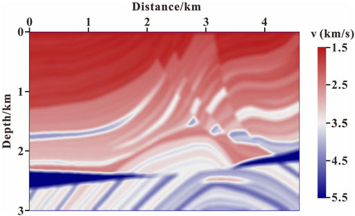
The Marmousi model in LSRTM Using the GPTWE is used to test the feasibility and accuracy of the algorithm in complex media conditions. The background velocity model used for LSRTM imaging is shown in Figure 4, which is the result of Gaussian smoothing of the original velocity model in Figure 2. A total of 116 shots are considered for imaging, and the shots are evenly distributed on the surface with the interval of 40 m. A total of 451 receivers are allotted for each shot, and the receivers are evenly distributed on both sides of each shot with 8-m interval. The observation data are generated by the full-waveform modeling (Eq. 1). The remaining experimental parameters are the same as those in LSRTM Using the GPTWE.

FIGURE 4

FIGURE 4. Background velocity model.

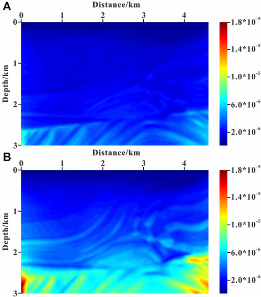
Figure 5 shows the preconditioners using GPSWE and GPTWE. In Figures 5A,B, we can observe that the preconditioning operator of GPTWE is more related to the model, and the deep illumination compensation is stronger. Figure 6 illustrates the imaging result of LSRTM after 60 iterations. Through the compassion between Figures 6A–C (marked by the dashed red circle), it can be seen that the imaging results of LSRTM based on gradient preconditioning are better than those without gradient preconditioning. Specifically, after 60 iterations, the LSRTM using GPTWE has the best amplitude preservation, the highest spatial resolution, and the highest imaging accuracy of deep part, followed by the LSRTM using GPSWE, and the LSRTM without gradient preconditioning has the worst imaging result.

FIGURE 5

FIGURE 5. Schematic description of the gradient preconditioning operator: (A) GPSWE; (B) GPTWE.

FIGURE 6

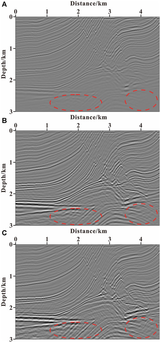
FIGURE 6. Imaging results of LSRTM after 60 iterations: (A) without gradient preconditioning; (B) using GPSWE; and (C) using GPTWE.

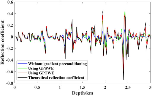
In order to compare the imaging effects of the previous three methods more clearly, we extract the imaging curves at x = 1960 m from the sections in Figure 6 and compare them with theoretical reflection coefficient curve, which is calculated using Eq. 3; Figure 7 is the single-trace display of imaging results after 60 iterations, where blue, green, red, and black are the single-trace curves of LSRTM without gradient preconditioning, using GPSWE, using GPTWE, and theoretical reflection coefficient, respectively. As observed from Figure 7, the imaging result of LSRTM using GPTWE is closest to the theoretical reflection coefficient curve, while the imaging result of LSRTM without gradient preconditioning is the different from the theoretical reflection coefficient curve at different imaging positions. Therefore, the amplitude preservation of the LSRTM using GPTWE is the highest, followed by the LSRTM using GPSWE, and the lowest without gradient preconditioning.

FIGURE 7

FIGURE 7. Single-trace display of imaging results after 60 iterations.

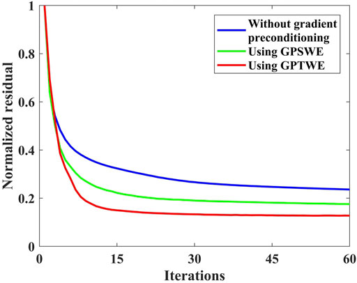
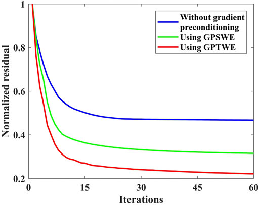
The convergence curves are shown in Figure 8 for this example, where blue, green, and red are the convergence curves of LSRTM without gradient preconditioning, using GPSWE, and using GPTWE, respectively. In Figure 8, it can be seen that the LSRTM using GPTWE has the fastest convergence rate and the smallest residual error, followed by the LSRTM using GPSWE, while the LSRTM without gradient preconditioning has the slowest convergence rate and converges to the largest value after 60 iterations.

FIGURE 8

FIGURE 8. Normalized residual curves.

Furthermore, the computational efficiency of the previous three methods is analyzed, as shown in Table 1. (The GPU used in this experiment is GeForce RTX 2080 Ti.) Table 1 shows that computational efficiency of those methods is basically the same. It is also consistent with the result of theoretical analysis in LSRTM Using the GPTWE.

TABLE 1

TABLE 1. Calculation time of LSRTM with 60 iterations.

Pluto Data Example

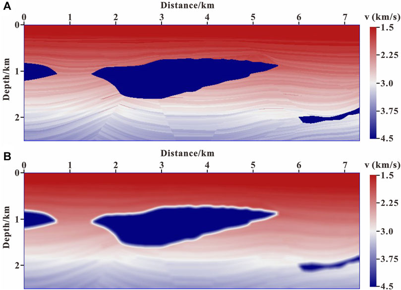
Due to the poor illumination beneath the salt bodies, the subsalt imaging problem has always been a challenging issue. So, in the second example, we performed LSRTM on the Pluto model to check the ability of LSRTM using GPTWE in recovering the weak events in the deep part and accelerating the convergence rate. Figure 9A shows the Pluto model, which is 7.33 km in length and 2.5 km in depth with a 10-m grid interval in the horizontal and vertical directions. And Figure 9B shows the smoothed background velocity model. The line involves 147 shots, and a total of 734 receivers are allotted for each shot. The observation data are generated by the full-waveform modeling (Eq. 1). The interval between shots is 50 m, and the interval between receivers is 10 m. The depth of shots and receivers are both 0 m. A Ricker wavelet with a 20 Hz dominant frequency is used to generate the data. The time sampling step is 1 ms, and the maximum recording time is 6 s. The accuracy in finite difference wavefield modeling is tenth order in space and second order in time. The hybrid absorbing boundary condition (Xie et al., 2020) is used for boundary processing.

FIGURE 9

FIGURE 9. Pluto velocity model: (A) real velocity model; (B) background velocity model.

The inverted images after 60 iterations with three different methods for the Pluto model are shown in Figure 10. As shown in Figure 10 (marked by the dashed red circle), the LSRTM without gradient preconditioning is difficult to image the structure below the salt bodies because of the poor illumination; the LSRTM using GPSWE is helpful for imaging the subsalt structures, but the event is weak and the horizontal balance is poor; the LSRTM using GPTWE can effectively improve the imaging accuracy of deep target, and the subsalt structures are clearer and more continuous than those of other images.

FIGURE 10

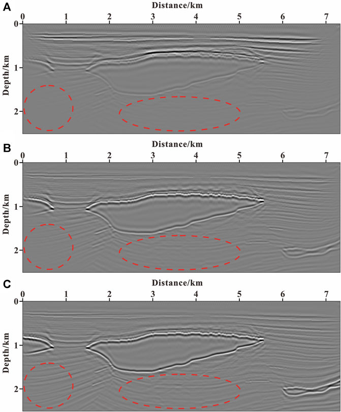
FIGURE 10. Imaging results of LSRTM after 60 iterations: (A) without gradient preconditioning; (B) using GPSWE; and (C) using GPTWE.

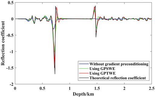
Analogously, the imaging curves and theoretical reflection coefficient curve at x = 3,500 m are displayed in Figure 11. As observed from Figure 11, the imaging result of LSRTM using GPTWE is closest to the theoretical reflection coefficient curve, especially in the deep part.

FIGURE 11

FIGURE 11. Single-trace display of imaging results after 60 iterations.

The convergence curves are plotted in Figure 12. It can be seen that after 60 iterations, the red curve for LSRTM using GPTWE has the fastest convergence rate and converges to the smallest value.

FIGURE 12

FIGURE 12. Normalized residual curves.

Conclusion and Prospect

Based on the calculation characteristics of LSRTM, this study proposes a gradient preconditioning approach using transmitted wave energy for LSRTM. In comparison with conventional methods, the imaging results of theoretical model tests show that the LSRTM using GPTWE can improve the imaging accuracy of deep target and speed up the convergence rate without significantly increasing the amount of calculation. In addition, this study only implements the two-dimensional LSRTM using GPTWE, and further extending the algorithm to three-dimensional migration will be the focus of subsequent research.

Data Availability Statement

The original contributions presented in the study are included in the article/Supplementary Material; further inquiries can be directed to the corresponding author.

Author Contributions

CX contributed to writing—original draft. PS helped with conceptualization and project administration. XL assisted with formal analysis. JT helped with software. SW framed the methodology. BZ provided suggestions.

Funding

This research is jointly funded by the National Natural Science Foundation of China (No. 42074138), Fundamental Research Funds for the Central Universities (201964016), and the Major Scientific and Technological Innovation Project of Shandong Province (2019JZZY010803).

Conflict of Interest

The authors declare that the research was conducted in the absence of any commercial or financial relationships that could be construed as a potential conflict of interest.

Publisher’s Note

All claims expressed in this article are solely those of the authors and do not necessarily represent those of their affiliated organizations, or those of the publisher, the editors, and the reviewers. Any product that may be evaluated in this article, or claim that may be made by its manufacturer, is not guaranteed or endorsed by the publisher.

References

Baysal, E., Kosloff, D. D., and Sherwood, J. W. C. (1984). A Two‐way Nonreflecting Wave Equation. Geophysics 49, 132–141. doi:10.1190/1.1441644

CrossRef Full Text | Google Scholar

Baysal, E., Kosloff, D. D., and Sherwood, J. W. C. (1983). Reverse Time Migration. Geophysics 48, 1514–1524. doi:10.1190/1.1441434

CrossRef Full Text | Google Scholar

Choi, Y., Min, D.-J., and Shin, C. (2008). Frequency-domain Elastic Full Waveform Inversion Using the New Pseudo-hessian Matrix: Experience of Elastic Marmousi-2 Synthetic Data. Bull. Seismological Soc. America 98 (5), 2402–2415. doi:10.1785/0120070179

CrossRef Full Text | Google Scholar

Claerbout, J. F. (1992). Earth Soundings Analysis: Processing versus Inversion. Blackwell Scientific Publications.

Google Scholar

Dai, W., Boonyasiriwat, C., and Schuster, G. T. (2010). 3D Multi-Source Least-Squares Reverse Time Migration. 80th Annu. Int. Meet. SEG. Denver, 3120–3124. doi:10.1190/1.3513494

CrossRef Full Text | Google Scholar

Dai, W., Fowler, P., and Schuster, G. T. (2012). Multi-source Least-Squares Reverse Time Migration. Geophys. Prospecting 60, 681–695. doi:10.1111/j.1365-2478.2012.01092.x

CrossRef Full Text | Google Scholar

Dai, W., and Schuster, G. T. (2013). Plane-wave Least-Squares Reverse-Time Migration. Geophysics 78, S165–S177. doi:10.1190/GEO2012-0377.1

CrossRef Full Text | Google Scholar

Fang, J., Zhou, H., Chen, H., Wang, N., Wang, Y., Sun, P., et al. (2019). Source-independent Elastic Least-Squares Reverse Time Migration. Geophysics 84, S1–S16. doi:10.1190/GEO2017-0847.1

CrossRef Full Text | Google Scholar

Fletcher, R. P., Du, X., and Fowler, P. J. (2009). Reverse Time Migration in Tilted Transversely Isotropic (TTI) media. Geophysics 74, WCA179–WCA187. doi:10.1190/1.3269902

CrossRef Full Text | Google Scholar

Gao, K., Chi, B. X., and Huang, L. J. (2017). “Elastic Least-Squares Reverse-Time Migration with Implicit Wavefield Separation,” in 87th Annual International Meeting, September 23, 2017 to September 29, 2017 (Houston: SEG), 4389–4394.

CrossRef Full Text | Google Scholar

Gao, W., Matharu, G., and Sacchi, M. D. (2020). Fast Least-Squares Reverse Time Migration via a Superposition of Kronecker Products. Geophysics 85, S115–S134. doi:10.1190/GEO2019-0254.1

CrossRef Full Text | Google Scholar

Gerhard Pratt, R. G., Shin, C., and Hicks, G. J. (1998). Gauss-Newton and Full Newton Methods in Frequency-Space Seismic Waveform Inversion. Geophys. J. Int. 133, 341–362. doi:10.1046/j.1365-246x.1998.00498.x

CrossRef Full Text | Google Scholar

Gong, X. B., Wang, S. C., and Han, L. G. (2019). Sparse Least-Squares Reverse Time Migration of Small Scatters in Seismic Exploration. Chin. J. Geophys. 62, 4028–4038. doi:10.6038/cjg2019M0420

CrossRef Full Text | Google Scholar

Gu, B., Li, Z., Yang, P., Xu, W., and Han, J. (2017). Elastic Least-Squares Reverse Time Migration with Hybrid L1/l2 Misfit Function. Geophysics 82, S271–S291. doi:10.1190/GEO2016-0235.1

CrossRef Full Text | Google Scholar

Guo, P., and McMechan, G. A. (2018). Compensating Q Effects in Viscoelastic media by Adjoint-Based Least-Squares Reverse Time Migration. Geophysics 83, S151–S172. doi:10.1190/GEO2017-0235.1

CrossRef Full Text | Google Scholar

Guo, Z. B., and Li, Z. C. (2014). True-amplitude Imaging Based on Least-Squares Reverse Time Migration. Oil Geophys. Prospecting 49, 113–120. doi:10.13810/j.cnki.issn.1000-7210.2014.01.014

CrossRef Full Text | Google Scholar

Hu, J., Wang, H., Fang, Z., Li, T., and Zhang, J. (2016). Efficient Amplitude Encoding Least-Squares Reverse Time Migration Using Cosine Basis. Geophys. Prospecting 64, 1483–1497. doi:10.1111/1365-2478.12356

CrossRef Full Text | Google Scholar

Huang, J. P., Cao, X. L., Li, Z. C., Sun, Y. S., Li, C., and Gao, G. C. (2014). Least Square Reverse Time Migration in High Resolution Imaging of Near Surface. Oil Geophys. Prospecting 49, 107–112. doi:10.13810/j.cnki.issn.1000-7210.2014.01.013

CrossRef Full Text | Google Scholar

Huang, J. P., Li, C., Li, Q. Y., Guo, S. J., Duan, X. B., Li, J. G., et al. (2015). Least-squares Reverse Time Migration with Static Plane-Wave Encoding. Chin. J. Geophys. 58, 2046–2056. doi:10.6038/cjg20150619

CrossRef Full Text | Google Scholar

Li, C., Huang, J., Li, Z., and Wang, R. (2018). Plane-wave Least-Squares Reverse Time Migration with a Preconditioned Stochastic Conjugate Gradient Method. Geophysics 83, S33–S46. doi:10.1190/GEO2017-0339.1

CrossRef Full Text | Google Scholar

Li, F., Gao, J., Gao, Z., Jiang, X., and Sun, W. (2020). Least-squares Reverse Time Migration with Sparse Regularization in the 2D Wavelet Domain. Geophysics 85, S313–S325. doi:10.1190/GEO2018-0763.1

CrossRef Full Text | Google Scholar

Liu, F., Zhang, G., Morton, S. A., and Leveille, J. P. (2011). An Effective Imaging Condition for Reverse-Time Migration Using Wavefield Decomposition. Geophysics 76, S29–S39. doi:10.1190/1.3533914

CrossRef Full Text | Google Scholar

Liu, X., and Liu, Y. (2019). Deghosting-based Reverse Time Migration with Free-Surface Multiples. Geophys. J. Int. 216, 1191–1200. doi:10.1093/gji/ggy486

CrossRef Full Text | Google Scholar

Liu, X., Liu, Y., Huang, X., and Li, P. (2016). Least-squares Reverse-Time Migration with Cost-Effective Computation and Memory Storage. J. Appl. Geophys. 129, 200–208. doi:10.1016/j.jappgeo.2016.03.009

CrossRef Full Text | Google Scholar

McMechan, G. A. (1983). Migration by Extrapolation of Time-dependent Boundary Values*. Geophys. Prospect 31, 413–420. doi:10.1111/j.1365-2478.1983.tb01060.x

CrossRef Full Text | Google Scholar

Nemeth, T., Wu, C., and Schuster, G. T. (1999). Least‐squares Migration of Incomplete Reflection Data. Geophysics 64, 208–221. doi:10.1190/1.144455710.1190/1.1444517

CrossRef Full Text | Google Scholar

Plessix, R.-E. (2006). A Review of the Adjoint-State Method for Computing the Gradient of a Functional with Geophysical Applications. Geophys. J. Int. 167, 495–503. doi:10.1111/j.1365-246X.2006.02978.x

CrossRef Full Text | Google Scholar

Qu, Y. M., Li, J. L., Wang, Y. C., Li, Z. C., Sun, W. Z., and Sun, J. Z. (2019). Correction of Viscoelasticity and Anisotropy in Least-Squares Reverse Time Migration: a Bohai Bay Seismic Case Study. Chin. J. Geophys. 62, 2203–2216. doi:10.6038/cjg2019M0597

CrossRef Full Text | Google Scholar

Ren, Z., Liu, Y., and Sen, M. K. (2017). Least-squares Reverse Time Migration in Elastic media. Geophys. J. Int. 208, 1103–1125. doi:10.1093/gji/ggw443

CrossRef Full Text | Google Scholar

Rocha, D., and Sava, P. (2018). Elastic Least-Squares Reverse Time Migration Using the Energy Norm. Geophysics 83, S237–S248. doi:10.1190/GEO2017-0465.1

CrossRef Full Text | Google Scholar

Shin, C., Jang, S., and Min, D.-J. (2001). Improved Amplitude Preservation for Prestack Depth Migration by Inverse Scattering Theory. Geophys. prospecting 49 (5), 592–606. doi:10.1046/j.1365-2478.2001.00279.x

CrossRef Full Text | Google Scholar

Song, P., Tan, J., Liu, Z., Zhang, X., Liu, B., Yu, K., et al. (2019). Time-domain Full Waveform Inversion Using the Gradient Preconditioning Based on Transmitted Wave Energy. J. Ocean Univ. China 18, 859–867. doi:10.1007/s11802-019-3783-z

CrossRef Full Text | Google Scholar

Sun, J., Fomel, S., and Ying, L. (2016). Low-rank One-step Wave Extrapolation for Reverse Time Migration. Geophysics 81, S39–S54. doi:10.1190/GEO2015-0183.1

CrossRef Full Text | Google Scholar

Symes, W. W. (2007). Reverse Time Migration with Optimal Checkpointing. Geophysics 72, SM213–SM221. doi:10.1190/1.2742686

CrossRef Full Text | Google Scholar

Tan, S., and Huang, L. (2014). Least-squares Reverse-Time Migration with a Wavefield-Separation Imaging Condition and Updated Source Wavefields. Geophysics 79, S195–S205. doi:10.1190/GEO2014-0020.1

CrossRef Full Text | Google Scholar

Wong, M., Biondi, B. L., and Ronen, S. (2015). Imaging with Primaries and Free-Surface Multiples by Joint Least-Squares Reverse Time Migration. Geophysics 80, S223–S235. doi:10.1190/GEO2015-0093.1

CrossRef Full Text | Google Scholar

Wu, D., Yao, G., Cao, J., and Wang, Y. (2016). Least-squares RTM with L1 Norm Regularisation. J. Geophys. Eng. 13, 666–673. doi:10.1088/1742-2132/13/5/666

CrossRef Full Text | Google Scholar

Xie, C., Song, P., Tan, J., Liu, B., Li, J., Yu, K., et al. (2020). Cosine-type Weighted Hybrid Absorbing Boundary Based on the Second-Order Higdon Boundary Condition and its GPU Implementation. J. Geophys. Eng. 17, 231–248. doi:10.1093/jge/gxz102

CrossRef Full Text | Google Scholar

Yang, J., Li, Y. E., Liu, Y., and Zong, J. (2020). Least-squares Extended Reverse Time Migration with Randomly Sampled Space Shifts. Geophysics 85, S357–S369. doi:10.1190/GEO2019-0536.1

CrossRef Full Text | Google Scholar

Yang, J., Liu, Y., Li, Y. E., Cheng, A., Dong, L., and Du, Y. (2019). Joint Least-Squares Reverse Time Migration of Primary and Prismatic Waves. Geophysics 84, S29–S40. doi:10.1190/GEO2017-0850.1

CrossRef Full Text | Google Scholar

Yang, J., and Zhu, H. (2019). Viscoacoustic Least-Squares Reverse Time Migration Using a Time-Domain Complex-Valued Wave Equation. Geophysics 84, S479–S499. doi:10.1190/GEO2018-0804.1

CrossRef Full Text | Google Scholar

Yao, G., and Jakubowicz, H. (2016). Least-squares Reverse-Time Migration in a Matrix-Based Formulation. Geophys. Prospecting 64, 611–621. doi:10.1111/1365-2478.12305

CrossRef Full Text | Google Scholar

Yoon, K., and Marfurt, K. J. (2006). Reverse-time Migration Using the Poynting Vector. Exploration Geophys. 37, 102–107. doi:10.1071/EG06102

CrossRef Full Text | Google Scholar

Zhang, Q., Zhou, H., Chen, H., and Wang, J. (2016). Least-squares Reverse Time Migration with and without Source Wavelet Estimation. J. Appl. Geophys. 134, 1–10. doi:10.1016/j.jappgeo.2016.08.003

CrossRef Full Text | Google Scholar

Zhang, Y., Duan, L., and Xie, Y. (2015). A Stable and Practical Implementation of Least-Squares Reverse Time Migration. Geophysics 80, V23–V31. doi:10.1190/GEO2013-0461.1

CrossRef Full Text | Google Scholar

Zhang, Z., Huang, L., and Lin, Y. (2012). “A Wave-Energy-Based Precondition Approach to Full-Waveform Inversion in the Time Domain,” in 82nd Annual International Meeting, November 4 to November 9, 2012 (Las Vegas: SEG), 1–5. doi:10.1190/segam2012-1555.1

CrossRef Full Text | Google Scholar

Zhao, Z., and Sen, M. K. (2018). Fast Image-Domain Target-Oriented Least-Squares Reverse Time Migration. Geophysics 83, A81–A86. doi:10.1190/GEO2018-0033.1

CrossRef Full Text | Google Scholar